Change-plane analysis for subgroup detection with a continuous treatment

Summary:

Detecting and characterizing subgroups with differential effects of a binary treatment has been widely studied and led to improvements in patient outcomes and population risk management. Under the setting of a continuous treatment, however, such investigations remain scarce. We propose a semiparametric change-plane model and consequently a doubly robust test statistic for assessing the existence of two subgroups with differential treatment effects under a continuous treatment. The proposed testing procedure is valid when either the baseline function for the covariate effects or the generalized propensity score function for the continuous treatment is correctly specified. The asymptotic distributions of the test statistic under the null and local alternative hypotheses are established. When the null hypothesis of no subgroup is rejected, the change-plane parameters that define the subgroups can be estimated. This paper provides a unified framework of the change-plane method to handle various types of outcomes, including the exponential family of distributions and time-to-event outcomes. Additional extensions with nonparametric estimation approaches are also provided. We evaluate the performance of our proposed methods through extensive simulation studies under various scenarios. An application to the Health Effects of Arsenic Longitudinal Study with a continuous environmental exposure of arsenic is presented.

1. Introduction

Subgroup identification has become an increasingly important topic in many research areas including precision medicine and environmental health. Because of patients’ heterogeneity, it is well recognized that treatment effects in a randomized trial can vary across the study population (Imai and Ratkovic, 2013; Kent et al., 2018). The traditional one-size-fits-all strategy may not benefit everyone in reality. The health risk of environmental hazards or occupational exposures is never wholly uniform in population. People respond differently to an exposure due to heterogeneity in genetics, individual characteristics, lifestyles, and socioeconomic status (Hirvonen, 1995; Kosnik et al., 2021). Consequently, identifying meaningful subgroups with differential treatment or exposure effects can lead to informed clinical decisions, identification of susceptible population, improved efficiency of risk assessment, and health policymaking.

Assuming that subgroups do exist, several data-driven methods have been proposed for subgroup characterization and estimating differential treatment effects under the setting of a binary treatment. Examples include proposing a selection impact curve for treatment selection (Song and Pepe, 2004), moving average procedure (Bonetti and Gelber, 2004), “Virtual Twins” method (Foster et al., 2011), and parametric scoring system approaches (Cai et al., 2011; Zhao et al., 2013). Other developments of data-driven approaches for subgroup analysis in clinical trials are well summarized in the tutorial by Lipkovich et al. (2017). Recently, several methods have been developed for subgroup characterization using change-plane models. Wei and Kosorok (2018) introduced a non-regular Cox model with a change-plane in covariate space that divides the population into two subgroups. Aiming to identify possible multiple (more than two) subgroups, Li et al. (2021) proposed a multi-threshold change-plane regression model with a novel two-step approach to determine the number of subgroups, location of thresholds, and regression parameters. There are other developments for subgroup identification based on the idea of change-point detection, including Wang et al. (2019) and Li et al. (2019), among others.

Before researchers proceed to estimate differential effects for different subgroups, an important statistical concern is regarding the existence of meaningful subgroups (Assmann et al., 2000; Wang et al., 2007). Any aggressive use of subgroup analysis without performing a valid statistical hypothesis testing procedure may lead to false positive findings, where subgroups are observed by chance. If post-hoc statistical tests are conducted over many possible subgroups, power loss is another issue after adjusting for multiple testing. Under the setting of binary treatment, Shen and He (2015) adapted a logistic-normal mixture model and proposed a likelihood-based test to check the existence of a subgroup with an enhanced treatment effect. Wu et al. (2016) extended to a logistic-Cox mixture model when the outcome of interest was time-to-event with right censoring. Both methods require strong parametric assumptions for covariate effects. Utilizing the change-plane technique, Fan et al. (2017) adapted a semiparametric model and proposed a double-robust test statistic for subgroup detection and sample size calculation. Subsequently, Kang et al. (2017) extended the double-robust test to survival data by assuming a change-plane proportional hazards model under mild assumptions for censoring. Recently, Huang et al. (2020) developed a subgroup testing procedure based on maximum likelihood ratio statistics for binary outcome and further incorporated an inverse probability weighting technique to allow for unbiased testing under a two-phase sampling design.

In practice, the treatment or exposure of interest can be continuous. For example, proper dosing of warfarin is vital to prevent thrombosis, as overdosing may predispose patients to high risk of bleeding and underdosing may diminish the drug’s effect. With environmental exposures, increasing levels of air pollutants PM and NO₂ are associated with adverse health risks, such as lung cancer or cardiovascular diseases (Costa et al., 2014). A motivating study for this manuscript investigated the effect of continuous arsenic exposure on blood pressure in Bangladesh adolescents (Chen et al., 2019), and found that increasing level of arsenic exposure from drinking water was associated with elevated blood pressure in adolescence. In particular, the association was stronger within a subgroup of adolescents with high body mass index (BMI). Although several methods have been developed under the topic of optimal individual treatment regime (ITR) focusing on continuous treatment (Chen et al., 2016; Park et al., 2021), statistical methods for subgroup identification under a continuous treatment setting are scarce, especially for testing the existence of subgroups with differential effects. There is a fundamental difference in the goals for identifying optimal ITR versus detecting subgroups: the former aims to identify a specific level of treatment that maximizes the beneficial clinical outcome for patients given individual characteristics, while the latter is to test the existence of a group of subjects among the study population with differential effects. Our work here focuses on the latter.

In this article, we consider a semiparametric change-plane model for testing the existence of a subgroup with differential treatment effects when the treatment is continuous. The “treatment” is a general term here and can refer to either controlled continuous intervention dosage in clinical trials or continuous exposures or risk factors in observational studies. The flexible change-plane model consists of an unknown baseline effect component and an interaction component between an unknown differential treatment function and a subgroup indicator that is explicitly defined by a change-plane in the covariate space. Testing the null hypothesis of homogeneous treatment function at every possible value of the continuous treatment is nontrivial. We propose a double-robust test statistic for testing the existence of a subgroup with differential treatment effects. Here the double robustness property ensures that the proposed test is valid under the null hypothesis when either the baseline effect function or the generalized propensity score (GPS) function for the continuous treatment (Imai and van Dyk, 2004; Hirano and Imbens, 2004) is correctly specified. When the null hypothesis is rejected, the change-plane parameters that define the subgroup can be estimated by maximizing the test statistic. Furthermore, we complete the proposed change-plane modeling framework by providing extensions to handle outcomes from general exponential family distributions and censored survival data. In addition to the parametric modeling approach that utilizes double robustness property, we also explore nonparametric estimation alternatives for baseline effect function and GPS function, which provide modeling flexibility and protection against model misspecification. A practical contribution also includes R codes available online to implement the proposed procedure.

The rest of this paper is organized as follows. In Section 2, we introduce the semiparametric change-plane model and the proposed test statistic for continuous outcome. The asymptotic distributions of the proposed test statistic under both the null and local alternative hypotheses are established. The nonparametric estimation approaches are discussed. Section 3 provides extensions to handle other types of outcomes. Section 4 presents extensive numerical studies to evaluate the performance of the proposed test. In Section 5, we demonstrate the proposed test for subgroup identification using the study on arsenic and adolescent blood pressure from the Health Effects of Arsenic Longitudinal Study (HEALS). Remarks are discussed in Section 6. All technical proofs and additional simulation results are provided in Web Appendix at Biometrics online.

2. Method

2.1. Change-plane model for continuous outcome and proposed test statistic

Consider a randomized trial or observational study with n independent subjects. For the ith subject, let X_i denote a vector of baseline covariates including an intercept term of 1, Y_i denote a continuous response of interest, and A_i be the treatment that is continuous over a bounded interval 𝒜. Without loss of generality, we assume 𝒜 = [−1, 1]. The observed data consist of n independent and identically distributed observations $\left\{{\left(X_i^T,A_i,Y_i\right)}^T,i=1,\dots ,n\right\}$.

We consider the following semiparametric change-plane model for a continuous outcome,

$$Y_i=\mu \left(X_i\right)+\psi \left(A_i\right)I\left({\theta }^T{X}_i⩾0\right)+{ϵ}_i,$$ (1)

where μ(X_i) is an unknown baseline covariate mean function, I(θ^T X_i ⩾ 0) is a change plane defining the subgroup with an unknown differential treatment effect ψ(A_i), θ = (θ₀, …,θ_p)^T denotes the corresponding change-plane parameters, and E(ϵ_i|A_i, X_i) = 0. For identifiability, we assume that ∥θ∥ = 1 and ψ(0) = 0.

Our interest is to test the existence of a subgroup with differential treatment effects, which, under model (1), corresponds to testing H₀ : ψ(a) = 0, ∀a ∈ 𝒜 vs. H_a : ψ(a) ≠ 0 for a subset of 𝒜 with positive probability. We assume ψ(a) is a continuous function and can be well approximated by ψ(a) = τ^T B(a), where B(a) are q spline basis functions (e.g., B-spline), and q depends on the specified number of knots and degrees of the spline functions. Consequently, the null hypothesis H₀ : ψ(a) = 0 for all a ∈ 𝒜 translates to H₀ : τ = 0. Note that the change-plane parameters θ disappear from the model under H₀, which makes the testing nonstandard. The null model remains the same under different spline approximations, and thus the proposed test with spline approximations would maintain a proper type I error but may lose power under alternatives when ψ(a) is not well approximated by the specified finite spline representations.

Given fixed θ, the change-plane model (1) belongs to the class of semiparametric models considered in Robins and Rotnitzky (2001). We consider the following double-robust estimating equations for τ based on the semiparametric theory (Tsiatis, 2006),

$$\sum _{i=1}^{n}I\left({\theta }^T{X}_i⩾0\right)\left\{B\left(A_i\right)-m\left(X_i\right)\right\}\left\{Y_i-\mu \left(X_i\right)-{\tau }^{T}B\left(A_i\right)I\left({\theta }^T{X}_i⩾0\right)\right\}=0,$$ (2)

where $m\left(X_i\right)={\left(m_1\left(X_i\right),\dots ,m_q\left(X_i\right)\right)}^T,m_l\left(X_i\right)={\int }_{a\in 𝒜}{B}_l(a)\pi \left(a\mid X_i\right)da$ is the conditional expectation of B_l(A), l = 1, …,q, with respect to the continuous treatment A, and π(a|X_i) is the GPS function characterizing the conditional distribution of A. The double robustness property of (2) ensures that the proposed score function is valid under the null hypothesis when either the model for the baseline covariate mean function μ(X) or the GPS function is correctly specified, and thus facilitates the use of parametric modeling of baseline function or the GPS function. We adopt parametric models μ(X; β) (e.g. linear regression) and π(A|X; γ) (e.g. truncated normal distribution) for their counterparts, where β and γ are vectors of coefficients characterizing the effects of X on outcome Y and on treatment A, respectively. We conduct a two-step procedure and first estimate β and γ under the null hypothesis. Under the specified models, $\widehat{\eta }={\left({\widehat{\beta }}^T,{\widehat{\gamma }}^T\right)}^T$ denotes the estimates from the following score equations,

$$\sum _{i=1}^n{S}_2\left(X_i,Y_i;\beta \right)=\sum _{i=1}^n\left\{\partial \mu \left(X_i;\beta \right)/\partial \beta \right\}\left\{Y_i-\mu \left(X_i;\beta \right)\right\}=0,$$

$$\sum _{i=1}^n{S}_3\left(X_i,A_i;\gamma \right)=\sum _{i=1}^n\partial \text{log}\text{L}\left(\gamma ;X_i,A_i\right)/\partial \mathit{\gamma }=0,$$

where L(γ; X, A) denotes the likelihood function corresponding to the parametric GPS specification. Given $\widehat{\eta }$, score function (2) under the null hypothesis becomes

$$\sum _{i=1}^n{S}_1\left(X_i,Y_i,A_i,\widehat{\eta };\theta \right)=\sum _{i=1}^{n}I\left({\theta }^T{X}_i⩾0\right)\left\{B\left(A_i\right)-m\left(X_i;\widehat{\gamma }\right)\right\}\left\{Y_i-\mu \left(X_i;\widehat{\beta }\right)\right\}.$$ (3)

When the distribution of continuous treatment is known, such as under a randomized trial, the proposed test is always robust against any misspecification of posited parametric model μ(X; β). The parametric modeling approach has advantages of easy implementation, especially with large samples, but model misspecification could affect the proposed test’s power. In Section 2.3, we discuss nonparametric estimation alternatives to offer additional flexibility, especially under the setting of observational study where both the baseline covariate mean function and the GPS function are to be estimated.

Since the change-plane parameters θ in model (1) are only present under H_a, it makes the testing problem nonregular and the standard asymptotic framework for hypothesis testing no longer applicable (Davies, 1987; Andrews, 2001; Fan et al., 2017). Therefore, we consider a supremum of normalized squared test statistics:

$$T_n=\underset{\theta \in \Theta }{\text{sup}}{\left\{\sum _{i=1}^n{S}_1\left(X_i,Y_i,A_i,\widehat{\eta };\theta \right)\right\}}^T\left\{n{\widehat{V}}_n{(\theta )}^{-1}\right\}\left\{\sum _{i=1}^n{S}_1\left(X_i,Y_i,A_i,\widehat{\eta };\theta \right)\right\},$$ (4)

where Θ = {θ ∈ R^p+1 : ∥θ∥ = 1} and ${\widehat{V}}_n(\theta )$ is a consistent estimator for the variance of $n^{-1/2}{\sum }_{i=1}^n{S}_1\left(X_i,Y_i,A_i,\widehat{\eta };\theta \right)$ under H₀, the specification of which will be given in Section 2.2. Due to the difficulty of obtaining the supremum over the entire space Θ, we calculate the maximum using the numerical approximation of the supremum by taking a dense grid of points on the surface of a unit ball of p + 1 dimensions. We employ a sphere coordinates transformation Γ = (Γ₁, …, Γ_p)^T → θ that automatically satisfies the unit ball constraint, where Γ_p ranges over [0, 2π) and the rest elements in Γ range over [0, π]. Specifically, the transformation is as follows,

$${\theta }_0=\text{cos}\left({\Gamma }_1\right),{\theta }_1=\text{sin}\left({\Gamma }_1\right)\text{cos}\left({\Gamma }_2\right),\dots ,{\theta }_p=\text{sin}\left({\Gamma }_1\right)\text{sin}\left({\Gamma }_2\right)\dots \text{sin}\left({\Gamma }_p\right).$$

We then evaluate the proposed test statistic over a set of grid points of Γ over [0, π]^p−1×[0, 2π) and choose the maximum value to approximate T_n.

2.2. Asymptotic distribution of test statistic T_n

We establish the asymptotic distributions of T_n under the null and local alternative hypotheses.

Theorem 1: Assume either the baseline mean function or the GPS function is correctly specified. Under the null hypothesis and regularity conditions stated in Appendix, T_n converges in distribution to sup_θ∈ΘG(θ)^T G(θ) as n → ∞, where G(θ) is a mean-zero multivariate Gaussian process with the asymptotic covariance function

$$\Sigma \left({\theta }_1,{\theta }_2\right)={\left\{\mathit{\text{diag}}\left(K_{{\theta }_1,{\theta }_2}\right)\right\}}^{-1/2}{K}_{{\theta }_1,{\theta }_2}{\left\{\mathit{\text{diag}}\left(K_{{\theta }_1,{\theta }_2}\right)\right\}}^{-1/2}$$

for any θ₁, θ₂ ∈ Θ. Here, $K_{{\theta }_1,{\theta }_2}=E[S_{1\ast }\left(X,Y,A,{\eta }_0;{\theta }_1\right){\mathit{S}}_{1\ast }{(X,Y,A,{\eta }_0;{\theta }_2)}^T]$ is the true value of η. The definition of S_1∗(X, Y, A, η₀; θ) is provided in Web Appendix.

Theorem 2: Assume either the baseline mean function or the GPS function is correctly specified. Under the local alternative hypothesis, $H_{an}:\tau =\zeta /\sqrt{n}$ for non-zero ζ, and regularity conditions stated in Appendix, T_n converges in distribution to sup_θ∈ΘG(θ; ζ)^T G(θ; ζ) as n → ∞, where G(θ; ζ) is a multivariate Gaussian process with the mean function W(θ) and covariance function Σ(θ₁, θ₂). Let m₀(X) be the expectation of splines given the true GPS model. The mean function is

$$W(\theta )=E\left[\sum _{i=1}^{n}I\left({\theta }^{T}X⩾0,{\theta }_0^{T}X⩾0\right)\left\{m_0(X)-m\left(X;{\gamma }_0\right)\right\}{\zeta }^T{m}_0(X)\right]{\left\{\mathit{\text{diag}}\left(K_{\theta ,\theta }\right)\right\}}^{-1/2},$$

where K_{θ, θ} = E[S_1∗(X, Y, A, η₀; θ)S_1∗(X, Y, A, η₀; θ)^T] is positive semi-definite.

To obtain the critical values for the proposed test, we suggest a resampling method to numerically approximate the limiting null distribution of the test statistic. Define the estimate of S_1∗(X, Y, A, η₀; θ) as

$${\widehat{S}}_{1\ast }(X,Y,A,\widehat{\eta };\theta )=S_1(X,Y,A,\widehat{\eta };\theta )-{\widehat{D}}_1^T{\widehat{C}}_1^{-1}{S}_2(X,Y;\widehat{\beta })-{\widehat{D}}_2^T{\widehat{C}}_2^{-1}{S}_3(X,A;\widehat{\mathit{\gamma }}),$$

where, ${\widehat{D}}_1=n^{-1}{\sum }_{i=1}^n\partial S_1\left(X_i,Y_i,A_i,\eta ;\theta \right)/{\partial \beta |}_{\eta =\widehat{\eta }}$, ${\widehat{D}}_2=n^{-1}{\sum }_{i=1}^n\partial S_1\left(X_i,Y_i,A_i,\eta ;\theta \right)/{\partial \mathit{\gamma }|}_{\eta =\widehat{\eta }}$, ${\widehat{C}}_1=n^{-1}{\sum }_{i=1}^n\partial S_2\left(X_i,Y_i;\beta \right)/{\partial {\beta }^T|}_{\beta =\widehat{\beta }}$, ${\widehat{C}}_2=n^{-1}{\sum }_{i=1}^n\partial S_3\left(X_i,A_i;\mathit{\gamma }\right)/{\partial {\mathit{\gamma }}^T|}_{\mathit{\gamma }=\widehat{\mathit{\gamma }}}$ are the empirical estimates of their theoretical counterparts, and the variance estimator ${\widehat{V}}_n(\theta )=n^{-1}{\sum }_{i=1}^n\left\{{\widehat{S}}_{1\ast }\left(X_i,Y_i,A_i,\widehat{\eta };\theta \right)\right\}{\left\{{\widehat{S}}_{1\ast }\left(X_i,Y_i,A_i,\widehat{\eta };\theta \right)\right\}}^T$. The perturbed test statistic is

$$T_n^{\ast }=\underset{\theta \in \Theta }{\text{sup}}{\left\{\sum _{i=1}^n{\xi }_i{\widehat{S}}_{1\ast }\left(X_i,Y_i,A_i,\widehat{\eta };\theta \right)\right\}}^T\left\{n{\widehat{V}}_n{(\theta )}^{-1}\right\}\left\{\sum _{i=1}^n{\xi }_i{\widehat{S}}_{1\ast }\left(X_i,Y_i,A_i,\widehat{\eta };\theta \right)\right\},$$ (5)

where ξ₁, …,ξ_n are i.i.d. standard normal random variables independent of the data. Conditioning on the observed data, $T_n^{\ast }$ has the same asymptotic distribution as T_n under the null hypothesis. The empirical distribution of $T_n^{\ast }$ can be obtained by repeatedly generating a large number of perturbed test statistics, and the critical value C_1−α is computed as the upper α-th quantile of the empirical distribution of $T_n^{\ast }$. When T_n > C_1−α, we reject the null hypothesis at the α level and can estimate the change-plane parameters by

$$\widehat{\theta }=\underset{\theta \in \Theta }{\text{arg}\text{sup}}{\left\{\sum _{i=1}^n{\widehat{S}}_1\left(X_i,Y_i,A_i,\widehat{\eta };\theta \right)\right\}}^T\left\{n{\widehat{V}}_n{(\theta )}^{-1}\right\}\left\{\sum _{i=1}^n{\widehat{S}}_1\left(X_i,Y_i,A_i,\widehat{\eta };\theta \right)\right\}.$$ (6)

Thus, the identified subgroup is $\left\{i:{\widehat{\theta }}^T{X}_i⩾0\right\}$.

In our simulation studies, we notice that the stability of the finite-sample variance matrix estimate ${\widehat{V}}_n(\theta )$ at the margin of space Θ may impact the numerical performance. When the size of a subgroup is extremely small or large at a fixed θ, the inverse of the estimated variance matrix could be numerically unstable. Therefore, we constrain the searching within the space of Θ such that the size of a potential subgroup is limited to be within the range 10%−90% of the total sample size for the purpose of numerical stability. Specifically, when searching over the unit ball for the change-plane parameters θ, any potential θ that generate a subgroup smaller than 10% of the total sample population is omitted. Applying this restriction should not conflict with our interest of identifying a subgroup with differential treatment effects with a reasonable subgroup size.

2.3. Nonparametric estimation approach

The double-robust property discussed above ensures the validity of our proposed test under H₀ when either the baseline covariate mean function or the GPS function is correctly specified. This may be challenging when multiple covariates exist with possible nonlinear or interaction effects. Indeed, we can also adopt nonparametric estimation approaches for π(X) and μ(X), such as random forest or neural network.

In addition to offering more flexibility and avoiding model misspecification, nonparametric estimation approaches can lead to a simpler derivation of the asymptotic variance for the test statistic. Given that the GPS function π(X) and baseline covariate mean function μ(X) both are estimated at proper convergence rates (Farrell et al., 2021), the remaining terms are at smaller order and thus can be ignored in the calculation of the asymptotic variance for the test statistic. On the downside, tuning parameter selection and large sample size are needed for nonparametric estimation approaches and may impact the performance in a finite sample. In our simulations, we observe small power loss by using nonparametric estimation approaches compared to parametric methods when they are correctly specified, but with higher classification accuracy compared to moderately mis-specified models.

3. Extensions to other types of outcomes

3.1. Outcomes from exponential family

Consider an outcome from the exponential family distribution, taking the general form exp{(Y g{E(Y |X, A)}−b[g{E(Y |X, A)}])/a(ϕ)+c(Y, ϕ)}. Here, g(·) denotes a canonical link function, a(·), b(·), and c(·) are distribution-specific functions, and ϕ > 0 is the dispersion parameter. We specify the change-plane model as following:

$$\text{E}[Y\mid X,A]=g^{-1}\left\{\mu (X)+\psi (A)I\left({\theta }^{T}X⩾0\right)\right\}$$ (7)

Except for the link function g(·), other notations are the same as those defined in model (1). We focus on parametric modeling approaches throughout this section, and nonparametric modeling extensions can be developed in a similar manner as in Section 2.3. After approximating ψ(a) using a fixed number of spline functions, we consider the following score function for τ under the null:

$$\sum _{i=1}^n{S}_1\left(X_i,Y_i,A_i,\widehat{\eta };\theta \right)=\sum _{i=1}^{n}I\left({\theta }^T{X}_i⩾0\right)\left[B\left(A_i\right)-m\left(X_i;\widehat{\mathit{\gamma }}\right)\right]\left[\frac{Y_i-g^{-1}\left\{\mu \left(X_i;\widehat{\beta }\right)\right\}}{a(\varphi )}\right]$$ (8)

Then the testing procedures follow the same steps as discussed in Section 2.

3.2. Time-to-event outcome

For time-to-event outcome with right censoring, we first introduce additional notation. Let T and C be the survival time and censoring time, respectively. Then $\tilde{T}=\text{min}(T,C)$ denotes the observed time subject to censoring, and δ = I(T ⩽ C) is the censoring indicator. Assume T and C are conditionally independent given covariates X and treatment A. We then have n i.i.d. copies of observations $\left\{{\left(X_i^T,A_i,{\tilde{T}}_i,{\delta }_i\right)}^T,i=1,\dots ,n\right\}$. Next, the following change-plane proportional hazards (PH) model is considered,

$$\lambda \left(t\mid X_i,A_i\right)={\lambda }_0(t)\text{exp}\left\{\mu \left({\tilde{X}}_i\right)+\psi \left(A_i\right)I\left({\theta }^T{X}_i⩾0\right)\right\},$$ (9)

where λ₀(t) is an unspecified baseline hazard function, $\mu \left({\tilde{X}}_i\right)$ is an unknown baseline effect function with ${\tilde{X}}_i={\left(X_{i1},\dots ,X_{ip}\right)}^T$ and does not contain intercept, and other notation is defined similarly. After approximating ψ(A_i) using splines, we consider the score function for τ under the null:

$$\begin{array}{l}\sum _{i=1}^n{S}_1\left(X_i,A_i,\widehat{\eta },\widehat{\Lambda };\theta \right)=\sum _{i=1}^n{\int }_0^{\infty }I\left({\theta }^T{X}_i⩾0\right)\left\{B\left(A_i\right)-m\left(X_i;\widehat{\mathit{\gamma }}\right)\right\}\\ \times \left[d{N}_i(t)-Y_i(t)\text{exp}\left\{\mu \left({\tilde{X}}_i;\widehat{\beta }\right)\right\}d\widehat{\Lambda }(t)\right],\end{array}$$ (10)

where the counting process and at-risk process are defined as $N_i(t)=I\left(\tilde{T}{}_i⩽t,{\delta }_i=1\right)$ and $Y_i(t)=I\left({\tilde{T}}_i>t\right)$, $\widehat{\beta }$ is the partial likelihood estimator from the Cox PH model and $\widehat{\Lambda }(t)$ is the Nelson-Aalen estimator of the cumulative hazard function under the null hypothesis. In practice, given a parametric specification of $\mu \left({\tilde{X}}_i;\beta \right)$, both $\widehat{\beta }$ and $\widehat{\Lambda }(t)$ of which can be easily obtained using R-package survival.

Because A_i and Y_i(t) are not independent given X_i, even under the null hypoethsis, the score function (10) is generally biased under the null when $\mu \left({\tilde{X}}_i;\beta \right)$ is mis-specified even with a correctly specified GPS function. We thus make an additional assumption that censoring time C_i is independent of A_i given X_i to ensure the double robustness property of (10) under the null. The assumption is stronger than the usual conditional independent censoring assumption that C_i and T_i are independent given X_i and A_i, and is also assumed by Kang et al. (2017). Under the assumption, the score function (10) is unbiased under the null when either $\mu \left({\tilde{X}}_i;\beta \right)$ or π(A|X_i; γ) is correctly specified.

4. Simulation study

We conducted extensive simulations to evaluate the empirical performance of the proposed test for subgroup detection under various scenarios. Specifically, we examined the robustness of the proposed test against misspecification of baseline covariate mean function in randomized trials and misspecification of GPS function or baseline covariate mean function in observational studies. We further investigated the performance of the test when using nonparametric estimation approaches. In this section, we summarize simulation settings and results for continuous and time-to-event outcomes. Results for other types of outcomes, such as binary and count outcomes, are provided in Web Appendix.

4.1. Type I errors and powers of the proposed test for continuous outcome

Continuous outcome Y was generated from model (1). Two independent covariates X₁ ~ Bern(0.5) and X₂ ~ U[−1, 1] were considered. Continuous treatment A was generated from a uniform distribution on [−1, 1] under a randomized trial setting (RT) and a normal distribution N(0.1 − 0.2X₁ − 0.2X₂, 0.5²) truncated at ±1 under an observational study setting (OS). The random noise ϵ ~ N(0, 0.5²). The baseline mean function was assumed as the following:

$$\text{B1: linear }\mu (X)=0.5+0.5X_1+0.5X_2\text{, B2: nonlinear }\mu (X)=1+0.5X_1-0.5X_2^2\text{. }$$

Using the parametric modeling approach, we considered scenarios with misspecification of either the baseline mean function (P-misBase) or the GPS function (P-misGPS) or both correctly specified (P-correct). Specifically, when the baseline mean function was misspecified, B1 was modeled using X₁ and $X_2^2$, and B2 was modeled using X₁ and X₂. In the mis-specified GPS function, only X₁ was involved in the estimation of the truncated normal distribution. We further employed the random forest method as the nonparametric estimation approach (NP) to estimate μ(X) and m(X) using the R package randomForestSRC. The number of variables randomly selected for splitting a tree node was set to be the total number of covariates, and the number of trees was set as 200. In order to estimate m(X), we can directly treat the task as a prediction of the spline functions given covariates X, which can circumvent the estimation of GPS function in practice.

Under the null hypothesis, ψ(a) = 0, for all a ∈ [−1, 1]. Under the alternative hypothesis, we considered both linear and nonlinear differential treatment effects: ψ(a) = ka and ψ(a) = 2k[expit(5a)−1], respectively, where k was chosen to yield small, medium, and large differential treatment effects. Quadratic splines were applied to approximate ψ(a) with three equally spaced knots, and we observed that the testing performance was not sensitive to the number of knots in a reasonable range (i.e., one to five knots under our settings). Under alternatives, the true change-plane parameters were θ₀ = (−0.15, 0.3, 0.942)^T, which yielded a true subgroup of about 50% of the total sample size of 1000 or 2000. When calculating the test statistic, we applied the spherical coordinates transformation and searched the supremum over 5000 grid points. The critical values were computed based on 1000 perturbation resamplings. Under each scenario, we simulated 5000 datasets to estimate the empirical type I error and 1000 datasets to evaluate the power. When H₀ was rejected, the change-plane parameters $\widehat{\theta }$ were estimated by the values maximizing the test statistics. To quantify the bias of $\widehat{\theta }$, we reported the angle between the true parameter θ₀ and estimated $\widehat{\theta }$, defined as $\omega \left(\widehat{\mathit{\theta }},{\mathit{\theta }}_0\right)=\text{arccos}\left(\langle \widehat{\mathit{\theta }},{\mathit{\theta }}_0\rangle \right)$ with ⟨a, b⟩ denoting the inner product of two normed vectors a and b. A larger value of ω indicated a more biased estimator $\widehat{\theta }$.

Table 1 presents the empirical type I errors and powers of the proposed test. Type I errors were close to nominal values at 0.05 significance level for all scenarios, which demonstrated the validity and double robustness of the proposed test using parametric approaches. As expected, the powers of the proposed test from the parametric approach with P-misBase and P-misGPS were overall slightly lower than those from P-correct. In addition, the powers increased with effect size (small, medium, and large) and sample size for both linear and nonlinear ψ(a). The results based on the nonparametric approach (NP) were promising, as the powers were slightly lower but comparable to those from P-correct with large sample size and effect size. Additional simulations were conducted to evaluate the powers of the proposed test under alternative models different from the assumed change-plane model. We also compared the power of our proposed method with an F-test as a benchmark under the setting of interaction between ψ(a) and θ^T X. Compared with F-test, our proposed method did not lose much power, and the powers increased with effect size and sample size. The results showed that even when data did not fully comply with the change-plane model, using the change-plane working model for hypothesis testing still obtained satisfactory power to detect the deviance from the null hypothesis. More details were provided in Web Appendix Table A.1.

Table 1.

Empirical Type I errors and powers of the proposed test for continuous outcome

N	Study type	Baseline model	Scenario	Type I error	Power: linear ψ(a)			Power: nonlinear ψ(a)
					Small	Medium	Large	Small	Medium	Large
1000	RT	Linear	P-misBase	3.9	54.5	95.7	100	46.0	82.0	100
			P-correct	4.3	60.8	99.1	100	50.0	92.8	100
			NP	3.5	51.7	97.7	100	41.2	87.1	100
		Nonlinear	P-misBase	4.1	56.3	98.6	100	46.5	89.4	100
			P-correct	4.4	60.4	99.0	100	50.0	93.1	100
			NP	4.9	52.1	97.5	100	41.3	87.0	100
1000	OS	Linear	P-misBase	3.4	23.9	74.6	100	27.9	65.9	100
			P-misGPS	4.7	25.3	81.4	100	28.7	72.0	100
			P-correct	4.3	24.5	81.2	100	28.8	72.5	100
			NP	3.9	23.4	75.1	100	26.1	66.3	100
		Nonlinear	P-misBase	4.5	24.1	80.7	100	27.9	72.5	100
			P-misGPS	5.1	26.5	81.6	100	28.8	72.9	100
			P-correct	4.6	24.9	80.6	100	28.8	72.5	100
			NP	4.1	23.1	74.6	100	25.6	66.2	100
2000	RT	Linear	P-misBase	4.3	86.7	100	100	76.9	99.3	100
			P-correct	4.5	96.8	100	100	90.5	100	100
			NP	4.6	92.5	100	100	83.2	100	100
		Nonlinear	P-misBase	5.1	94.2	100	100	86.4	100	100
			P-correct	5.5	96.8	100	100	90.4	100	100
			NP	4.4	92.9	100	100	82.9	100	100
2000	OS	Linear	P-misBase	3.9	63.4	98.5	100	65.1	95.7	100
			P-misGPS	4.1	68.2	99.8	100	68.6	98.9	100
			P-correct	4.7	67.4	99.8	100	69.9	98.9	100
			NP	4.0	60.6	99.3	100	61.9	97.4	100
		Nonlinear	P-misBase	4.5	64.6	99.5	100	62.4	97.8	100
			P-misGPS	4.3	69.6	99.8	100	70.8	99.2	100
			P-correct	4.8	67.8	99.8	100	70.1	99.2	100
			NP	4.1	60.5	99.4	100	62.2	97.4	100

RT, randomized trial; OS, observational study;

P-misBase, parametric approach with mis-specified baseline model;

P-misGPS, parametric approach with mis-specified GPS model;

P-correct, parametric approach with both baseline model and GPS model correctly specified; NP, nonparametric approach.

Table 2 summarizes the empirical bias and standard deviation (SD) of the estimated change-plane parameters by reporting the angle as $\omega \left(\widehat{\theta },{\theta }_0\right)$. Overall, the biases and SDs of $\omega \left(\widehat{\theta },{\theta }_0\right)$ were both decreased with increasing effect size and sample size, and the magnitude were larger for scenarios of P-misBase and P-misGPS than those of P-correct. Also, we observed that the angles from NP were comparable to those from other methods. Additionally, we visualized the misclassification rate for identifying the true subgroup in Figure 1. The misclassification rate was calculated as $n^{-1}{\sum }_{i=1}^n\left|I\left({\theta }_0^T{X}_i⩾0\right)-I\left({\widehat{\theta }}^T{X}_i⩾0\right)\right|$. The plot shows the misclassification rates decreased with increasing effect size and sample size, and the rates from P-correct had the lowest values in all settings. Additional numerical studies for other nonlinear baseline effects and higher dimensional θ were provided in Web Appendix Tables A.2 and A.3.

Table 2.

Bias and standard deviation of estimated change-plane parameter measured by angle between estimated change-plane parameter $\widehat{\theta }$ and θ₀ for continuous outcome (empirical standard deviations are shown in parentheses).

Baseline model	Scenario	Bias (SD): linear ψ(a)			Bias (SD): nonlinear ψ(a)
		Small	Medium	Large	Small	Medium	Large
Randomized trial setting with sample size 1000
Linear	P-misBase	38.9 (36.4)	23.1 (23.0)	8.0 (9.0)	41.5 (37.6)	32.8 (31.5)	10.1 (11.5)
	P-correct	31.7 (29.2)	17.2 (16.2)	7.4 (8.6)	35.2 (32.2	21.9 (19.7)	8.5 (9.8)
	NP	34.5 (31.2)	19.8 (19.4)	8.4 (9.8)	37.7 (34.0)	24.9 (22.6)	9.9 (10.7)
Nonlinear	P-misBase	34.9 (32.1)	18.0 (17.0)	7.5 (8.5)	38.6 (34.0)	23.4 (21.1)	8.9 (10.0)
	P-correct	31.0 (28.6)	17.0 (16.2)	7.4 (8.5)	34.1 (31.1	22.0 (20.1)	8.5 (9.8)
	NP	34.2 (31.5)	19.6 (19.4)	8.4 (9.3)	37.5 (34.4)	24.2 (22.0)	9.9 (10.6)
Observational study setting with sample size 1000
Linear	P-misBase	51.7 (45.4)	30.8 (31.5)	13.7 (16.7)	51.2 (44.5	34.8 (33.2)	16.6 (21.5)
	P-misGPS	41.8 (35.8)	25.9 (23.1)	12.3 (13.2)	40.3 (35.0	27.7 (24.9)	12.9 (14.0)
	P-correct	39.6 (32.9)	24.3 (21.8)	11.5 (12.7)	37.6 (31.9	26.3 (23.3)	11.0 (11.0)
	NP	42.5 (35.4)	27.5 (24.7)	12.7 (13.9)	38.6 (32.0	28.6 (25.7)	12.8 (14.1)
Nonlinear	P-misBase	46.5 (43.7)	29.3 (29.1)	12.0 (13.4)	43.1 (42.9	31.4 (31.1)	12.0 (13.0)
	P-misGPS	42.2 (35.4)	25.1 (22.2)	12.2 (13.7)	39.6 (34.0)	27.3 (24.6)	12.4 (13.5)
	P-correct	41.1 (34.6)	24.3 (21.9)	11.4 (12.8)	38.0 (32.6	26.5 (23.8)	10.9 (11.9)
	NP	41.4 (35.0)	26.8 (23.9)	12.9 (14.2)	38.1 (30.4)	28.1 (24.6)	12.8 (14.0)
Randomized trial setting with sample size 2000
Linear	P-misBase	26.8 (24.0)	12.4 (12.5)	4.8 (5.4)	31.7 (29.0)	17.6 (16.8)	5.8 (6.7)
	P-correct	21.1 (18.4)	9.8 (10.2)	4.2 (4.6)	23.5 (20.5)	13.6 (13.4)	4.5 (4.9)
	NP	22.5 (20.2)	11.4 (11.6)	4.6 (5.4)	25.4 (23.0)	15.1 (13.7)	5.4 (6.3)
Nonlinear	P-misBase	21.4 (18.5)	10.5 (10.6)	4.3 (5.0)	25.1 (22.3)	13.6 (13.0)	4.9 (5.5)
	P-correct	20.8 (18.3)	9.9 (10.2)	4.2 (4.7)	23.4 (20.1	13.5 (13.4)	4.6 (5.0)
	NP	22.3 (19.7)	11.5 (11.8)	4.6 (5.4)	25.6 (23.0)	15.2 (14.2)	5.3 (6.2)
Observational study setting with sample size 2000
Linear	P-misBase	33.7 (31.5)	22.4 (25.4)	7.2 (7.9)	34.2 (31.9	26.9 (30.4)	7.6 (8.2)
	P-misGPS	26.2 (22.0)	15.9 (14.7)	5.9 (6.7)	26.3 (22.1)	18.3 (16.6)	6.2 (7.2)
	P-correct	26.6 (22.8)	15.6 (15.1)	5.8 (6.7)	25.7 (22.1)	16.9 (15.9)	5.7 (6.4)
	NP	29.9 (26.8)	16.7 (15.3)	6.7 (6.7)	28.6 (25.2)	18.2 (16.9)	6.6 (7.5)
Nonlinear	P-misBase	30.3 (27.3)	16.5 (16.8)	6.2 (7.1)	28.8 (25.7	18.5 (17.8)	6.0 (6.2)
	P-misGPS	26.9 (24.4)	15.7 (15.2)	6.0 (6.9)	26.6 (23.2)	17.9 (16.4)	6.2 (7.0)
	P-correct	26.1 (23.0)	15.5 (15.0)	5.8 (6.7)	25.9 (22.6)	17.0 (16.0)	5.8 (6.5)
	NP	30.2 (27.2)	16.8 (15.5)	6.6 (7.7)	29.4 (26.5)	18.4 (17.0)	6.6 (7.5)

P-misBase, parametric approach with mis-specified baseline model;

P-misGPS, parametric approach with mis-specified GPS model;

P-correct, parametric approach with both baseline model and GPS model correctly specified; NP, nonparametric approach.

Figure 1.

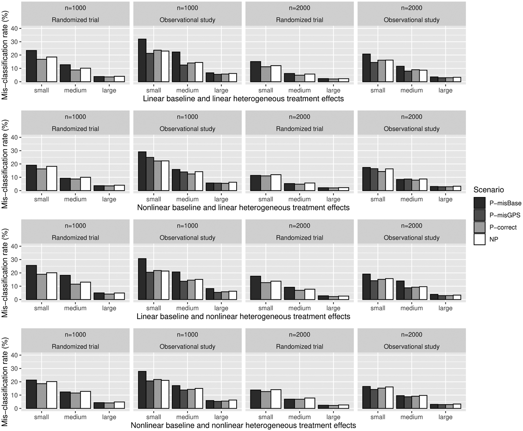
Misclassification rate (%) of identified subgroup based on estimated change-plane parameter $\widehat{\theta }$ for continuous outcome. P-misBase, parametric approach with misspecified baseline model; P-misGPS, parametric approach with mis-specified GPS model; P-correct, parametric approach with both baseline model and GPS model correctly specified; NP, nonparametric approach.

4.2. Type I errors and powers of the proposed test for time-to-event outcome

For time-to-event outcome with right censoring, observed time T was generated based on the model (9) in Section 3.2. Two independent covariates X₁ and X₂ and continuous treatment A were generated similarly as in the setting for continuous outcome. The baseline covariate mean function $\mu (\tilde{X})$ was assumed as the following,

$$\text{B1: linear }\mu (\tilde{X})=0.2X_1+0.2X_2\text{, B2: nonlinear }\mu (\tilde{X})=0.1X_1-0.3X_2^2.$$

The baseline hazards λ₀(t) was assumed to be a constant λ₀ and the censoring time C was generated from a uniform distribution on [0, c₀], where λ₀ and c₀ were chosen to yield a censoring rate of 10% or 20%. Here, we summarized the simulation results when the censoring rate was 20% and the results with 10% censoring rate were provided in Web Appendix Tables A.9 and A.10.

The empirical type I errors and powers of the proposed test were presented in Table 3. The angles of estimated change-plane parameters $\widehat{\theta }$ were summarized in Web Appendix Table A.8. We observed a similar pattern that the powers increased with effect size (small, medium, and large) and sample size for both linear and nonlinear ψ(a). Also, the biases and SDs of $\omega \left(\widehat{\theta },{\theta }_0\right)$ both decreased with increasing effect size and sample size, and the magnitude for P-correct was the smallest compared with other scenarios such as P-misBase, P-misGPS, and NP. In Web Appendix Figure B.3, we visualized the misclassification rate and observed that it decreased with increasing effect size and sample size, and the misclassification rates from P-correct had the lowest values in all settings. We observed that the powers of the proposed test under 10% censoring setting were larger than those under 20% censoring setting. As expected, the angle $\omega \left(\widehat{\theta },{\theta }_0\right)$ and the misclassification rates under 10% censoring setting were both smaller than those under 20% censoring setting.

Table 3.

Empirical Type I errors and powers of the proposed test for time-to-event outcome with 20% censoring rate

N	Study type	Baseline model	Scenario	Type I error	Power: linear ψ(a)			Power: nonlinear ψ(a)
					Small	Medium	Large	Small	Medium	Large
1000	RT	Linear	P-misBase	4.5	31.5	95.7	100	37.8	81.1	100
			P-correct	4.7	32.1	96.2	100	38.4	82.2	100
			NP	4.0	29.6	94.2	100	34.7	77.9	100
		Nonlinear	P-misBase	5.1	30.1	95.6	100	36.9	79.4	100
			P-correct	4.9	29.8	95.5	100	36.6	80.5	100
			NP	3.9	27.8	93.2	100	33.8	76.9	100
1000	OS	Linear	P-misBase	3.8	16.6	74.4	99.8	26.5	65.6	100
			P-misGPS	4.1	12.9	66.7	99.5	21.8	56.6	99.1
			P-correct	3.9	18.7	76.7	99.8	27.9	67.3	99.9
			NP	3.4	20.2	69.7	99.3	27.1	62.7	97.6
		Nonlinear	P-misBase	4.3	17.8	74.1	99.7	26.7	65.5	100
			P-misGPS	3.9	20.4	79.0	99.9	31.5	69.6	100
			P-correct	4.5	17.1	75.6	99.8	27.1	66.7	100
			NP	4.1	17.5	70.5	99.5	27.1	61.4	100
2000	RT	Linear	P-misBase	4.3	69.3	100	100	77.6	99.9	100
			P-correct	4.3	69.4	100	100	78.0	99.9	100
			NP	3.6	63.6	100	100	71.9	99.3	100
		Nonlinear	P-misBase	5.2	66.1	100	100	76.5	99.8	100
			P-correct	4.7	67.7	100	100	76.9	99.9	100
			NP	4.0	61.7	100	100	71.4	99.2	100
2000	OS	Linear	P-misBase	4.0	36.5	99.4	100	59.5	97.1	100
			P-misGPS	4.2	30.1	98.5	100	53.0	94.9	100
			P-correct	4.5	38.4	99.2	100	60.7	97.2	100
			NP	3.9	39.3	98.5	100	56.6	95.5	100
		Nonlinear	P-misBase	4.5	38.9	98.7	100	60.2	97.0	100
			P-misGPS	4.6	39.4	99.3	100	61.0	97.4	100
			P-correct	4.2	37.8	98.9	100	59.9	97.0	100
			NP	4.1	37.2	98.1	100	54.4	95.0	100

RT, randomized trial; OS, observational study;

P-misBase, parametric approach with mis-specified baseline model;

P-misGPS, parametric approach with mis-specified GPS model;

P-correct, parametric approach with both baseline model and GPS model correctly specified; NP, nonparametric approach.

5. Data application

We demonstrated the proposed method for subgroup identification and estimation of differential treatment effects through a cross-sectional study conducted within the Health Effects of Arsenic Longitudinal Study (HEALS), a prospective cohort of 11,746 adult participants enrolled between 2000 and 2002 in Bangladesh to investigate the association between inorganic arsenic (As) exposure in drinking water and blood pressure. The dataset consisted of 726 adolescents aged between 14–17 years whose mothers were participants in the HEALS. Adolescents’ urinary As (UAs) level (a biomarker for As exposure) and blood pressure were measured at the time of recruitment, along with other information including adolescents’ age, sex, body mass index (BMI), and education. The primary interest focused on the association between UAs and systolic blood pressure (SBP) in adolescence. The UAs was log-transformed and centered at mean zero, and other continuous variables were centered. The GPS function was assumed to follow a normal distribution truncated at 5^th and 95^th percentiles of the UAs exposure. To have flexible baseline effect modeling, we allowed nonlinear effects for continuous variables and included a nonlinear main effect of UAs as well.

We conducted hypothesis testing to detect whether there existed two subgroups with differential effects of UAs on SBP, considering adolescents’ age, sex, BMI, and education. The value of the test statistic was 14.5, which was calculated based on 30000 grid points of the sphere coordinates. The p-value was 0.008 based on 1000 resamplings, indicating strong evidence of the existence of two subgroups with differential UAs effects.

When the null hypothesis of no subgroup was rejected, another interest was to estimate the differential treatment effects of the identified subgroup. Our proposed tests focused on hypothesis testing of the existence of subgroups with differential treatment effects. In this application, we further considered the estimating approach proposed for the change-plane model by Li et al. (2021), which was a unified approach for estimation of the differential treatment effects. The estimated change-plane parameters were $\widehat{\theta }={(-0.38,0.36,0.41,0.70,0.25)}^T$ corresponding to the intercept, adolescents’ age, sex, BMI, and education. Based on the estimated $\widehat{\theta }$, the size of the identified subgroup was 309 out of the 719 adolescents, excluding adolescents with any missing values in the covariates. The estimated UAs effects were presented in Figure 2. We visualized the characteristics of the identified subgroup in Figure 3. Based on the estimated change-planes (Figures 3(a) and 3(b)) and the 2D scatter plots (Figures 3(c) and 3(d)), we observed that most adolescents in the high-risk subgroup (subgroup 1) had higher BMI values. The results were consistent with the findings from Chen et al. (2019) that a higher BMI is susceptibility to cardiovascular effects of arsenic exposure. Compared to the moderate effect of UAs on SBP in total sample population, the effect of increasing UAs on SBP was stronger in the high-risk subgroup (subgroup 1), indicating adolescents from the subgroup 1 were more sensitive to the effect of UAs, while the effect of UAs in the low-risk subgroup (subgroup 2) was less significant. As one major importance, our proposed method verified the existence of meaningful subgroups in the HEALS population by conducting formal hypothesis testing and further validated consistent thresholds to define the subgroups without any prespecified cutoff values.

Figure 2.

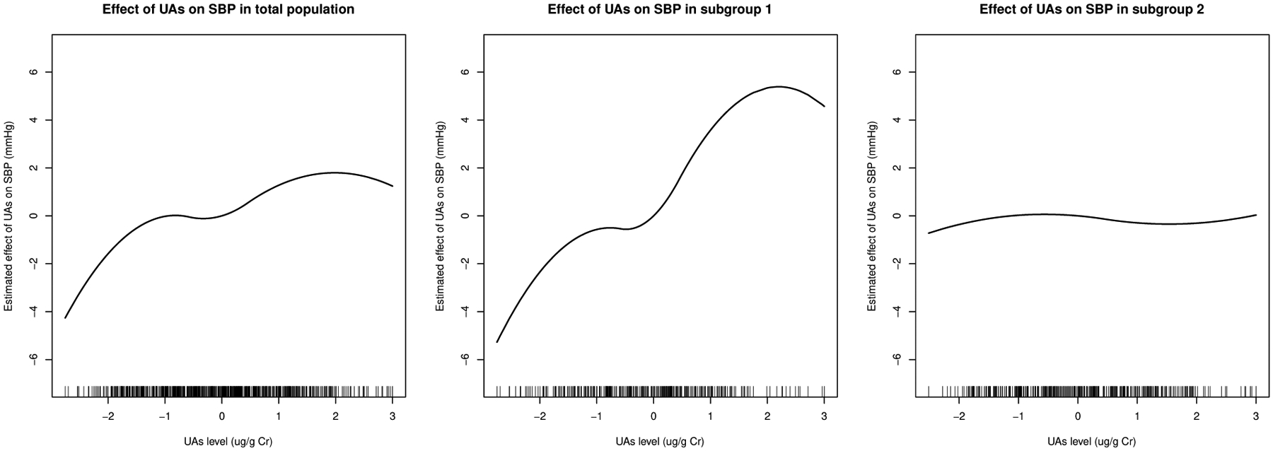
Estimated effect of urinary arsenic exposure UAs on systolic blood pressure (SBP) in total population (left), subgroup 1 (middle), and subgroup 2 (right).

Figure 3.

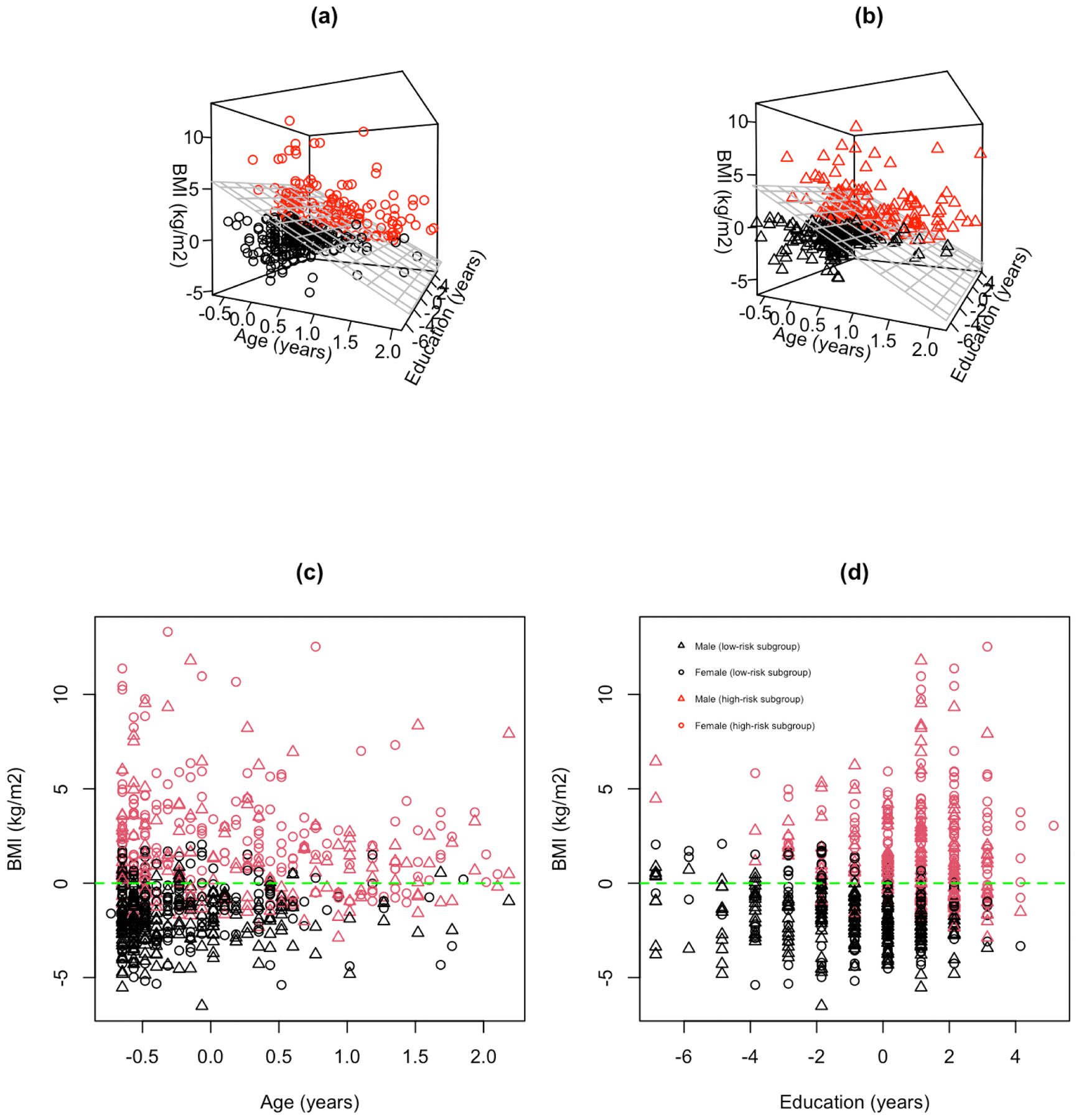
Scatter plots of identified high-risk subgroup (red) and low-risk group (black): (a) females with estimated threshold (gray grid plane) based on $I\left({\widehat{\theta }}^{T}X⩾0\right)$. (b) males with estimated threshold (gray grid plane) based on $I\left({\widehat{\theta }}^{T}X⩾0\right)$. Covariates of BMI, age, and education were all centered. (c) total population in age versus BMI with zero horizontal line (green dashed line). (d) total population in education versus BMI with zero horizontal line (green dashed line).

6. Discussion

In this paper, we proposed a double-robust test procedure for detecting subgroups with differential treatment effects and focused on the continuous treatment (or exposure) setting. The asymptotic distributions of the proposed test statistic under both the null and local alternative hypotheses were established. We further extended the proposed test to handle outcomes from the exponential family of distributions and time-to-event outcome with right censoring. In addition, nonparametric estimation approaches were provided.

In our simulations, the average computational time was less than 2 minutes for a study with two independent covariates, 5000 grid points, and sample size of 2000. The computation burden increases significantly, however, when the number of covariates and the number of grid points are large. One possible solution is to incorporate a built-in variable selection in the testing procedure since only a small number covariates may be helpful for subgroup detection. When the size of the potential subgroup was small, the finite-sample variance matrix estimate ${\widehat{V}}_n(\theta )$ was sparse and its inverse matrix could be unstable. We restricted the potential subgroup size to be within the range 10%−90% of the total sample population to stabilize the numerical performance. Indeed, if the interest is only in testing the null hypothesis only (without estimating the change-plane parameters θ), an un-normalized test statistic T_n can be considered, which does not require the estimation of ${\widehat{V}}_n(\theta )$.

The proposed change-plane model does not include the main effect of treatment, given the focus on testing the existence of subgroups when there is no overall treatment effect. However, the proposed method can be extended easily to include the main effect of treatment. For a continuous treatment A, one may dichotomize it by its mean or median value into a binary treatment. We evaluated the type I errors and powers of the method from Fan et al. (2017) by implementing the dichotomization and further compared it with our proposed approach. Under a linear treatment effect setting, Fan’s method performed well as the linear effect can be captured by the coefficient and a binary treatment. However, under nonlinear non-monotonic treatment effect settings, such as quadratic form, Fan’s approach had low power rejecting the null.

Although we focus on continuous treatment in this paper, as one reviewer mentioned, categorical treatment A is also common in reality. If treatment A is categorical, a multinomial logistic regression model can be considered for modeling the GPS function π(a). Currently, our proposed method is mainly focusing on treatment or exposure measured at a fixed time point. Another extension is to handle a time-dependent treatment or exposure, and the research question is towards identifying a subgroup with cumulative differential effects, of which is a more practical direction in environmental health study. Although our manuscript focuses on the detection of subgroups with differential treatment effects, estimation of differential treatment effects is often of great interest and warrants further investigation. Characterizing the differential treatment effects, along with the profiles of identified subgroups, helps in the understanding of heterogeneity among the population.

Appendix

Regularity conditions

Assume that ψ(a) can be well approximated by a fixed number of spline functions. To establish the asymptotic results given in Theorem 1 and 2, we assume the following regularity conditions.

(C1) Equations E[S₂(X, Y; β)] = 0 and E[S₃(X, A; γ)] = 0 have unique solutions β₀ and γ₀, respectively, and the solutions are in a compact set of the parameter space.

(C2) We have

$$\sqrt{n}\left(\widehat{\beta }-{\beta }_0\right)=-C_1^{-1}{n}^{-1/2}\sum _{i=1}^n{S}_2\left(X_i,Y_i;{\beta }_0\right)+o_p(1),$$

$$\sqrt{n}\left(\widehat{\mathit{\gamma }}-{\mathit{\gamma }}_0\right)=-C_2^{-1}{n}^{-1/2}\sum _{i=1}^n{S}_3\left(X_i,A_i;{\gamma }_0\right)+o_p(1),$$

where C₁ = E[∂S₂(X, Y; β)/∂β^T|_β=β0], $C_2=\text{E}\left[\partial S_3(X,A;\gamma )/\partial {\gamma }_{\gamma ={\gamma }_0}^T\right]$, and both are finite and positive definite deterministic matrices.

(C3) The function S₁(X, Y, A, η; θ) is twice continuously differentiable with respect to η, where η = (β^T, γ^T)^T, and has bounded first and second derivatives.

(C4) The function E[{Y – μ(X; β)}²] is uniformly bounded in β.

(C5) We have 0 < P(θ^T X ⩾ 0) < 1 for any θ ∈ Θ.

Data Availability Statement

The data are not publicly available due to privacy or ethical restrictions. Restrictions apply to the availability of the application data, which were used under permission for this paper.

References

- Andrews DWK (2001). Testing When a Parameter Is on the Boundary of the Maintained Hypothesis. Econometrica 69, 683–734. [Google Scholar]
- Assmann SF, Pocock SJ, Enos LE, and Kasten LE (2000). Subgroup analysis and other (mis)uses of baseline data in clinical trials. Lancet 355, 1064–1069. [DOI] [PubMed] [Google Scholar]
- Bonetti M and Gelber RD (2004). Patterns of treatment effects in subsets of patients in clinical trials. Biostatistics 5, 465–481. [DOI] [PubMed] [Google Scholar]
- Cai T, Tian L, Wong PH, and Wei LJ (2011). Analysis of randomized comparative clinical trial data for personalized treatment selections. Biostatistics 12, 270–282. [DOI] [PMC free article] [PubMed] [Google Scholar]
- Chen G, Zeng D, and Kosorok MR (2016). Personalized dose finding using outcome weighted learning. Journal of the American Statistical Association 111, 1509–1521. [DOI] [PMC free article] [PubMed] [Google Scholar]
- Chen Y, Wu F, Liu X, Parvez F, LoIacono NJ, Gibson EA, Kioumourtzoglou M, Levy D, Shahriar H, Uddin MN, Islam T, Lomax A, Saxena R, Sanchez T, Santiago D, Ellis T, Ahsan H, Wasserman GA, and Graziano JH (2019). Early life and adolescent arsenic exposure from drinking water and blood pressure in adolescence. Environmental Research 178, 108681. [DOI] [PMC free article] [PubMed] [Google Scholar]
- Costa S, Ferreira J, Silveira C, Costa C, Lopes D, Relvas H, Borrego C, Roebeling P, Miranda AI, and Teixeira JP (2014). Integrating health on air quality assessment—review report on health risks of two major European outdoor air pollutants: PM and NO2. Journal of Toxicology and Environmental Health, Part B 17, 307–340. [DOI] [PubMed] [Google Scholar]
- Davies RB (1987). Hypothesis Testing when a Nuisance Parameter is Present Only Under the Alternatives. Biometrika 74, 33–43. [Google Scholar]
- Fan A, Song R, and Lu W (2017). Change-Plane analysis for subgroup detection and sample size calculation. Journal of the American Statistical Association 112, 769–778. [DOI] [PMC free article] [PubMed] [Google Scholar]
- Farrell MH, Liang T, and Misra S (2021). Deep neural networks for estimation and inference. Econometrica 89, 181–213. [Google Scholar]
- Foster JC, Taylor JM, and Ruberg SJ (2011). Subgroup identification from randomized clinical trial data. Statistics in Medicine 30, 2867–2880. [DOI] [PMC free article] [PubMed] [Google Scholar]
- Hirano K and Imbens G (2004). The propensity score with continuous treatments. In Gelman A. and Meng X-L, editors, Applied Bayesian modeling and causal inference from incomplete-data perspectives. Wiley Series in Probability and Statistics, Hoboken, NJ: Wiley, pp. 73–84. [Google Scholar]
- Hirvonen A (1995). Genetic factors in individual responses to environmental exposures. Journal of Occupational and Environmental Medicine 37, 37–43. [DOI] [PubMed] [Google Scholar]
- Huang Y, Cho J, and Fong Y (2020). Threshold-based subgroup testing in logistic regression models in two-phase sampling designs. Journal of the Royal Statistical Society: Series C (Applied Statistics) 70, 291–311. [DOI] [PMC free article] [PubMed] [Google Scholar]
- Imai K and Ratkovic M (2013). Estimating treatment effect heterogeneity in randomized program evaluation. The Annals of Applied Statistics 7, 443–470. [Google Scholar]
- Imai K and van Dyk DA (2004). Causal inference with general treatment regimes. Journal of the American Statistical Association 99, 854–866. [Google Scholar]
- Kang S, Lu W, and Song R (2017). Subgroup detection and sample size calculation with proportional hazards regression for survival data. Statistics in Medicine 36, 4646–4659. [DOI] [PMC free article] [PubMed] [Google Scholar]
- Kent DM, Steyerberg E, and Klaveren DV (2018). Personalized evidence based medicine: predictive approaches to heterogeneous treatment effects. British Medical Journal 363, k4245. [DOI] [PMC free article] [PubMed] [Google Scholar]
- Kosnik MB, Enroth S, and Karlsson O (2021). Distinct genetic regions are associated with differential population susceptibility to chemical exposures. Environment International 152, 106488. [DOI] [PubMed] [Google Scholar]
- Li J, Li Y, Jin B, and Kosorok MR (2021). Multithreshold change plane model: estimation theory and applications in subgroup identification. Statistics in Medicine 40, 3440–3459. [DOI] [PMC free article] [PubMed] [Google Scholar]
- Li J, Yue M, and Zhang W (2019). Subgroup identification via homogeneity pursuit for dense longitudinal/spatial data. Statistics in Medicine 38, 3256–3271. [DOI] [PubMed] [Google Scholar]
- Lipkovich I, Dmitrienko A, and B D’Agostino R Sr (2017). Tutorial in biostatistics: data-driven subgroup identification and analysis in clinical trials. Statistics in Medicine 36, 136–196. [DOI] [PubMed] [Google Scholar]
- Park H, Petkova E, Tarpey T, and Ogden RT (2021). A single-index model with a surface-link for optimizing individualized dose rules. Journal of Computational and Graphical Statistics 31, 553–562. [DOI] [PMC free article] [PubMed] [Google Scholar]
- Robins J and Rotnitzky AG (2001). Comment on the Bickel and Kwon article, ‘Inference for semiparametric models: some questions and an answer’. Statistica Sinica 11, 920–936. [Google Scholar]
- Shen J and He X (2015). Inference for subgroup analysis with a structured Logistic-Normal mixture model. Journal of the American Statistical Association 110, 303–312. [Google Scholar]
- Song X and Pepe MS (2004). Evaluating markers for selecting a Patient’s Treatment. Biometrics 60, 874–883. [DOI] [PubMed] [Google Scholar]
- Tsiatis AA (2006). Semiparametric Theory and Missing Data. Springer, New York. [Google Scholar]
- Wang J, Li J, Li Y, and Wong WK (2019). A model-based multithreshold method for subgroup identification. Statistics in Medicine 38, 2605–2631. [DOI] [PubMed] [Google Scholar]
- Wang R, Lagakos SW, Ware JH, Hunter DJ, and Drazen JM (2007). Statistics in medicine-reporting of subgroup analyses in clinical trials. The New England Journal of Medicine 357, 2189–2194. [DOI] [PubMed] [Google Scholar]
- Wei S and Kosorok MR (2018). The change-plane Cox model. Biometrika 105, 891–903. [DOI] [PMC free article] [PubMed] [Google Scholar]
- Wu R, Zheng M, and Yu W (2016). Subgroup analysis with time-to-event data under a Logistic-Cox mixture model. Scandinavian Journal of Statistics 43, 863–878. [Google Scholar]
- Zhao L, Tian L, Cai T, Claggett B, and Wei LJ (2013). Effectively selecting a target population for a future comparative study. Journal of the American Statistical Association 108, 527–539. [DOI] [PMC free article] [PubMed] [Google Scholar]
Associated Data
This section collects any data citations, data availability statements, or supplementary materials included in this article.
Supplementary Materials