

Abstract

MILD (moderate and intense low-oxygen dilution) combustion is a highly promising technology to deliver clean and efficient thermal energy. However, because of its unconventional reaction nature, the optimization of the MILD combustion in various industrial burners is still challenging, for which the design tool based on accurate and cost-effective numerical simulation is most desirable. To this end, the tabulated chemistry approach (TCA) is thoroughly assessed for the modeling of MILD combustion by simulations of the Adelaide Jet in Hot Coflow (JHC) burner. The sensitivities to the submodel accounting for the scalar micromixing and the canonical flame configurations (i.e., flamelet and PSR-based reactors), being relevant for MILD regime characterization in TCA, are studied. It is found that the scalar mixing enhanced through the dynamic adjustment of model parameter Cs leads to an improved prediction, and the optimal value of Cs = 8 is identified for the current flames. The proper parametrization of the detailed chemical structures in TCA is found to affect the accurate prediction of the MILD flame profiles, especially the mass fraction of minor species (e.g., OH, CO). Furthermore, the endothermic reaction path of O + C2H2 ⇒ CO + CH2 is indicated as the main contributing step to the disparities in the CO predictions. This implies that the multiple reaction regimes in complex MILD burning should be accounted for by the use of either flamelet or PSR structures, depending on the local microscale diffusion/chemistry competitions. Overall, the results highlight the influential role of multiscale mixing and its intercoupling with the finite-rate chemistry, the accurate determination of which is important for MILD combustion modeling.
1. Introduction
The energy shortage and environmental concerns raise the need for the development of a clean and efficient energy generator powered by combustion. As one attractive solution, MILD (moderate and intense low-oxygen dilution) combustion promises to achieve high thermal efficiency and, at the same time, extremely low emissions of carbon monoxide and nitric oxides.1,2 In practice, this combustion mode is commonly achieved through the recirculation of flue gas, which provides both the high-temperature preheating of reactants to be above the autoignition temperature and the dilution of combustion air such that the heat release is moderate with a small temperature increase (lower than the self-ignition temperature).1 In this way, the heat from exhaust gas is reused, and the appearance of a local reaction zone with a high temperature peak is alleviated, leading to a significant reduction in NOx pollution. Owing to such a beneficial feature, MILD combustion is gaining great interest in the exploration of its fundamental aspect experimentally and numerically, in order to promote its applications for various burners (i.e., industrial furnace3 and gas turbine4) and fuels such as gas, oil,2 coal,5 or renewable biomass.4
By employing the Jet in Hot Coflow (JHC) burner to emulate the MILD condition, Dally et al.6 measured a series of CH4/H2 blended fuel flames under varying degrees of dilution of oxidant stream. They reported that although the decreased oxygen content would lead to the decline of peak flame temperature, an easier establishment of MILD combustion was observed at the lower O2 level. Evans et al.7 found that the oxidant temperature and O2 concentration have also a synergistic effect on the flame stabilization. Their experimental observations of laminar MILD methane flame suggested that the stabilization of flames in the 1315 K coflow with changing O2 level was controlled by different mechanisms, and a similar stabilization mechanism existed within flames under the higher temperature of 1385 K. The author further highlighted the importance of the oxidant composition such as the OH radical which was found to enhance a MILD CH4 reaction zone by increasing the CH3 oxidation. Similarly, the impact of carrier gas on the structure of MILD flame with prevaporized ethanol fuel was reported by Ye,8 and the flame carried by nitrogen instead of air had a more uniform temperature distribution.
Apart from the inlet species and temperature conditions, the mixing between the fuel and diluted oxidant stream was deemed to also play a vital role in achieving the MILD combustion.1,9−12 Plessing et al.9 investigated the combustion features of a reversed flow combustor via the Rayleigh and OH images. It was found that the MILD reaction zone can only be observed where the unburnt mixture was heated up by the recirculated exhaust gases above 950 K. Another study on a multiple jet combustion burner10 reported that the temperature above autoignition and the high dilution rate were necessary conditions for the realization of stable combustion and low CO emissions in a MILD burner. To satisfy these conditions, the effective mixing was required. Derudi et al.11 found that when hydrogen was present in the fuels, a higher nozzle velocity should be designed to realize a stable MILD combustion. Li et al.12 also demonstrated the importance of a high fuel-jet momentum rate which was required for burning higher-reactivity fuel such as ethylene in comparison to natural gas and liquefied petroleum gas, for MILD combustion. After examining the characteristics of MILD combustion of natural gas fired under nonpremixed (NP), partially premixed (PP), and fully premixed (FP) burning modes, Li et al.13 identified the FP burning as the most efficient way to produce the lower emissions since a highest jet momentum rate was attained under this burning condition.
These experimental studies showed the importance of mixing for the realization of MILD combustion. In numerical simulations, this indicates that a proper closure model for mixing is required in order to accurately reproduce its complex interactions with the chemical reactions. For MILD combustion, one of the commonly used combustion models in the literature is the eddy dissipation concept (EDC) owing to its ability to account for the finite-rate chemical effect.14 However, the standard EDC model has limited success in reproducing the main structure of a MILD flame.14−16 De et al.16 assessed the EDC performance in the simulation of the Delft JHC burner. The computation from the standard model appeared to overestimate the flame temperature with an earlier ignition; however, an improved prediction was attained by adjustment of the model coefficient Cτ relating to the mixing time scale from 0.4083 to 3. The same observations and adjustment of EDC model constant were also reported in the simulations of the Adelaide JHC flames with methane/hydrogen and ethylene fuels.17,18 Those EDC modifications implied that an improved prediction needs to deal with the specific nature of the reaction zone with strong turbulence–chemistry coupling in the MILD regime.15 Parente et al.19 thus revisited the derivation of the EDC model constants, for which a new formulation was proposed in order to explicitly take into account the distributed nature of the MILD flame structure by use of the local Reynolds and Damköhler numbers. However, given the improvement observed by change of the model constants, the failure in simulating the MILD flame with local extinction still existed for EDC modeling.20 On the contrary, the transported PDF (tPDF) model outperformed the prediction of flame with the local intermittent extinction, albeit with changing of the tPDF mixing constant Cϕ from the default value of 2 to 5.20 Nonetheless, the implementation of the tPDF model is impeded due to the further increased computational cost associated with the inclusion of the detailed kinetic scheme that is indispensable to capture the MILD flame structure correctly.21 Thus, shown from the reviewed studies, for the MILD combustion, the accurate prediction also highly depends on the treatment of the mixing scale, and meanwhile, cost-effective modeling remains a challenge.
In this regard, the tabulated chemistry approach (TCA) like the flamelet model22 provides a promising alternative to include the detailed chemistry at a reduced computational cost. However, although this approach has been extensively investigated in the conventional flames,23−25 works focusing on the modeling of MILD combustion are still rare. In an early work,26 the flamelet approach was extended to a three-stream formulation by adding another mixing variable, and this new formulation showed a good LES prediction of a methane/hydrogen MILD jet flame. Lamouroux et al.27 extended the tabulated chemistry approach to account for the effects of gas dilution and heat loss, and a general good prediction of measurements for the reversed flow MILD combustor was reported. Abtahizadeh et al.28 also discussed the influence of molecular differential diffusion by inclusion of this effect in a flamelet-based TCA model, which, compared with the DNS data, showed its attractive ability in the modeling of the hydrogen enriched MILD flames. While successful, flamelet-based TCA is still questioned for its applicability because of the model assumption that the turbulent flame front is assumed to be a laminar thin flame. Although the flamelet-like structures were reported in some previous studies of the MILD burner with moderate Damköhler number,13,29 a distributed reaction zone was thought to be another proper representative of the combustion operating in MILD condition.30 Therefore, the tabulated chemistry established based on an unsteady perfectly stirred reactor (PSR) has also been developed for the simulations of MILD flames.31 Recently, Chitgarha and Mardani32 evaluated the steady flamelet model in the simulation of CH4/H2 JHC burner; compared to the EDC modeling, a lower accuracy of the flamelet predictions was observed. This conclusion, however, is not general since those steady flamelet applied in their study was parametrized only by the scalar dissipation rate χ, instead of the reaction progress variable that is deemed to better the prediction of flame structures under a various condition including the local extinction.23,26
Therefore, with the aforementioned background, it is of great interest to better the understanding of the fundamental mixing process and its interaction with the chemistry in MILD combustion, and meanwhile, to establish the accurate and cost-effective modeling strategy. The latter one is the most desirable, in particular for the design and optimization of industrial boilers and furnaces operating in the MILD condition. By addressing these aspects, the major objective of this study is to have a thorough assessment of the tabulated chemistry approach in the context of MILD flame simulation; the influence of the mixing model and tabulation strategy, i.e., the choice of different prototype flame structures, on the prediction of MILD flame will be investigated. To the best of the authors’ knowledge, this kind of study has not been yet performed. In addition, since there is a general need of a proper inclusion of detailed chemical kinetics for the accurate prediction of MILD combustion, the impact of different kinetic schemes is also examined, followed by a study of the fuel oxidation pathway in different flame conditions. This allows to gather the valuable insights on the unconventional MILD nature in terms of chemical reaction dynamics. The following sections are organized as the gas equations and TCA description will be presented in the section 2, after which the experimental flames and the numerical setup are given. Then the results and conclusions are provided in sections 4 and 5, respectively.
2. Mathematical Method
2.1. Governing Equations
In this work, the flame structure is predicted using the chemical structures pregenerated by the tabulation approaches, in a combination with the RANS equations. The turbulent flame is assumed to be composed of the flame structures that are parametrized typically by a reduced set of controlling variables, i.e., the mixture fraction Z and reaction progress variable C. Then, the governing equations of the mass and momentum as well as Z and C are solved as25,33
| 1 |
| 2 |
| 3 |
| 4 |
where  is the pressure,
  is the Reynolds stresses, and
 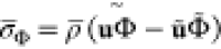 (Φ = {Z, C}) are the terms of turbulent scalar flux, modeled as
  , where the Schmidt number Sct is assigned with 0.7. The eddy viscosity
μt is prescribed using
, where the Schmidt number Sct is assigned with 0.7. The eddy viscosity
μt is prescribed using 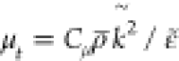 (Cμ =
0.09) in a context of standard k-ε turbulence
model. The mixture fraction Z describes the mixing
state between the fuel and oxidizer, and the reaction progress of
mixture, denoted by the variable C, is defined here
as the normalized mass fraction of species,
(Cμ =
0.09) in a context of standard k-ε turbulence
model. The mixture fraction Z describes the mixing
state between the fuel and oxidizer, and the reaction progress of
mixture, denoted by the variable C, is defined here
as the normalized mass fraction of species,  ,23
,23
| 5 |
and  represents the equilibrium state of reactant
mixture and is a function of Z.
represents the equilibrium state of reactant
mixture and is a function of Z.  denotes the initial mixing state determined
by the inlet boundary condition. The reaction source term
denotes the initial mixing state determined
by the inlet boundary condition. The reaction source term  in eq 4 is modeled following ref (25) and is taken from the
chemical library that
is pregenerated by the tabulated chemistry approaches.
in eq 4 is modeled following ref (25) and is taken from the
chemical library that
is pregenerated by the tabulated chemistry approaches.
2.2. Tabulated Chemistry Approach
In the
tabulation approach, the full set of thermo-chemical scalars in the
flowfield are retrieved from the chemical table that is determined
by a proper reactor model. Usually, the one-dimensional premixed or
diffusion flame is applied by the flamelet modeling, depending on
the burning regime.25 Flamelet method has
been a success in the simulation of the various (gas or liquid) flames.
In the DNS study of MILD combustion, Minamoto et al.30 observed that, associated with the intense mixing, the
reaction zones interact with each other frequently, leading to the
appearance of distributed combustion, thereby they suggested a homogeneous
perfectly stirred reactor (PSR)34 to account
for the MILD flame structure. Although the performance of these different
flame element configurations is still unclear, in general, by the
use of Z and C, the parametrization
strategy for the flame composition  is
is
| 6 |
Here the probability
density function  is modeled as the product of the marginal
PDF of the variables Z and C which
are both assumed to follow a beta distribution in this work. To evaluate
the PDF, the variances of mixture fraction,
is modeled as the product of the marginal
PDF of the variables Z and C which
are both assumed to follow a beta distribution in this work. To evaluate
the PDF, the variances of mixture fraction,  and progress variable,
  are calculated by the
solution of their
conservation equations,33
are calculated by the
solution of their
conservation equations,33
| 7 |
| 8 |
In the above equations, the constant Cg equals 2.86, and the turbulent
scalar flux of  and
and  is determined in the
same way as eq 3 by use
of the eddy diffusivity
hypothesis. The scalar dissipation rate of mixture fraction
is determined in the
same way as eq 3 by use
of the eddy diffusivity
hypothesis. The scalar dissipation rate of mixture fraction  in the turbulent flame is typically estimated
relying on a proportionality to the turbulent mixing time scale τmix as35
in the turbulent flame is typically estimated
relying on a proportionality to the turbulent mixing time scale τmix as35
| 9 |
and τmix is commonly determined by a relation to the integral time scale,
| 10 |
with the coefficient Cs, in general, assigned as 2.0.35 This value, however, is not universal and essentially it varies depending on the flame considered; to a large extent, it influences the performance of flamelet modeling of flames that deviate from the traditional combustion regime.36,37 For instance, in the transported PDF simulation of a MILD methane jet flame, Christo and Dally20 found that a stabilized flame was only achieved when a modified Cs = 5.0 was adopted.
Another definition of the mixing time τmix was proposed in several previous studies.38−40 Based on the energy cascade theory, the mixing process can be determined by the Kolmogorov scale, and the mixing time scale is limited by the residence time as38
| 11 |
where ν is the kinematic viscosity and the default value of Cτ is 0.4083.38 In addition, by considering the geometric mean of the integral and Kolmogorov mixing time scale, Li et al.39 used the formulation
| 12 |
which performed well in the partially stirred reactor modeling of a MILD jet flame. This is similar to the formulation described in ref (40) derived using the RNG theory, as
| 13 |
On the other hand, the simple closure
model for  is often retained, following the assumption
that the mixing of C can be determined by the lifetime
of turbulent motions same as the passive scalar, i.e., the mixture
fraction, as22
is often retained, following the assumption
that the mixing of C can be determined by the lifetime
of turbulent motions same as the passive scalar, i.e., the mixture
fraction, as22
| 14 |
where Cc denotes the
ratio about the mixing time scales between the Z and C, and it is commonly taken as a
constant of 1.0.35 Ihme et al.41 pointed out, however, that in the flame with
distinctly separate mixing and reaction regions, the reactive scalar
would experience the variation in the time scale ratio, for which 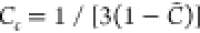 was proposed. To account for the various
flame regime, other algebraic models of
was proposed. To account for the various
flame regime, other algebraic models of  have also been developed42 by considering the balance of the dominant terms of the
transport equation for a scalar variance equation.
have also been developed42 by considering the balance of the dominant terms of the
transport equation for a scalar variance equation.
Since in the tabulated chemistry approach, the scalar dissipation rate plays a pivotal role in modeling of the micromixing process, its influence or the role of micromixing on the prediction of specific flame structures in MILD regime is first investigated.
3. Configuration
3.1. Experimental Setup
In the present work, the jet flames measured based on the Adelaide JHC burner6 are simulated, which consist of a central fuel nozzle of diameter Dj = 4.25 mm and a surrounding annulus hot-coflow. The whole burner was mounted in a wind tunnel providing the coaxial air-flow. The fuel stream is the mixture of methane/hydrogen in a volumetric ratio of 1:1, and has a bulk velocity of U0 = 70 m/s. The hot-coflow with the mean velocity of 3.2 m/s is the combustion products diluted with air and nitrogen, leading to the three (HM1, HM2, and HM3) cases corresponding to O2 mass levels of 3%, 6%, and 9%, respectively. The temperatures of the fuel and coflow streams are 305 and 1300 K, respectively. Listed in Table 1 are the details of jet boundary conditions for the two extreme cases of HM1 and HM3 that are considered in the present study.
Table 1. Boundary Condition of Jet Flame HM1 and HM3 at Inlet6.
| Fuel | Hot coflow (HM1) | Hot coflow (HM3) | |
|---|---|---|---|
| Temperature [K] | 305 | 1300 | 1300 |
| Bulk Velocity [m/s] | 70 | 3.2 | 3.2 |
| Compositions [-] | YCH4 = 0.889 | YO2 = 0.03 | YO2 = 0.09 |
| YH2 = 0.111 | YN2 = 0.85 | YN2 = 0.79 | |
| YH2O = 0.065 | YH2O = 0.065 | ||
| YCO2 = 0.055 | YCO2 = 0.055 |
3.2. Numerical Procedure
The steady-state RANS equations are discretized by a finite volume method, and the SIMPLE algorithm is utilized for the pressure–velocity coupling. The turbulent flow is simulated using the modified k – ϵ model with the value of Cϵ1 = 1.6 such that an improved prediction can be obtained for the round jet.43 All computations presented have been performed using the FLUENT code with the user defined function (UDF)44 which includes the use of DEFINE macros such as DEFINE_SOURCE, DEFINE_PROPERTY, DEFINE_ DIFFUSIVITY, etc. A 2D axisymmetric computational domain extending to 500 mm and 210 mm in stream-wise and transverse directions, respectively, is adopted, and it is discretized into 45,600 cells with the nonuniform grids concentrated in the flame region, see Figure 1(a). A similar mesh setup has been verified in many other studies.45,46
Figure 1.

(a) Schematic of the computational domain; (b) the S-shaped curve and the reaction rate in Z and C space obtained from FPV and PSR library for HM1 (α = 1.0 × 10⁴) and HM3 (α = 1.0 × 10³) cases.
The combustion chemistry is modeled using the pretabulated chemistry tables, which allow the inclusion of a detailed chemical mechanism. As indicated by ref (30), the flame in the MILD regime features a close interplay between the turbulence and finite-rate chemistry, and the adoption of the detailed mechanism is essential to capture the flame structures. In this work, to further assess the influence of chemistry within the framework of the tabulation approach, five different mechanisms, i.e., the DRM-22 (22 species),47 GRI2.11 (49 species),48 USC2.0 (111 species),49 KONNOV (127 species),50 and AramcoMech2.0 (493 species)51 are chosen. Among these schemes, the DRM-22 originating from GRI1.2 has been often employed in EDC simulations due to the reduced size,15,17 and it serves as a reference scheme for the comparison of other detailed mechanisms. The steady diffusion flame module in FlameMaster52 is used to generate the structured chemistry table following the flamelet/progress variable (FPV) method,25 while the PSR tabulation is acquired based on the PSR reactor of CHEMKIN solver.53 In the table, the uniformly distributed mesh with the grid numbers of 92 and 51 are used for the coordinate variables Z and C, respectively, and the geometric growth law is adopted for the discretization of variances Zv and Cv with the grid number of 18.
Figure 1(b) shows the calculated S-shaped curves and the plots of reaction rate for HM1 and HM3 that are obtained from the generated libraries by the FPV and PSR reactor. The S curve consists of the upper and lower branches. If χst is increased, the burning state is traversed to the lower branch until the extinction strain rate is reached. In the HM1 case the extinction strain rate is absent, which is in accordance with the previous observation54 that a heavily diluted and preheated condition can lead to a smooth transition from reacting solution to the nonreacting state. This indicates that the HM1 case is more prone to burn in the MILD regime than the HM3 case. As to the S curve computed from PSR, the abscissa axis is the inverse of the residence time (τres) scaled by a factor of α. It can be seen that in these two flame cases, FPV and PSR calculations merge into the similar curves, which implies that in terms of the function between flame peak temperature and the mixing time scale, this two different canonical flame configurations show the same flame dynamics.
In addition, compared to the HM3 with stoichiometric mixture fraction Zst around 0.0199, the HM1 with a lower oxygen level is characterized by a smaller region of intense reaction in the Z – C space, and the flame moves further to the oxidant side leading to Zst = 0.0067. Furthermore, the flamelet FPV library features an extended distribution in the Z direction in contrast to a broader distribution denoted by the PSR model in the C direction. This is because the diffusion transport in Z space is included in the flamelet equation, whereas for a specific mixture, the thermochemical scalars in the PSR reactor are affected only by the mixture residence time.
In the end, the generated structured chemical tables are loaded in the FLUENT computation through a bespoke program applying the UDF library and UDS function that includes the solution of additional eqs 3, 4, 7, and 8. The mixture fraction at the fuel and coflow inlets are set to be 1.0 and 0.0, respectively. The inlet value of C at the fuel side is 0.0 and for the hot-coflow, this value is 1.0. The turbulent kinetic energy at the fuel and coflow boundaries are taken to be 60 and 1.8 m2/s2,55 respectively.
4. Results and Discussion
4.1. Assessment of Scalar Mixing Model
In this section,
first the key process of scalar mixing, in the RANS-flamelet
simulation combined with the GRI2.11 scheme and different closure
models of  and
and  , is investigated by considering the nine
computational cases listed in Table 2. The details of different models have been described
in the above section. Here to account for the variation in the combustion
regime,12,25 the algebraic expression (SDR3) of Kuan
et al.42 for the scalar dissipation rate
, is investigated by considering the nine
computational cases listed in Table 2. The details of different models have been described
in the above section. Here to account for the variation in the combustion
regime,12,25 the algebraic expression (SDR3) of Kuan
et al.42 for the scalar dissipation rate  is also evaluated, which has a relation
to the Kolmogorov turbulent velocity νk = (νϵ)1/4 and laminar
flame speed SL. The model
constant
is also evaluated, which has a relation
to the Kolmogorov turbulent velocity νk = (νϵ)1/4 and laminar
flame speed SL. The model
constant  and Cklv are set to
1.2 and 4, respectively. The unburnt mixture density
ρu and SL are determined from the chemical library precalculated
by a laminar premixed flame.
and Cklv are set to
1.2 and 4, respectively. The unburnt mixture density
ρu and SL are determined from the chemical library precalculated
by a laminar premixed flame.
Table 2. Computational Cases to Assess the Scalar Mixing Effect.
| Case | χ̃Z closure | χ̃C closure | τmix model | |||
|---|---|---|---|---|---|---|
| SDR1 |
 , Cc = 1 , Cc = 1 |
|||||
| SDR2 |
 , , 
|
|||||
| SDR3 | ||||||
| SDR4 |
 , Cc = 1 , Cc = 1 |
|||||
| SDR5 |
 , Cc = 1 , Cc = 1 |
|||||
| SDR6 |
 , Cc = 1 , Cc = 1 |
|||||
| SDR7 |
 , Cc = 1 , Cc = 1 |
|||||
| SDR8 |
 , Cc = 1 , Cc = 1 |
|||||
| SDR9 |
 , Cc = 1 , Cc = 1 |
Shown in Figure 2 is the comparison of the computed temperature
and
main species H2O mass fraction with the measurements for
the simulation cases
from SDR1 to SDR6. Generally, for cases with different closures of  , i.e., SDR1, SDR2, and SDR3, a marginal
influence on prediction is observed, where the SDR2 and SDR3 only
lead to a relative 1.5% decrease and 1.0% increase in peak temperature,
respectively, compared to the SDR1. A salient difference is observed,
on the other hand, in the prediction of species mass fraction, especially
for case SDR2. Together with the observation indicated by Figure 3 of mass fraction
of CO and OH, SDR2 predicts a spatially narrower distribution of YCO and
, i.e., SDR1, SDR2, and SDR3, a marginal
influence on prediction is observed, where the SDR2 and SDR3 only
lead to a relative 1.5% decrease and 1.0% increase in peak temperature,
respectively, compared to the SDR1. A salient difference is observed,
on the other hand, in the prediction of species mass fraction, especially
for case SDR2. Together with the observation indicated by Figure 3 of mass fraction
of CO and OH, SDR2 predicts a spatially narrower distribution of YCO and  , while SDR3 shows a comparable result with
SDR1. This may be because although the present JHC flame shows a slight
lifted-off behavior near the flame base,6,56 the effect
of mixing in preignition regime on the flame structures is negligible
and this Adelaide MILD flame is prone to be a typical nonpremixed
flame.
, while SDR3 shows a comparable result with
SDR1. This may be because although the present JHC flame shows a slight
lifted-off behavior near the flame base,6,56 the effect
of mixing in preignition regime on the flame structures is negligible
and this Adelaide MILD flame is prone to be a typical nonpremixed
flame.
Figure 2.

Comparison of temperature and species mass fraction  for flames HM1 and HM3 (dots, experiments;
line, computed results of cases SDR1–6) at axial locations X = 30, 60 mm.
for flames HM1 and HM3 (dots, experiments;
line, computed results of cases SDR1–6) at axial locations X = 30, 60 mm.
Figure 3.

Comparison of species mass fraction YCO and YOH for flames HM1 and HM3 (dots: experiments and line: computed results of cases SDR1–6) at the axial locations X = 30, 60 mm.
Furthermore, based on the SDR1 case with the default value of Cs = 2, the computations with Cs = 34−6,8 and 10 (i.e., decreasing the scalar mixing time scale) are performed to study the sensitivity to the variations in parameter Cs. Here, only the cases SDR4, SDR5, and SDR6 (viz. Table 2) are depicted, the results of which obviously deviate from the case SDR1; the predicted temperature increases with the increase of Cs and the computation with a large Cs is closer to the experimental data. The mass fraction of species computed with the large Cs, especially for YCO, also shows a spatial distribution extended toward to the inner side of the flame and this well captures the experimental trend. As indicated by refs (57 and 58), MILD combustion is characterized by a specific nature of a uniform and distributed reaction zone owing to the intense mixing. The improvement in the prediction by varying Cs could thus be explained by the fact that the elevated Cs results in an enhanced mixing with smaller τmix, which helps grow the reaction. This is also confirmed by the increasing reaction rate with smaller mixing time shown in Figure 1(b). This effect is also noticed by Mardani 15. In his work, the default parameter in the EDC model was reduced to lower the volume fraction and the mixing time scale, relying on which the reaction evolves to reach a better prediction. This change forces the reaction to move toward the finite-rate condition and on the whole, intensifying the reaction zone, which is compatible with the MILD flame characteristics of distributed and large volume reaction.
Figure 4 shows the
variation of the difference between the computed peak temperature Tmax and the measured one  when the
value of Cs is escalated.
It can be seen that for both
flame cases, the difference decreases as Cs increases; however, the case HM3 seems to be more
sensitive to the changes in parameter Cs. The peak temperature of HM1 at two downstream cross
sections presents a slower but similar variation. This could be due
to the fact that the HM1 flame has a lower oxygen level in the coflow
and operates more like in the MILD zone, leading to a reaction where
the oxygen is the key factor and the fuel is mixed and consumed uniformly
in the space. The plot also shows that with Cs = 8, a much better prediction of flame peak
temperature is obtained. Here, we assume that a universal constant
value of Cs exits for
the different flame regimes, but Cs may vary locally depending on the flow condition, which will
be discussed in the later section.
when the
value of Cs is escalated.
It can be seen that for both
flame cases, the difference decreases as Cs increases; however, the case HM3 seems to be more
sensitive to the changes in parameter Cs. The peak temperature of HM1 at two downstream cross
sections presents a slower but similar variation. This could be due
to the fact that the HM1 flame has a lower oxygen level in the coflow
and operates more like in the MILD zone, leading to a reaction where
the oxygen is the key factor and the fuel is mixed and consumed uniformly
in the space. The plot also shows that with Cs = 8, a much better prediction of flame peak
temperature is obtained. Here, we assume that a universal constant
value of Cs exits for
the different flame regimes, but Cs may vary locally depending on the flow condition, which will
be discussed in the later section.
Figure 4.

Variation of temperature difference,  , between prediction and experiments
when Cs is increased
for flame cases
HM1 and HM3 at axial locations X = 30, 60 mm.
, between prediction and experiments
when Cs is increased
for flame cases
HM1 and HM3 at axial locations X = 30, 60 mm.
Figures 5 and 6 show the comparison of experimental
data and the
predicted results of T and species  , YCO, and YOH for the cases of SDR7, SDR8, and SDR9, which
adopt the different models for the mixing time scale τmix. Despite the similar trend shared by the computations of SDR7 and
SDR8, they both exhibit a better prediction compared to the SDR1.
A best fit against the experimental profiles, however, is obtained
from the prediction in case SDR9 in which the model assumes that the
reaction is controlled by the fine structures. This observation implies
that the flamelet-based modeling of flame in the MILD zone is in favor
of using the time scale model that considers the contribution from
the Kolmogorov scale (or the equivalent diffusive scale) region, where
the mixing is even faster. To show how this affects the local value
of Cs, an equation is
defined as
, YCO, and YOH for the cases of SDR7, SDR8, and SDR9, which
adopt the different models for the mixing time scale τmix. Despite the similar trend shared by the computations of SDR7 and
SDR8, they both exhibit a better prediction compared to the SDR1.
A best fit against the experimental profiles, however, is obtained
from the prediction in case SDR9 in which the model assumes that the
reaction is controlled by the fine structures. This observation implies
that the flamelet-based modeling of flame in the MILD zone is in favor
of using the time scale model that considers the contribution from
the Kolmogorov scale (or the equivalent diffusive scale) region, where
the mixing is even faster. To show how this affects the local value
of Cs, an equation is
defined as
| 15 |
where τmix is modeled by the formulation listed in Table 2 for cases SDR7, SDR8, and SDR9. The Cs calculated dynamically by eq 15 is presented in Figure 7 which compares the Cs radial distribution at cross sections of X = 30 and 60 mm for cases SDR8 and SDR9. As shown, in the case SDR8, the modeled parameter Cs has a value locating between the Cs = 1 and the optimal value of Cs = 8 found in the above analysis. On the other hand, in the most reactive region, the Cs value from SDR9 reaches above the 8 giving its prediction in a better agreement with experiments. However, the results also indicate that a higher Cs does not guarantee a further improvement of predictions.
Figure 5.

Comparison of temperature and species mass fraction  for flames HM1 and HM3 (dots, experiments;
line, computed results of cases SDR1,7,8,9) at axial locations X = 30, 60 mm.
for flames HM1 and HM3 (dots, experiments;
line, computed results of cases SDR1,7,8,9) at axial locations X = 30, 60 mm.
Figure 6.

Comparison of species mass fraction YCO and YOH for flames HM1 and HM3 (dots, experiments; line, computed results of cases SDR1,7,8,9) at axial locations X = 30, 60 mm.
Figure 7.

Radial distribution of parameter Cs (see eq 15) at the axial locations X = 30, 60 mm for flames HM1 and HM3. Vertical axis at the left- and right-hand sides corresponds to the results of SDR9 (black line) and SDR8 (red lines), respectively.
Meanwhile, it is interesting to note that the modeled Cs profiles in both SDR8 and SDR9 cases exhibit a bowl-shape structure with the lowest point located at the same radial positions (around r/D = 2 and 3), which are in line with the peak temperature locations (see Figure 5). This is an indication that compared to the intense turbulent mixing, the chemical reaction and the molecular diffusion are the locally dominated processes.
4.2. Comparative Study of Tabulation Strategy
The performance of TCA relies not only on the mixing model but also on the canonical flame configuration used to represent the flame element accessed by the target flame.23,25,33 The sensitivity of the MILD flame to the different flame configurations has never been completely investigated in the MILD flame simulations. Thus, a direct comparison of flamelet and PSR reactor based TCA is conducted. Essentially, the PSR model assumes that the mixture reacts in a well stirred reactor where the progress of the reaction is largely affected by the inlet mass flow rate or the residence time, so the mixture composition (ψ) in PSR evolves in nature as a function of Z and τres, i.e., ψ(Z, τres).
Knowing the high sensitivity of the MILD flame prediction to the scalar mixing (revealed in above section), for PSR modeling, in addition to eq 6 the tabulation strategy based on the formulation of
| 16 |
is also adopted, where  . Here, similar to ref (59) the marginal PDF of θ
is described by the log-normal function as a first approximation. Equation 16 accounts explicitly
the mixing scale in the tabulation of flame structures, hence τres needs a careful closure. In this section, apart from the
classical algebraic model of eq 11, a transport equation of
. Here, similar to ref (59) the marginal PDF of θ
is described by the log-normal function as a first approximation. Equation 16 accounts explicitly
the mixing scale in the tabulation of flame structures, hence τres needs a careful closure. In this section, apart from the
classical algebraic model of eq 11, a transport equation of
| 17 |
is utilized to dynamically determine the local τres value.60 η is a small number given as 10–4. Then, the tabulation approaches considered here for the comparison include the ones based on the eq 6 and optimal value of Cs = 8 with the FPV flamelet library (labeled as FPV), and with the PSR chemical library (labeled as PSR0), as well as the one relying on eq 16 with τres determined by eq 11 (labeled as PSRτ2) and eq 17 (labeled as PSRτ1), respectively.
Figure 8 first shows
the residence times τres computed by both eqs 11 and 17 in comparison to the one obtained from an empirical model.60 Based on the self-similarity assumption, the
axial velocity dominates the flow transportation, and this empirical
model for τres appears as 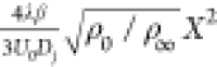 , where ρ0 and ρ∞ denote the densities
of the inlet
fuel jet and the hot-coflow, respectively. β = 0.056 is the
entrainment constant and λ equals 1.19. It can be seen that
the τres computed by eq 17 agrees well with this empirical value.
, where ρ0 and ρ∞ denote the densities
of the inlet
fuel jet and the hot-coflow, respectively. β = 0.056 is the
entrainment constant and λ equals 1.19. It can be seen that
the τres computed by eq 17 agrees well with this empirical value.
Figure 8.

Comparison of the residence time τres computed by different models.
Figure 9 shows the mass fraction and temperature profiles computed from the different TCA models as well as the reference computations of the tPDF method61 and the EDC model,19 where the multispecies transport equations were solved. Since the standard EDC overpredicted the MILD flame temperature, the predictions of an improved EDC formulation proposed by Parente et al.19 are considered for the present discussion. It can be seen that in general the FPV and PSR0 predictions are in a good agreement with the measurements and have a comparative result with the computations of tPDF and EDC models. However, FPV achieves the better predictions of radial profiles of experimental measurements. The PSR-based simulation, on the other hand, tends to underestimate the temperature and species mass fraction near the central region of jet. This could be due to the lack of the inherent structure in the PSR library that takes into account the microscale diffusive effect and its close-coupling with chemistry among the different reactive mixtures, although in the PSR reactor the nominal residence time is applied to accommodate the mixing effect induced by flow transport. The balance between molecular diffusion and chemistry is included in the flamelet equations.
Figure 9.

Comparison of temperature as well as species
mass fraction  and
and  for flames HM1 and HM3 (dots, experiments;
line, computed results from different combustion models) at axial
locations X = 30, 60 mm.
for flames HM1 and HM3 (dots, experiments;
line, computed results from different combustion models) at axial
locations X = 30, 60 mm.
The similar underestimation indicated by the PSR-based tabulation approach is also found in the PSR calculations using the chemical databases that accommodate explicitly the residence time by eq 16. It shows that the case PSRτ1 performs better than PSRτ2, but their computations are both lower than the library (PSR0) parametrized by the reaction progress variable. To explore the reason, the additional case PSRτ3 is performed which adopts a constant τres of 0.012 s that is determined by the averaging along the jet flame conditioned on the stoichiometric state of Zst. Shown in Figure 8, this constant τres is higher than other two model values, and thus this larger τres leads to a slightly improved prediction of temperature and species mass fraction (see Figures 9 and 10).
Figure 10.

Comparison of species mass fraction YCO,  , and YOH for
flames HM1 and HM3 (dots, experiments; line, computed results from
different combustion models) at axial locations X = 30, 60 mm.
, and YOH for
flames HM1 and HM3 (dots, experiments; line, computed results from
different combustion models) at axial locations X = 30, 60 mm.
The previous study showed that in the nonpremixed turbulent flame, due to the importance of the time history of the flow engulfment and micromixing processes, the accurate prediction usually needs the consideration of the mixing constraint given by both the microdiffusive effect and the turbulent-mixing acting on the fluid particles;60 these two subprocesses are commonly described by τmix and τres, respectively. Therefore, the under-predictions in cases PSRτ1, PSRτ2, and PSRτ3 may indicate that the parametrization of flow in the MILD flame with strong coupling of turbulence and chemistry needs an approach considering the multiscale mixing process.
The comparison of the minor species YCO, YOH, and  shown in Figure 10 further illustrates the performance of
the combustion models considered. FPV and PSR0 profiles are in a reasonable
agreement with the trend indicated by the experimental data. At the
same time, contrary to what is observed in flamelet prediction, a
slightly narrower distribution is noticed by the use of the PSR tabulation
approach. Particularly, it is noteworthy that the PSR0 prediction
of the YCO peak value in HM1 seems to
be lower than the FPV computations, whereas in the HM3 flame PSR0
has a higher prediction compared to FPV. This reverse trend may be
linked to the different methane oxidation processes in the MILD regime,43 which will be further explored in the next section.
shown in Figure 10 further illustrates the performance of
the combustion models considered. FPV and PSR0 profiles are in a reasonable
agreement with the trend indicated by the experimental data. At the
same time, contrary to what is observed in flamelet prediction, a
slightly narrower distribution is noticed by the use of the PSR tabulation
approach. Particularly, it is noteworthy that the PSR0 prediction
of the YCO peak value in HM1 seems to
be lower than the FPV computations, whereas in the HM3 flame PSR0
has a higher prediction compared to FPV. This reverse trend may be
linked to the different methane oxidation processes in the MILD regime,43 which will be further explored in the next section.
With the above analysis, the tabulation strategy shows its influential
role in the prediction of the MILD flame structures, and especially,
the parametrization based on the reaction progress variable outperforms
the one using τres. Figure 11 illustrates the mapping structure of PSR0
computations in the T – Z space. The PSR0 data are extracted from the flame zone with chemical
reaction rate larger than the 50% of maximum value  , corresponding to a spatial domain within
the X ≤ 60 mm. The color of scatter data represents the magnitude
of local Damköhler number that is defined as
, corresponding to a spatial domain within
the X ≤ 60 mm. The color of scatter data represents the magnitude
of local Damköhler number that is defined as  . The time
history of the PSR flame structures
in the library parametrized by τres is shown by the
solid lines. It is observed that with increasing the residence time,
the burning structure evolves from the lower mixing state to the upper
equilibrium state, and at the higher O2 levels of case
HM3, this evolving process is even faster. On the other hand, the
most chemically reactive state accessed by PSR0 prediction mainly
locates in a region with τres ≤ 0.05 s under
the present flame conditions. Further, the wide scatter distribution
in the T direction indicates that the complex flame
dynamics are difficult to be described by the single mixing scale
of τres. Meanwhile, it can also be seen that the
flame mainly burns in a fuel-rich region where the intense reaction
with high Da number is observed. This can be ascribed
to the diluted oxygen conditions.
. The time
history of the PSR flame structures
in the library parametrized by τres is shown by the
solid lines. It is observed that with increasing the residence time,
the burning structure evolves from the lower mixing state to the upper
equilibrium state, and at the higher O2 levels of case
HM3, this evolving process is even faster. On the other hand, the
most chemically reactive state accessed by PSR0 prediction mainly
locates in a region with τres ≤ 0.05 s under
the present flame conditions. Further, the wide scatter distribution
in the T direction indicates that the complex flame
dynamics are difficult to be described by the single mixing scale
of τres. Meanwhile, it can also be seen that the
flame mainly burns in a fuel-rich region where the intense reaction
with high Da number is observed. This can be ascribed
to the diluted oxygen conditions.
Figure 11.

The mapping structure of PSR0 calculation in T – Z space for flames HM1 and HM3. Solid lines, flame structure in PSR library parametrized by τres; the scatter points are colored by the magnitude of Damköhler number.
4.3. Analysis of Chemical Reaction Dynamics
The tabulated chemistry method makes the inclusion of detailed chemical scheme feasible in turbulent flame prediction, the effect of chemistry is then assessed in Figure 12, showing the predictions with the different kinetic mechanisms (discussed in section 3.2). It can be seen that the main structure of the flame temperature and species CO2 is well reproduced by the five different mechanisms. The major difference between the computations is indicated for the minor species CO mass fraction; the calculations using the DRM-22 and AramcoMech2.0 mechanisms overestimate the experimental data, and USC2.0 results in a similar profile compared to the GRI2.11 in the flame HM3 but shows an overprediction in HM1. In general, the KONNOV scheme reaches a more accurate prediction of both HM1 and HM3 flames and is superior to the reduced mechanism of DRM-22. This confirms the necessity for the use of detailed chemistry in the prediction of MILD flame. At the same time, consistent with previous findings,39 the minor species CO is found to be more sensitive to the degree of complexity in the chemical mechanism and as revealed above, to the description of turbulence/chemistry interactions.
Figure 12.

Comparison
of temperature, species mass fraction  and YCO for
flames HM1 and HM3 (dots, experiments; line, computed results with
different chemical schemes) at axial locations X =
30, 60 mm.
and YCO for
flames HM1 and HM3 (dots, experiments; line, computed results with
different chemical schemes) at axial locations X =
30, 60 mm.
As reported in refs (1 and 43), compared to the conventional combustion, the pathway of CH4 to CO/CO2 would change under the heavily diluted MILD condition. By comparing the simulations with the detailed and reduced chemical mechanisms, Aminian et al.17 attributed the discrepancies in CO prediction to the C2 chemistry, especially the oxidation of acetylene to CO. Glarborg and Bentzen62 found that the presence of high CO2 concentration has a noticeable effect on CO/CO2 interconversion, for which the dominated reaction step includes the endothermic reaction of CO2 + H ⇌ CO + OH. Meanwhile, in addition to the diluted O2 level,43 the reactor temperature and fluid residence time can also modify significantly the methane oxidation pathways to CO and CO2.15 Therefore, the different behavior of FPV and PSR0 in CO prediction for cases HM1 and HM3, as shown in Figure 10, motivates an in-depth study of methane conversion to CO/CO2 in terms of chemical reaction dynamics. To this end, a reaction pathway analysis is conducted. The chemical states that are representative of the FPV and PSR0 computations, are obtained by averaging the computed flames over the intense reaction zone, which are shown with the temperature (T) and main species in Table 3. The main pathways, in which methane is transformed to the end product CO/CO2, are then depicted in Figure 13 using the element fluxes analysis.63 The conversion between different species is described by the interconnecting arrows with the product species at the head. Each arrow representing the combined elementary reactions has a width proportional to the relative magnitude of the reaction flux θ1,i,j, which is defined as
| 18 |
where qi,j,k denotes the rate-of-production (RoP) of the kth reaction from species i to j. Three types of arrow widths are considered based on θ1,i,j values for the selected ranges shown in Figure 13. The importance of each reaction pathway is then correlated to the θ1,i,j. In addition, the exothermic and endothermic pathways are denoted by black and blue color, respectively. Here, θ2,i,j is the percentage of species i consuming specific species to produce species j, which is shown along with each arrow.
Table 3. Averaged Chemical States Computed by FPV and PSR0 in HM1 and HM3.
| HM1 |
HM3 |
|||||||||
|---|---|---|---|---|---|---|---|---|---|---|
| Model | YH2O | YCO2 | YC2H2 | YCO | T[K] | YH2O | YCO2 | YC2H2 | YCO | T[K] |
| FPV | 8.05 × 10–02 | 5.62 × 10–02 | 8.68 × 10–04 | 1.11 × 10–02 | 1414 | 1.08 × 10–01 | 6.56 × 10–02 | 7.9 × 10–04 | 2.24 × 10–02 | 1626 |
| PSR0 | 7.77 × 10–02 | 5.62 × 10–02 | 4.58 × 10–04 | 8.11 × 10–03 | 1387 | 1.08 × 10–01 | 5.89 × 10–02 | 2.37 × 10–03 | 3.09 × 10–02 | 1601 |
Figure 13.

Reaction pathways constructed based on the representative chemical structures in four computational cases. The exothermic and endothermic reactions are denoted by black and blue color, respectively, and the path width describes the relative magnitude of reaction flux.
As shown in Figure 13, the reaction progress from CH4 to CO2 is accomplished mainly through the central route, together with several side loops starting from the methyl radical CH3. In this diagram, the important intermediate species also include the CH2O and HCO, which act as the terminals for the side loops, and proceed eventually to form the end products of CO and CO2. In a comparison to the HM1 case, the chemical pathway for the HM3 case shown in Figure 13 (c) and (d) has a similar map except for the additional right-hand side loops of CH3 to C2H4 through the recombination channel (CH3 to ethane) and CH3 to CH2O through the methanol and hydroxymethyl in FPV computation. This may be due to the highest local temperature predicted in FPV-HM3 shown in Table 3, which favors the following endothermic H-abstraction reactions, CH3O(+M) ⇒ H + CH2O(+M), C2H5(+M) ⇒ H + C2H4(+M) that are accounting for around 50% contribution in the conversions of C2H5 → C2H4 and CH3O → CH2O (see Figure 13(c)).
As to the other side, the attacks on methyl radical by OH and H radicals produce the intermediate CH2(s) and subsequently the CH2 by reaction with N2 and H2O. Further, CH2 reacts with H and OH radicals to form CH which then provides three different routes to the end products of CO/CO2, i.e., (1)CH → CH2O → HCO → CO; (2)CH → HCO → CO; (3)CH → C2H4 → C2H3 → C2H2 → CO.
On the whole, FPV and
PSR0 computations of both flame cases share
similarities on the reaction pathways of methane oxidation to CO2, although the θ1,i,j and θ2,i,j differ slightly from case to case. Specifically, for CO species,
based on the order of magnitude of θ1,i,j, two main formation routes of HCO →
CO, C2H2 → CO and one consumer route
of CO → CO2 could be identified. Their absolute
rate of production (RoP) and net production rate are listed in Table 4. It can be seen that
in HM1, FPV attains a higher net production rate than PSR0 does, and
conversely in HM3, the value from FPV is lower, which explains the
reverse trend in prediction of CO mass fraction between FPV and PSR0
in two flame cases (shown in Figure 10). In addition, Table 4 also indicates that the path of C2H2 → CO or O + C2H2 ⇒ CO
+ CH2 contributes mostly to the net production rate and
therefore the different CO predictions. As shown in Table 3, this is consistent with different
values of  computed by FPV and PSR0 for two flame
cases. It is noteworthy that the pyrolytic species C2H2 is favored as one end product in a fuel-rich condition with
moderate temperature.64 Recalling the previous
observation that the reaction in HM1 and HM3 mainly burns under a
fuel-rich condition, this distinct prediction in
computed by FPV and PSR0 for two flame
cases. It is noteworthy that the pyrolytic species C2H2 is favored as one end product in a fuel-rich condition with
moderate temperature.64 Recalling the previous
observation that the reaction in HM1 and HM3 mainly burns under a
fuel-rich condition, this distinct prediction in  and YCO reflects
the different model performance.
and YCO reflects
the different model performance.
Table 4. Rate-of-Production of Three Reaction Routes for FPV and PSR0 Computations of HM1 and HM3. RoP Has a Unit of g mol/cm3 s.
| HM1 |
HM3 |
|||
|---|---|---|---|---|
| Reaction path | FPV/RoP | PSR0/RoP | FPV/RoP | PSR0/RoP |
| HCO → CO | 1.895 × 10–05 | 2.124 × 10–05 | 5.345 × 10–04 | 3.713 × 10–04 |
| C2H2 → CO | 3.195 × 10–05 | 2.214 × 10–05 | 2.107 × 10–04 | 7.235 × 10–04 |
| CO → CO2 | –4.266 × 10–05 | –4.144 × 10–05 | –3.968 × 10–04 | –6.522 × 10–04 |
| Net | 0.824 × 10–05 | 0.194 × 10–05 | 3.484 × 10–04 | 4.426 × 10–04 |
This finding implies that in the MILD flame of HM1 that is prone to well-mixed (see Figure 4), compared to PSR, the tabulation approach FPV assuming a thin flame front might overestimate the intensity of the reaction region, while in the flame HM3 that deviates from the MILD condition where the thin reaction zone interacted over a large range of mixing scale, FPV considering the microscale diffusion/chemistry competition outperforms the PSR-based modeling.
As shown in ref (34), under the hot diluted condition, flame may still be characterized by a transition in combustion regimes, where apart from the MILD zone, the Quasi-MILD and MILD-like combustion could be observed. Therefore, the implication given above necessitates the use of multiregime combustion models for the accurate prediction of MILD combustion, particularly when more complex turbulent flowfield/chemistry interactions involved in various industrial burners are considered.
5. Conclusions
In the present work, the tabulated chemistry approach (TCA) for MILD combustion modeling was thoroughly assessed in the context of RANS simulations of Adelaide JHC burner. The sensitivities to the submodel accouting for the micromixing of passive and reactive scalars, and the tabulation strategy (by use of the Flamelet and PSR reactors) were analyzed. The impact of chemical kinetics with different detailed mechanisms and the implication of variations in the primary kinetic pathways at different flame conditions were also discussed. The main conclusions are drawn as follows,
The
 can be determined by the lifetime of mechanical
turbulence, the same as the passive scalar of mixture fraction, and
the more complex algebraic closure of
can be determined by the lifetime of mechanical
turbulence, the same as the passive scalar of mixture fraction, and
the more complex algebraic closure of  does not guarantee a further improvement
since the current flames appear to be a typical fuel/oxidant mixing-dominated
flame.
does not guarantee a further improvement
since the current flames appear to be a typical fuel/oxidant mixing-dominated
flame.The chemical effect was discussed employing five different chemical schemes. In general, except for the AramcoMech2.0, the detailed mechanisms performed better in the prediction of both major and minor species (e.g., CO). The KONNOV mechanism attained a slightly more accurate result.
Overall, the TCA with a proper modeling of micromixing, can well reproduce the MILD flame structures, and also showed a comparable prediction capability but far less computational cost in a comparison to the transported PDF method and EDC model.
By means of the kinetic pathway analysis, the endothermic reaction path of O + C2H2 ⇒ CO + CH2 was identified as the main contributing cause to the difference in CO predictions obtained by flamelet and PSR calculations. The results highlighted the influential role of the multiscale mixing process and its competitions with chemistry, accurate closure of which was important for MILD combustion modeling.
Acknowledgments
This research has received funding support from the National Natural Science Foundation of China (Grant No. 52006151,52006152), National Key R&D Program of China (Grant No. 2022YFC3003100), and “the Fundamental Research Funds for the Central Universities” under the Projects (YJ201943, YJ202019).
Glossary
Nomenclature
- α
mass diffusivity, m2/s
- χΦ
dissipation rate of scalar Φ, 1/s
- μt
turbulent viscosity, kg/m/s
- ν
kinematic viscosity, m2/s

stress tensor, N/m2

turbulent kinetic energy dissipation rate, m2/s3

turbulent kinetic energy, m2/s2

gas velocity, m/s

reaction source term of progress variable, 1/s

variance of progress variable, -

mixture fraction, -

variance of mixture fraction, -
- Dj
jet nozzle diameter, m

laminar flame speed, m/s
- Sct
Schmidt number, -
- Zst
stoichiometric mixture fraction, -
- ρ
gas density, kg/m3
- ρu
unburnt mixture density, kg/m3
- τres
residence time, s
- τmix
turbulent mixing time, s
- p
pressure, Pa
- T
gas temperature, K
The authors declare no competing financial interest.
References
- Cavaliere A.; de Joannon M. MILD combustion. Proc. Combust. Inst. 2004, 30, 329–66. 10.1016/j.pecs.2004.02.003. [DOI] [Google Scholar]
- Weber R.; Smart J. P.; Kamp W. On the (MILD) combustion of gaseous, liquid, and solid fuels in high temperature preheated air. Prog. Energy Combust. 2005, 30, 2623–2629. 10.1016/j.proci.2004.08.101. [DOI] [Google Scholar]
- Wünning J. A.; Wünning J. G. Flameless oxidation to reduce thermal no formation. Prog. Energy Combust. 1997, 23, 81–94. 10.1016/S0360-1285(97)00006-3. [DOI] [Google Scholar]
- Zornek T.; Monz T.; Aigner M. Performance analysis of the micro gas turbine Turbec T100 with a new FLOX-combustion system for low calorific fuels. Appl. Energy 2015, 159, 276–284. 10.1016/j.apenergy.2015.08.075. [DOI] [Google Scholar]
- Saha M.; Chinnici A.; Dally B. B.; Medwell P. R. Numerical study of pulverized coal MILD combustion in a self-recuperative furnace. Energy Fuels 2015, 29, 7650–7669. 10.1021/acs.energyfuels.5b01644. [DOI] [Google Scholar]
- Dally B. B.; Karpetis A. N.; Barlow R. S. Structure of turbulent non-premixed jet flames in a diluted hot coflow. Proc. Combust. Inst. 2002, 29, 1147–1154. 10.1016/S1540-7489(02)80145-6. [DOI] [Google Scholar]
- Evans M. J.; Medwell P. R.; Tian Z. F.; Ye J.; Frassoldati A.; Cuoci A. Effects of oxidant stream composition on non-premixed laminar flames with heated and diluted coflows. Combust. Flame 2017, 178, 297–310. 10.1016/j.combustflame.2016.12.023. [DOI] [Google Scholar]
- Ye J.; Medwell P. R.; Evans M. J.; Dally B. B.. The impact of carrier gas on ethanol flame behaviour in a Jet in Hot Coflow (JHC) burner. Proceedings of the Australian Combustion Symposium, Melbourne Australia, December 7–9, 2015.
- Plessing T.; Peters N.; Wünning J. Laseroptical Investigation of highly preheated combustion with strong exhaust gas recirculation. Symp. (Int.) Combust. 1998, 27, 3197–3204. 10.1016/S0082-0784(98)80183-5. [DOI] [Google Scholar]
- Szegö G. G.; Dally B. B.; Nathan G. J. Operational characteristics of a parallel jet MILD combustion burner system. Combust. Flame 2009, 156, 429–438. 10.1016/j.combustflame.2008.08.009. [DOI] [Google Scholar]
- Derudi M.; Villani A.; Rota R. Sustainability of mild combustion of hydrogen-containing hybrid fuels. Proc. Combust. Inst. 2007, 31, 3393–3400. 10.1016/j.proci.2006.08.107. [DOI] [Google Scholar]
- Li P.; Dally B. B.; Mi J.; Wang F. MILD oxy-combustion of gaseous fuels in a laboratory-scale furnace. Combust. Flame 2013, 160, 933–946. 10.1016/j.combustflame.2013.01.024. [DOI] [Google Scholar]
- Li P.; Wang F.; Mi J.; Dally B. B.; Mei Z. MILD Combustion under Different Premixing Patterns and Characteristics of the Reaction Regime. Energy Fuels 2014, 28, 2211–2226. 10.1021/ef402357t. [DOI] [Google Scholar]
- Ertesvåg I. S. Analysis of Some Recently Proposed Modifications to the Eddy Dissipation Concept(EDC). Combust. Sci. Technol. 2020, 192, 1108–1136. 10.1080/00102202.2019.1611565. [DOI] [Google Scholar]
- Mardani A. Optimization of the Eddy Dissipation Concept (EDC) model for turbulence-chemistry interactions under hot diluted combustion of CH4/H2. Fuel 2017, 191, 114–129. 10.1016/j.fuel.2016.11.056. [DOI] [Google Scholar]
- De A.; Oldenhof E.; Sathiah P.; Roekaerts D. Numerical simulation of Delft-Jet-in-Hot-Coflow (DJHC) flames using the eddy dissipation concept model for turbulence-chemistry interaction. Flow Turbul. Combust. 2011, 87, 537–567. 10.1007/s10494-011-9337-0. [DOI] [Google Scholar]
- Aminian J.; Galletti C.; Shahhosseini S.; Tognotti L. Numerical Investigation of a MILD Combustion Burner: Analysis of Mixing Field, Chemical Kinetics and Turbulence-Chemistry Interaction. Flow Turbul. Combust. 2012, 88, 597–623. 10.1007/s10494-012-9386-z. [DOI] [Google Scholar]
- Evans M. J.; Medwell P. R.; Tian Z. F. Modelling Lifted Jet Flames in a Heated Coflow using an Optimised Eddy Dissipation Concept Model. Combust. Sci. Technol. 2015, 187, 1093–1109. 10.1080/00102202.2014.1002836. [DOI] [Google Scholar]
- Parente A.; Malik M. R.; Contino F.; Cuoci A.; Dally B. B. Extension of the Eddy Dissipation Concept for turbulence/chemistry interactions to MILD combustion. Fuel 2016, 163, 98–111. 10.1016/j.fuel.2015.09.020. [DOI] [Google Scholar]
- Christo F. C.; Dally B. B.. Application of Transport PDF Approach for Modelling MILD Combustion. 15th Australasian Fluid Mechanics Conference. Sydney, Australia, December, 2004.
- Ma L.; Roekaerts D. Structure of Spray in Hot-Diluted Coflow Flames Under Different Coflow Conditions: A Numerical Study. Combust. Flame 2016, 172, 20–37. 10.1016/j.combustflame.2016.06.017. [DOI] [Google Scholar]
- Peters N.Turbulent Combustion; Cambridge University Press: Cambridge, 2000. [Google Scholar]
- Fiorina B.; Gicquel O.; Vervisch L.; Carpentier S.; Darabiha N. Approximating the chemical structure of partially premixed and diffusion counterflow flames using FPI flamelet tabulation. Combust. Flame 2005, 140, 147–160. 10.1016/j.combustflame.2004.11.002. [DOI] [Google Scholar]
- Wen J.; Hu Y.; Nishiie T.; Iino J.; Masri A.; Kurose R. A flamelet LES of turbulent dense spray flame using a detailed high-resolution VOF simulation of liquid fuel atomizatione. Combust. Flame 2021, 28, 111742. 10.1016/j.combustflame.2021.111742. [DOI] [Google Scholar]
- Hu Y.; Kurose R. Nonpremixed and premixed flamelets LES of partially premixed spray flames using a two-phase transport equation of progress variable. Combust. Flame 2018, 188, 227–42. 10.1016/j.combustflame.2017.10.004. [DOI] [Google Scholar]
- Ihme M.; See Y. C. LES flamelet modeling of a three-stream MILD combustor: Analysis of flame sensitivity to scalar inflow conditions. Proc. Combust. Inst. 2011, 33, 1309–1317. 10.1016/j.proci.2010.05.019. [DOI] [Google Scholar]
- Lamouroux J.; Ihme M.; Fiorina B.; Gicquel O. Tabulated chemistry approach for diluted combustion regimes with internal recirculation and heat losses. Combust. Flame 2014, 161, 2120–2136. 10.1016/j.combustflame.2014.01.015. [DOI] [Google Scholar]
- Abtahizadeh E.; de Goey P.; van Oijen J. Development of a novel flamelet-based model to include preferential diffusion effects in autoignition of CH4/H2 flame. Combust. Flame 2015, 162, 4358–4369. 10.1016/j.combustflame.2015.06.015. [DOI] [Google Scholar]
- Sidey J.; Mastorakos E. Visualization of MILD combustion from jets in cross-flow. Proc. Combust. Inst. 2015, 35, 3537–3545. 10.1016/j.proci.2014.07.028. [DOI] [Google Scholar]
- Minamoto Y.; Swaminathan N.; Cant S. R.; Leung T. Morphological and statistical features of reaction zones in MILD and premixed combustion. Combust. Flame 2014, 161, 2801–2814. 10.1016/j.combustflame.2014.04.018. [DOI] [Google Scholar]
- Chen Z.; Reddy V. M.; Ruan S.; Doan N. A. K.; Roberts W. L.; Swaminathan N. Simulation of MILD combustion using perfectly stirred reactor model. Proc. Combust. Inst. 2017, 36, 4279–4286. 10.1016/j.proci.2016.06.007. [DOI] [Google Scholar]
- Chitgarha F.; Mardani A. Assessment of steady and unsteady flamelet models for MILD combustion modeling. Int. J. Hydrogen Energy 2018, 43, 15551–15563. 10.1016/j.ijhydene.2018.06.071. [DOI] [Google Scholar]
- Hu Y.; Kurose R. Large-eddy simulation of turbulent autoigniting hydrogen lifted jet flame with a multi-regime flamelet approach. Int. J. Hydrogen Energy 2019, 44, 6313–6324. 10.1016/j.ijhydene.2019.01.096. [DOI] [Google Scholar]
- Wang F.; Li P.; Mei Z.; Zhang J.; Mi J. Combustion of CH4/O2/N2 in a well stirred reactor. Energy 2014, 72, 242–253. 10.1016/j.energy.2014.05.029. [DOI] [Google Scholar]
- Pope S. B. PDF methods for turbulent reactive flows. Prog. Energy Combust. Sci. 1985, 11, 119–192. 10.1016/0360-1285(85)90002-4. [DOI] [Google Scholar]
- Hu Y.; Olguin H.; Gutheil E. Transported joint probability density function simulation of turbulent spray flames combined with a spray flamelet model using a transported scalar dissipation rate. Combust. Sci. Technol. 2017, 189, 322–39. 10.1080/00102202.2016.1214584. [DOI] [Google Scholar]
- Cao R. R.; Wang H.; Pope S. B. The effect of mixing models in PDF calculations of piloted jet flames. Proc. Combust. Inst. 2007, 31, 1543–1550. 10.1016/j.proci.2006.08.052. [DOI] [Google Scholar]
- Magnussen B. F. On the structure of turbulence and a generalized eddy dissipation concept for chemical reaction in turbulent flow. Proc. 19th AIAA Aerospace Meet. 1981, A81.37570 10.2514/6.1981-42. [DOI] [Google Scholar]
- Li Z.; Cuoci A.; Sadiki A.; Parente A. Comprehensive numerical study of the Adelaide Jet in Hot-Coflow burner by means of RANS and detailed chemistry. Energy 2017, 139, 555–570. 10.1016/j.energy.2017.07.132. [DOI] [Google Scholar]
- Golovitchev V.; Tretjalpv P.; Raffoul C. Evaluation of Drag Reduction of Blunt Bodies at Supersonic Speeds by Counter-flow Combustion. Proc. 32nd AIAA Fluid Dynamic Conf. 2002, 1–14. 10.2514/6.2002-3296. [DOI] [Google Scholar]
- Ihme M.; See Y. C. Prediction of autoignition in a lifted methane/air flame using an unsteady flamelet/progress variable model. Combust. Flame 2010, 157, 1850–1862. 10.1016/j.combustflame.2010.07.015. [DOI] [Google Scholar]
- Kuan T. S.; Lindstedt R. P.; Vaos E. M.. Higher moment based modeling of turbulence enhanced explosion kernels in confined fuel-air mixtures, In Advances in Confined Detonations and Pulse Detonation Engines; Torus Press: Moscow, 2003; pp 17–40. [Google Scholar]
- Christo F. C.; Dally B. B. Modeling turbulent reacting jets issuing into a hot and diluted coflow. Combust. Flame 2005, 142, 117–129. 10.1016/j.combustflame.2005.03.002. [DOI] [Google Scholar]
- Fluent 13.0 UDF Manual; ANSYS, 2010.
- Mardani A.; Tabejamaat S.; Hassanpour S. Numerical study of CO and CO2 formation in CH4/H2 blended flame under MILD condition. Combust. Flame 2013, 160, 1636–1649. 10.1016/j.combustflame.2013.04.003. [DOI] [Google Scholar]
- Wang F.; Mi J.; Li P.; Zheng C. Diffusion flame of a CH4/H2 jet in hot low-oxygen coflow. Int. J. Hydrogen Energy 2011, 36, 9267–9277. 10.1016/j.ijhydene.2011.04.180. [DOI] [Google Scholar]
- Kazakov A.; Frenklach M.. Reduced reaction sets based on GRI-Mech 1.2. http://combustion.berkeley.edu/drm/ (accessed 2023).
- Bowman C. T.; Hanson R. K.; Davidson D. F.; Gardiner W. C.; Lissianski V.; Smith G. P.; Golden D. M.; Frenklach. GRI-Mech 2.11, ver. 2.11; Berkeley: www.me.berkeley.edu/gri-mech/.
- Wang H.; You X. Q.; Joshi A. V.; Davis S. G.; Laskin A.; Egolfopoulos F.; Law C. K.. USC Mech Version II. High-Temperature Combustion Reaction Model of H2/CO/C1-C4 Compounds, http://ignis.usc.edu/USC_Mech_II.htm, 2007.
- The following citation is often used but does not exist anymore: A. A. Konnov. Detailed reaction mechanism for small hydrocarbons combustion. Release 0.5. http://homepages.vub.ac.be/akonnov/, 2000. Recommended citation (Chemkin files in the supplementary materials):Coppens F. H. V.; De Ruych J.; Konnov A. A. The effects of composition on burning velocity and nitric oxide formation in laminar premixed flames of CH4 + H2 + O2 + N2. Combust. Flame 2007, 149, 409. 10.1016/j.combustflame.2007.02.004. [DOI] [Google Scholar]
- Li Y.; Zhou C. W.; Somers K. P.; Zhang K.; Curran H. J. The oxidation of 2-butene: a high pressure ignition delay, kinetic modeling study and reactivity comparison with isobutene and 1-butene. Proc. Combust. Inst. 2017, 36, 403–411. 10.1016/j.proci.2016.05.052. [DOI] [Google Scholar]
- Pitsch H.FlameMaster v3.1: A C++ Computer Program for 0D Combustion and 1D Laminar Flame Calculations; H. Pitsch, 1998.
- Glarborg P.; Kee R. J.; Grcar J. F.; Miller J. A.. PSR. A Fortran Program for Modeling Well-Stirred Reactors; DTU, 1986; No. SAND86-8209.
- Mastorakos E.; Taylor A. M. K. P.; Whitelaw J. H. Extinction of turbulent counterflow flames with reactants diluted by hot products. Combust. Flame 1995, 102, 101–114. 10.1016/0010-2180(94)00252-N. [DOI] [Google Scholar]
- Shu Z.; Dai C.; Li P.; Mi J. Nitric oxide of MILD combustion of a methane jet flame in hot oxidizer coflow: Its formations and emissions under H2O, CO2 and N2 dilutions. Fuel 2018, 234, 567–580. 10.1016/j.fuel.2018.07.057. [DOI] [Google Scholar]
- Tu Y.; Liu H.; Yang W. Flame Characteristics of CH4/H2 on a Jet-in-Hot-Coflow Burner Diluted by N2, CO2, and H2O. Energy Fuels 2017, 31, 3270–3280. 10.1021/acs.energyfuels.6b03246. [DOI] [Google Scholar]
- Duwig C.; Li B.; Li Z. S.; Aldén M. High resolution imaging of flameless and distributed turbulent combustion. Combust. Flame 2012, 159, 306–316. 10.1016/j.combustflame.2011.06.018. [DOI] [Google Scholar]
- Özdemir iB.; Peters N. Characteristics of the reaction zone in a combustor operating at mild combustion. Exp. Fluids 2001, 30, 683–695. 10.1007/s003480000248. [DOI] [Google Scholar]
- Hu I.; Correa S. M. Calculations of turbulent flames using a PSR microstructural library. Symp. (Int.) Combust. 1996, 26, 307–313. 10.1016/S0082-0784(96)80230-X. [DOI] [Google Scholar]
- Enjalbert N.; Domingo P.; Vervisch L. Mixing time-history effects in Large Eddy Simulation of non-premixed turbulent flames: Flow-Controlled Chemistry Tabulation. Combust. Flame 2012, 159, 336–352. 10.1016/j.combustflame.2011.06.005. [DOI] [Google Scholar]
- Lee J.; Jeon S.; Kim Y. Multi-environment probability density function approach for turbulent CH4/H2 flames under the MILD combustion condition. Combust. Flame 2015, 162, 1464–1476. 10.1016/j.combustflame.2014.11.014. [DOI] [Google Scholar]
- Glarborg P.; Bentzen L. B. Chemical Effects of a High CO 2 Concentration in Oxy-Fuel Combustion of Methane. Energy Fuels 2008, 22, 291–296. 10.1021/ef7005854. [DOI] [Google Scholar]
- Revel J.; Boettner J. C.; Cathonnet M.; Bachman J. S. Derivation of a global chemical kinetic mechanism for methane ignition and combustion. J. Chem. Phys. 1994, 91, 365–382. 10.1051/jcp/1994910365. [DOI] [Google Scholar]
- de Joannon M.; Saponaro A.; Cavaliere A. Zero-dimensional analysis of diluted oxidation of methane in rich conditions. Proc. Combust. Inst. 2000, 28, 1639–1646. 10.1016/S0082-0784(00)80562-7. [DOI] [Google Scholar]