Protocol for using serial two-photon tomography to map cell types and cerebrovasculature at single-cell resolution in the whole adult mouse brain

Summary

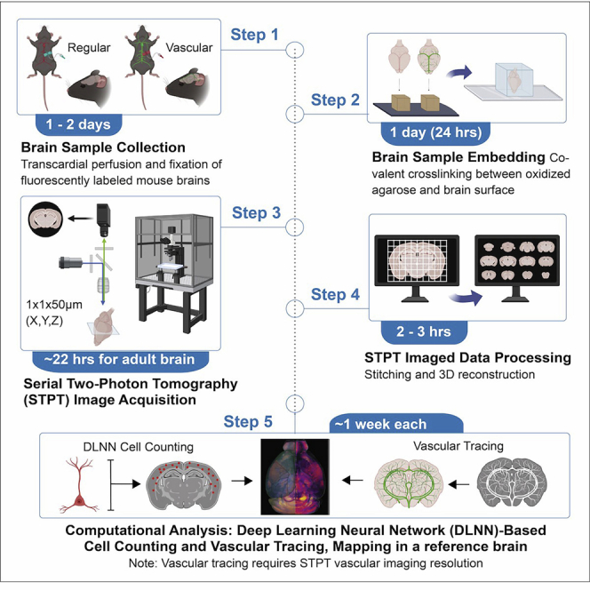
Here, we present a protocol using serial two-photon tomography (STPT) to quantitatively map genetically defined cell types and cerebrovasculature at single-cell resolution across the entire adult mouse brain. We describe the preparation of brain tissue and sample embedding for cell type and vascular STPT imaging and image processing using MATLAB codes. We detail the computational analyses for cell signal detection, vascular tracing, and three-dimensional image registration to anatomical atlases, which can be implemented for brain-wide mapping of different cell types.

For complete details on the use and execution of this protocol, please refer to Wu et al. (2022),¹ Son et al. (2022),² Newmaster et al. (2020),³ Kim et al. (2017),⁴ and Ragan et al. (2012).⁵

Graphical abstract

Highlights

• •A protocol to use serial two-photon tomography (STPT) for whole mouse brain imaging
• •Steps for brain sample collection and embedding for STPT imaging
• •Computational analysis pipelines for quantitative cell type and cerebrovascular mapping
• •Can be applied for brain-wide mapping of different cell types

Publisher’s note: Undertaking any experimental protocol requires adherence to local institutional guidelines for laboratory safety and ethics.

Here, we present a protocol using serial two-photon tomography (STPT) to quantitatively map genetically defined cell types and cerebrovasculature at single-cell resolution across the entire adult mouse brain. We describe the preparation of brain tissue and sample embedding for cell type and vascular STPT imaging and image processing using MATLAB codes. We detail the computational analyses for cell signal detection, vascular tracing, and three-dimensional image registration to anatomical atlases, which can be implemented for brain-wide mapping of different cell types.

Before you begin

In this detailed protocol, we describe a microscopy imaging and computational analysis pipeline to perform high-resolution mapping of genetically labeled cell types and the cerebrovasculature in the adult mouse brain. By utilizing serial two-photon tomography (STPT), we are poised to perform cellular resolution imaging followed by quantitative assessment of cell types and vascular components across the entire mouse brain.

Previously, we developed and applied this pipeline to study the stereotypical distributions of several inhibitory cell types, including somatostatin-positive, parvalbumin-positive, and vasoactive intestinal peptide-positive neurons in the adult mouse brain, since these GABAergic subtypes comprise a large majority of brain cell types and are heavily implicated in neurological diseases.⁴ We then utilized this platform to quantitatively map oxytocin receptor-expressing cells in the postnatally developing mouse brain, as oxytocin receptor-mediated signaling of oxytocin plays a critical role in the development of animal social behavior, among other critical developmental functions.³ Most recently, we evaluated the spatial relationships between the cerebrovascular network and different neuronal cell types in isocortical and largely understudied subcortical areas of the adult mouse brain, since many cell types are energy-demanding and are involved in neurovascular coupling for normal brain health and function.¹

For users interested in studying the whole-brain architecture of other cell types or the cerebrovasculature, this resource provides opportunities for quantitatively assessing their spatial relationships across different regions of the mouse brain.

This protocol includes a complete list of materials and equipment required, which are all listed in the key resources table. Solutions are prepared following the instructions in this before you begin section, in addition to the recipes found in the materials and equipment section. Solutions that can be prepared in advance and stored are indicated.

Institutional permissions

All experiments and techniques involving live animals have been approved and conform to the regulatory standards set by the Institutional Animal Care and Use Committee (IACUC) at Pennsylvania State University. Please be sure to acquire the appropriate permissions from relevant institutions before performing any experiments described in this protocol or elsewhere.

Preparation of oxidized agarose

Timing: 4 h (for steps 1 to 9)

This section outlines the steps required to prepare a solution of oxidized agarose for STPT Brain sample embedding. Please refer to the key resources table and materials and equipment section for necessary reagents and related recipe.

• 1.Oxidized agarose is light-sensitive. Before preparing this reagent, make sure to completely cover the glassware being used in aluminum foil.

CRITICAL: The glass beaker must stay protected from light for the entire duration of the preparation process.

Note: It is recommended to use a 600 mL Pyrex beaker made of borosilicate glass.

• 2.
  Pour 350 mL of 0.05 M phosphate buffer (PB) into the glass beaker with a magnetic stir bar.

  • a.
    Place the beaker on a stirring hot plate and set the stir setting to 400 RPM, but do not turn on the heat setting.
  • b.
    Ensure the beaker and the stirring hot plate are placed inside of a chemical fume hood for the duration of the protocol.
• 3.Weigh out 7 g of agarose (Fisher Scientific, BP1356-100) and slowly add to the already-stirring PB in the glass beaker.
• 4.
  Weigh out 0.74 g of sodium periodate (NaIO₄; Thermo Fisher Scientific, 198381000) and then add to stirring mixture.

  • a.
    Cover the top of the beaker with aluminum foil to protect from light, but do not seal on the sides.
• 5.Let the agarose and sodium periodate mixture in PB stir for a minimum of 2 to a maximum of 3 h.

CRITICAL: If the mixture has stirred for 4 h or more, it is highly recommended to restart the protocol with new chemical reagents.

• 6.After the 2- to 3-h time elapses, use a 1 L Pyrex media storage bottle and screw on a bottle-top vacuum filter without a stopper.
• 7.
  Connect the filter nozzle to an air vacuum source with tubing for vacuum filtration.

  • a.
    Filter the oxidized agarose 3 times with 400 mL of double-distilled water (ddH₂O).
  • b.
    Then, filter the oxidized agarose once with 400 mL of 0.05 M PB.
• 8.Fill five 50 mL conical tubes with 35 mL of 0.05 M PB.
• 9.
  Scrape out the oxidized agarose from the vacuum filter into a large weigh boat and measure the total weight in grams.

  • a.
    Record the total weight, which should approximately be 40 g.
  • b.
    Divide the total weight by 5 to obtain the amount of oxidized agarose that should be placed into each 50 mL conical tube filled with PB.

    • i.
      The final amount of oxidized agarose per tube should be around 8 g.
  • c.
    Aliquot the final amount of oxidized agarose into each vial of PB with a spatula.

Note: The easiest way to measure is to have a calculator with the total weight (g) of oxidized agarose, and then subtract the final amount obtained in step 9a from the total so that it matches the reading on the scale. Repeat this process until all 5 conical tubes are filled.

CRITICAL: For storage, all vials containing oxidized agarose suspended in 0.05 M PB must be shielded from light (i.e., wrapping the vials in aluminum foil) and kept at 4°C until use.

Pause point: Freshly prepared oxidized agarose can be stored at 4°C for 2–3 weeks.

Preparation of 0.05 M sodium borate buffer

Timing: 15 min (for steps 10 to 13)

This section outlines the steps required to prepare a solution of 0.05 M sodium borate buffer for STPT Brain sample embedding. Please refer to the key resources table and materials and equipment section for necessary reagents and related recipe.

• 10.To prepare a stock solution of sodium borate buffer (SBB, pH = 9.0–9.5), add 1 L of distilled water to a 1 L borosilicate glass beaker with a magnetic stir bar.
• 11.Place the beaker of water on a stirring hot plate and set the stirrer to 400 RPM.
• 12.Measure 19 g of sodium tetraborate decahydrate (Na₂B₄O₇·10H₂O; Honeywell Fluka, 31457) and 3 g of boric acid (H₃BO₃; Sigma-Aldrich, B0394) using weigh boats and dissolve the reagents in water via rotation-mixing for 10 min.
• 13.Move the SBB to a media storage glass bottle with screw cap for storage.

Pause point: Once prepared, SBB can be kept at 20°C–22°C for 4 weeks.

Preparation of 0.05 M sodium borohydrate buffer

Timing: 10 min (for steps 14 to 21)

This section outlines the steps required to prepare a solution of 0.05 M sodium borohydrate buffer for STPT Brain sample embedding. Please refer to the key resources table and materials and equipment section for necessary reagents and related recipe.

• 14.To prepare the sodium borohydrate buffer, pour 100 mL of SBB into a 250 mL glass bottle with screw cap.
• 15.
  Weigh out 0.2 g of sodium borohydride (NaBH₄; Sigma-Aldrich, 452882-25G).

  • a.
    Then, move the measured sodium borohydride inside of a chemical fume hood.
• 16.
  Heat the 100 mL of SBB for 15–20 s in the microwave until its temperature reaches around 40°C.

  • a.
    While the buffer is heating, create an aluminum foil cover for the 250 mL glass bottle.
  • b.
    After the elapsed time in the microwave, take the SBB out and completely wrap the bottle in the aluminum foil.
• 17.
  Quickly move the heated SSB to a chemical fume hood and place it on a stirring hot plate.

  • a.
    Use a magnetic stir bar to the bottle and set the stir setting to 300 RPM.
• 18.
  Add the measured 0.2 g of sodium borohydride to the SBB to form sodium borohydrate.

  • a.
    To make sure there is no sodium borohydride powder leftover, scoop everything out with a spatula and dunk the spatula into the stirring SBB.
• 19.Let the sodium borohydrate solution mix well for 5 min, completely shielded from light.
• 20.
  After 5 min, turn off the stir setting of the stirring hot plate and loosely screw the cap on the bottle, to the first line from the top.

  • a.
    Then, leave in the chemical fume hood overnight.

CRITICAL: This is a thermogenic reaction with gas production. Doing this procedure in a tightly sealed container can lead to an explosion.

• 21.The next morning, securely tighten the cap on the bottle.

Note: At this point, the sodium borohydrate can be used for crosslinking in the brain embedding process.

CRITICAL: Only use the solution the next day after it is prepared.

CRITICAL: A freshly made solution of sodium borohydrate can be used for up to 5 days. It is not recommended to embed tissue samples using solutions that are more than 5 days old. If STPT imaging is occurring more frequently, prepare a second bottle of sodium borohydrate on the fourth day of previously made sodium borohydrate. Discard all used solutions as hazardous solutions.

Note: Sodium borohydride is a powder that absorbs oxygen. Upon exposure to air, the texture of the powder may begin to change. Make sure to seal the container of sodium borohydride tightly with Parafilm and store in a flammable storage cabinet.

Preparation of magnetic glass slides for STPT sample setup

Timing: 20 min for preparation, 24 h for curing adhesive (for steps 22 to 31)

This section outlines the steps necessary for utilizing standard microscope slides as a tool for adhering and positioning embedded brain samples for STPT imaging, related to steps 70–73 in the following section: serial two-photon tomography (STPT) sample setup and image acquisition. Please refer to the key resources table for necessary components.

• 22.Lay down paper towels on a flat bench surface to protect from any spilled resin glue.
• 23.Take a microscope glass slide with a frosted tab and turn it over so that the textured, frosted side is facing downward, and the smooth glass side is facing up.

Note: It is recommended to prepare multiple magnetic glass slides at once to have an available stock ready in case one breaks or if the glue/magnet comes off.

• 24.
  Place two neodymium magnets (10 × 4 × 2 mm, each) apart from each other on the bottom, frosted surface of the glass slide so that the slide is on top of the magnets.

  • a.
    See Figure 1A for visualized estimate of distance between magnets on slide.
  • b.
    Since these magnets are very strong, place them far enough from each other such that they do not magnetically attract.
• 25.Place two more of the same type of magnet on the top, smooth surface of the glass slide so that they are magnetically attracted to the two magnets below the slide.

Note: This ensures that the magnets will not move from their position during adhesion.

• 26.
  Repeat steps 25 and 26 for each glass slide being prepared.

  • a.
    Make sure to leave enough space between all the glass slides.
• 27.
  Apply a two-part epoxy resin and hardener adhesive (Gorilla Glue, 4200130) to glue the magnets to the upward-facing, smooth surface of the glass slide.

  • a.
    Slowly dispense even amounts of epoxy resin and hardener onto a clean, disposable, contained surface.
  • b.
    Mix the two parts for about 15–20 s until the mixture is uniform.
  • c.
    After mixing is complete, carefully apply the epoxy-hardener adhesive around each magnet using a small wooden stick from cotton swab or a disposable spatula.

    • i.
      This should be done for all glass slides within 5 min as the epoxy will continue to thicken and the bond strength will decrease the longer you wait to apply.

Note: If there are numerous magnetic slides to prepare (more than 6), it is recommended to mix enough epoxy for 6 slides. Then, repeat step 28 for the next batch of 6 slides.

• 28.Let the epoxy mixture cure for 24 h undisturbed so that the final bond strength of the adhesive is achieved.
• 29.Once completely cured, remove the magnets not adhered to the glass slides by epoxy resin and save them for future use.
• 30.Use rough sandpaper with a coarse grit (40–50 grit range) to create scratches on the middle surface of the glass slide without magnets.

CRITICAL: This step is essential for the embedded samples to remain glued on the glass slide for extended hours in buffered solution during image acquisition.

• 31.The magnetic glass slides are now ready to be used for gluing the embedded sample-agarose blocks for STPT imaging (Figures 1A–1C).

Figure 1.

Custom STPT sample holder using a magnetic microscope glass slide

(A) Preparation of magnetic sample holders for STPT utilizes microscope glass slides. Two small neodymium magnets are adhered to the back of the glass slide using a two-part epoxy and resin mixture and left to cure for at least 24 h before using. Embedded and cross-linked brain samples are glued to a roughened top surface of the glass slide using super-strength glue (i.e., Krazy Glue).

(B) Once an embedded sample is glued to a magnetic glass slide, it can be placed inside of the STPT sample buffer chamber, which has a metal disc at the bottom to hold the glass slide in place.

(C) Depiction of mouse brain orientation (anterior end with olfactory bulbs facing down, posterior end with brainstem facing up) when gluing the embedded sample to the glass slide.

Key resources table

REAGENT or RESOURCE	SOURCE	IDENTIFIER
Chemicals, peptides, and recombinant proteins
Fluorescein isothiocyanate (FITC) conjugated albumin	Sigma-Aldrich	A9771-1G; MDL: MFCD00282182
Porcine skin gelatin	Sigma-Aldrich	G1890-500G; CAS: 9000-70-8
Ketamine (KetaVed)	Vedco	NDC: 50989-996-06
Xylazine (AnaSed)	Akorn	NDC: 59399-110-20
Paraformaldehyde, granular	Electron Microscopy Sciences	Cat#19210
Sodium hydroxide, pellets, ≥ 97.0%	Sigma-Aldrich	221465-500G; CAS: 1310-73-2
Hydrochloric acid solution, 1.0N, bioreagent, suitable for cell culture	Sigma-Aldrich	H9892-100ML; CAS: 7647-01-0
Agarose	Sigma-Aldrich	BP1356-100; CAS: 56-40-6
Sodium azide, ≥ 99.5%	Sigma-Aldrich	S2002-100G; CAS: 26628-22-8
Sodium periodate, 99% for analysis	Thermo Fisher Scientific	198381000; CAS: 7790-28-5
Sodium phosphate, monobasic	DOT Scientific	DSS23120-500; CAS: 10049-21-5
Sodium phosphate, dibasic anhydrous	DOT Scientific	DSS23100-1000; CAS: 7558-79-4
Sodium borohydride, powder, ≥ 98.0%	Sigma-Aldrich	452882-25G; CAS: 16940-66-2
Sodium tetraborate decahydrate	Honeywell/Fluke	31457-500G; CAS: 1303-96-4
Boric acid	Sigma-Aldrich	B0394-500G; CAS: 10043-35-3
Experimental models: Organisms/strains
C57BL/6J mice Age: Postnatal day 67; Sex: Male and female	Jackson Laboratory	Strain #: 000664; RRID:IMSR_JAX: 000664
nNOS-CreER (B6;129S-Nos1tm1.1(cre/ERT2)Zjh/J) mice Age: 8 weeks old Sex: Male and female	Jackson Laboratory	Strain #: 014541; RRID:ISMR_JAX: 014541
Ai14 (B6.Cg-Gt(ROSA)26Sortm14(CAG-tdTomato)Hze/J) mice Age: 8 weeks old Sex: Male and female	Jackson Laboratory	Strain #: 007914; RRID:ISMR_JAX: 007914
PDGFRβ-Cre mice Age: 8 weeks old Sex: Male and female	Gift from Volkhard Linder Laboratory at the Maine Medical Center; Cuttler et al.6	N/A
Software and algorithms
Fiji/ImageJ	Schindelin et al.7	https://imagej.nih.gov/ij/; RRID: SCR_003070
VasoMetrics ImageJ macro	McDowell et al.8	https://pubmed.ncbi.nlm.nih.gov/33654670/
Elastix	Klein et al.9	https://elastix.lumc.nl/; RRID: SCR_009619
MATLAB	Mathworks	https://www.mathworks.com/products/matlab.html; RRID: SCR_001622
Python	Python	https://www.python.org/
Anaconda	Anaconda	https://www.anaconda.com/products/distribution
Ubuntu	Canonical Ltd.	https://ubuntu.com/
Spyder	Spyder IDE	https://www.spyder-ide.org/
TensorFlow	Google	https://www.tensorflow.org/
STPT imaging reconstruction algorithm	Wu et al.1	ZenodoData: https://doi.org/10.5281/zenodo.6517732 and https://github.com/yongsookimlab/TracibleTissueCyteStitching
Vascular tracing algorithm based on STPT imaging	Wu et al.1	ZenodoData: https://doi.org/10.5281/zenodo.6517732 and https://github.com/yongsookimlab/MiceBrainVasculatureTracer
Machine learning based cell counting algorithm	Wu et al.1	ZenodoData: https://doi.org/10.5281/zenodo.7477393 and https://github.com/yongsookimlab/Multi_resolution_DLNN_Cell_Counting and https://kimlab.io/data_share/files/NVU_young/Code_S3_Multi_resolution_DLNN_Cell_Counting.zip
Other
Bottle-top vacuum filter (neck size = 45 mm, capacity = 500 mL, diameter = 75 mm, pore size = 0.2 μm)	Thermo Fisher Scientific/Nalgene	Cat#28199-307
Custom-made brain embedding platform	Yongsoo Kim Lab	N/A
Custom-made embedding molds (1 × 1 × 1 in.)	Yongsoo Kim Lab	N/A
Micro-Adson Forceps	Fine Science Tools	Item no. 11018-12
Graefe Forceps	Fine Science Tools	Item no. 11050-10
Fine scissors – large loops	Fine Science Tools	Item no. 14040-10
Surgical scissors – serrated	Fine Science Tools	Item no. 14007-14
Iris spatula	Fine Science Tools	Item no. 10093-13
Insulin syringe, U-100 Micro-Fine IV, 28 Gauge, 1cc, 1/2″	BD Biosciences	Cat#329424
Hypodermic needle, precision glide needle only, 25 gauge, 1″	BD Biosciences	Cat#305125
20× Olympus XLUMPLFLN20XW Objective, 1.00 NA, 2.0 mm WD	Thorlabs	Part number: N20×-PFH
TissueCyte 1000	TissueVision, Inc.	N/A
Chameleon Ultra II Laser	Coherent	Serial: GDP.1117782.2667
Piezo amplifier/servo controller	Physik Instumente (PI)	E-665.S0
Stabilizer - laminar flow isolation system	Newport	S-2000
RS 2000 Optical Table Top - sealed hole table top with tuned damping	Newport	RS 2000
All-purpose super glue	Krazy Glue	KG92548R
Two-part epoxy and resin	Gorilla Glue	Cat#4200101
Superfrost microscope slides	Fisher Scientific	Cat#12-544-7
Neodymium magnets (10 × 4 × 2 mm)	MIN CI	20120000
2-hole stainless steel injector blades for vibratome	Lutz	Part # I-015004
Peristaltic pump	Ismatec	Cat#EW-78018-02
Peristaltic pump	Welch	Model 3100

Materials and equipment

Microscope

TissueCyte 1000 (TissueVision Inc.) for serial two-photon tomography (STPT) imaging

The TissueCyte 1000 (TissueVision) is a whole tissue imaging system which combines two-photon microscopy imaging with automated serial sectioning of tissue using a vibrating blade microtome for serial two-photon tomography (STPT) (Figure 2A). This STPT system allows ex vivo organs and tissues to be imaged in several hours. In this case, we are utilizing STPT to achieve high-throughput fluorescence imaging of whole mouse brains.^1,3,4 Laser light (910 nm excitation) from a femtosecond laser (Chameleon Ultra II, Coherent) is first directed through a tube and an assembly of scan lenses toward a pair of galvanometer mirrors. This laser light is reflected by a short pass dichroic (Chroma) toward a microscope objective (Thorlabs, 20× Olympus XLUMPLFLN20XW lens, NA 1.0) (Figure 2B). Then, the fluorescent signal from the sample is collected by the same objective, passes through the dichroic, and is directed by a series of mirrors and lens onto a photomultiplier tube (PMT) detection system (Hamamatsu, R3896). In two- and three-channel multicolor configuration, the emission light is split by dichroic mirror(s) onto, respectively, two and three PMTs to allow for simultaneous multichannel data acquisition. Full 3D scanning of z-volume stacks is achieved via a microscope objective piezo controller (PI E-665 LVPZT amplifier, P-725 PIFOC long-travel objective scanner), which translates the microscope objective with respect to the sample. For complete details on the development of the STPT system for mouse brain imaging, please refer to the article by Ragan et al.⁵

Figure 2.

TissueCyte two-photon microscope setup for STPT

(A) Imaging system and setup for TissueCyte 1000 (TissueVision, Inc), which incorporates 2-photon microscopy imaging with automated serial tissue sectioning.

(B) Attached to the TissueCyte system is a 20× Olympus XLUMPLFLN objective lens and automated vibratome blade holder.

Custom-made embedding tools for STPT imaging of whole mouse brains

To achieve uniform sample embedding of whole mouse brains for STPT imaging, an embedding platform and sample embedding molds were custom-made by the Kim Lab (Figure 3). All components were constructed with the assistance of the Biomedical Fabrication Department at Pennsylvania State University, College of Medicine. The designed platform is made of an aluminum alloy (4 × 4 × 0.25 inches in dimension) and features four sets of three aluminum slats to properly align each mouse brain in an upright position (dorsal surface facing up and ventral surface resting on the slats). Each individual slat is 0.5 inches in length and 0.125 inches in height, with equal 0.125 inch-spacing in between each slat. The embedding mold is crafted out of brass metal, with an outer dimension of 1 × 1 × 1 inches and an inner dimension of 0.75 × 0.75 × 1 inches. Brass was used to create the mold, but any commercially available metal or alloy that is considerably heavy in weight should work well; as long as it prevents any melted agarose from seeping out the bottom. This embedding mold was designed with the average adult mouse brain size in mind, but it is also effective for smaller brain sizes.

0.05 M Phosphate Buffer (PB, pH = 7.4) – 1 L

Reagent	Final concentration	Amount
Sodium phosphate, monobasic (NaH2PO4)	0.155% in ddH2O	1.55 g
Sodium phosphate, dibasic anhydrous (Na2HPO4)	0.545% in ddH2O	5.45 g
ddH2O	N/A	1 L
Total	0.05 M	1 L

May be stored at 20°C–22°C for 1–2 months.

Note: w/v = weight/volume.

Figure 3.

Custom-made embedding platform and molds for mouse brain samples

For uniform sample embedding of whole mouse brains for STPT imaging, an embedding platform and sample embedding molds were custom-made by the Kim Lab. The designed platform is made of an aluminum alloy (4 × 4 × 0.25 inches in dimension) and features four sets of three aluminum slats to properly align each mouse brain in an upright position (dorsal surface facing up and ventral surface resting on the slats). Each individual slat is 0.5 inches in length and 0.125 inches in height, with equal 0.125 inch-spacing in between each slat. The embedding mold is crafted out of brass metal, with an outer dimension of 1 × 1 × 1 inches and an inner dimension of 0.75 × 0.75 × 1 inches.

0.2 M Phosphate Buffer (PB, pH = 7.4) – 1 L

Reagent	Final concentration	Amount
Sodium phosphate, monobasic (NaH2PO4)	0.525% in ddH2O	5.25 g
Sodium phosphate, dibasic anhydrous (Na2HPO4)	2.3% in ddH2O	23.0 g
ddH2O	N/A	1 L
Total	0.2 M	1 L

May be stored at 20°C–22°C for 1–2 months.

Note: We recommend adding 0.02% (w/v) sodium azide (Sigma-Aldrich, S2002-100G) to all phosphate buffer solutions to prevent microbial growth. Use within 2 months of making and store on the lab bench at 20°C–22°C.

10N Sodium hydroxide (NaOH) – 200 mL

Reagent	Final concentration	Amount
Sodium hydroxide (NaOH), pellets	40% in ddH2O	80 g
ddH2O	N/A	200 mL
Total	10N	200 mL

May be stored at 20°C–22°C for up to 1 year. Sterilization is not necessary.

16% Paraformaldehyde stock solution (PFA, pH = 7.3) – 500 mL

Reagent	Final concentration	Amount
Paraformaldehyde, granular	16% in 500 mL ddH2O	80 g
10N Sodium hydroxide (NaOH)	N/A	3–5 drops, or as needed
ddH2O	N/A	500 mL
Total	16% PFA	500 mL

This solution may be kept at 4°C for up to 1 month.

Note: We recommend to aliquot 25 mL of freshly prepared 16% PFA into 20 × 50 mL falcon tubes and freeze at −20°C, which may be stored as frozen for up to a year. Upon thawing, keep aliquots at 4°C for up to 1 month before use.

4% Paraformaldehyde (PFA) in 0.1 M PB – 100 mL

Reagent	Final concentration	Amount
16% Paraformaldehyde (PFA)	25%	25 mL
0.2 M Phosphate buffer (PB)	50%	50 mL
ddH2O	25%	25 mL
Total	100% of 4% PFA	100 mL

Store at 4°C for up to 1 week. Ideally, 4% PFA should be made fresh before each use.

4% Oxidized Agarose Solution

Reagent	Final concentration	Amount
Agarose	4% in 0.05 M PB	7 g
Sodium periodate (NaIO4)	0.42% in 0.05 M PB	0.74 g
Phosphate buffer (PB, 0.05 M)	0.05 M	175 mL (+ 750 mL for reaction and filtering)
ddH2O	N/A	1.2 L for filtering
Total	4%	40 g oxidized agarose, 175 mL PB

Shield from light and store at 4°C for up to 1 month.

0.05 M Sodium Borate Buffer (SBB) – 1 L

Reagent	Final concentration	Amount
Sodium tetraborate decahydrate (Borax)	1.9% in ddH2O	19 g
Boric acid	0.3% in ddH2O	3 g
ddH2O	N/A	1 L
Total	0.05 M	1 L

Store at 20°C–22°C for up to 1 month.

0.05 M Sodium Borohydrate Buffer – 100 mL

Reagent	Final concentration	Amount
Sodium borate buffer (SBB)	0.05 M	100 mL
Sodium borohydride (NaBH4)	0.2% in 100 mL SBB	0.2 g
Total	0.05 M	100 mL

Store at 20°C–22°C and use within 5 days of preparation.

CRITICAL: Once prepared, sodium borohydrate becomes a reactive solution and should be stored inside a chemical fume hood with appropriate airflow. This solution should be made at least 12 h prior to use.

Step-by-step method details

Perfusion, fixation, and brain tissue-processing for STPT imaging

Timing: 15–20 min per animal perfusion, 24 h for post-fixation (for steps 1 to 28)

This protocol describes the procedures for transcardial perfusion and fixation of postnatal mice, including anesthesia, exsanguination, fixation, brain removal, post-fixation, storage, and dissection. Please refer to the key resources table and materials and equipment section for necessary reagents and related recipes. Once fixed and dissected, the brain samples can be utilized for Brain sample embedding, followed by Serial two-photon tomography (STPT) sample setup and image acquisition.

Note: Personal Protective Equipment (PPE) should be used at all times while operating this protocol.

• 1.Retrieve animals for collection from designated rooms by verifying that the cage card has the same cage number and Mouse IDs as listed on the task.
• 2.
  Make freshly prepared 4% paraformaldehyde (PFA) – approximately 50 mL per adult mouse, which includes the amount needed for post-fixation.

  • a.
    To prepare 4% PFA from a 16% PFA stock, dilute 25 mL of 16% PFA by adding 25 mL of distilled water, creating 8% PFA. Transfer PFA solution to a 100 mL glass bottle with screw cap. Then, add 50 mL of 0.2 M PB to make a 4% PFA in 0.1 M PB solution.

Note: Normally, 4% PFA is freshly prepared on the day of perfusion. It is advised to make a stock of 16% PFA (25 mL aliquots) kept chilled in 50 mL vials at 4°C until use.

• 3.Prepare a bottle with 0.9% saline – approximately 30 mL per adult mouse.
• 4.Attach a butterfly needle with 23 gauge (23G) to the luer connector by twisting it on tightly.
• 5.
  Turn the peristaltic pump (Ismatec) on and place the feeding tube into the bottle of 0.9% saline.

  • a.
    Set the flow rate of the pump to 6 mL/min for adult mice and press start, while visually inspecting that the tubing fills with saline.
  • b.
    Pump until saline exits the needle, at least 3–5 mL. This will ensure that no bubbles are introduced from the line and into the mouse cardiovascular system.
• 6.Prepare perfusion board and tray (e.g., polystyrene foam board that is elevated in a plastic tray with raised corners to allow for drainage) and hypodermic needles (BD, 305125) to secure the limbs to the board during perfusion.
• 7.After removing the mouse from its cage, confirm the identity to make sure it is consistent with what was requested.
• 8.Deeply anesthetize the mouse via intraperitoneal injection of a mixture of ketamine (KetaVed; Vedco, NDC: 50989-996-06) and xylazine (AnaSed; Akorn, NDC: 59399-110-20) using a 28G insulin syringe (BD, 329424).

Note: Ketamine dosage: 100–120 mg/kg, Xylazine dosage: 10–16 mg/kg. On average, adult mice will require 0.4 mL of the Ketamine/Xylazine mixture. If there is a need to re-dose for an extended anesthetic effect, supplement the mouse with 1/4 to 1/3 of the original dose of the ketamine/xylazine mixture.

• 9.
  Monitor animals for respiratory rate and effort and assess the level of anesthesia by loss of pedal reflex (toe pinch).

  • a.
    Use the toe pinch reflex test to determine whether the mouse is anesthetized to a surgical plane.

Note: The absence of a response indicates the mouse is ready to perfuse.

• 10.Pin all four paws to the perfusion board with clean, hypodermic needles.
• 11.Tilt the foam board so the head of the mouse is slightly lifted.
• 12.Spray the mouse body with 70% ethanol in distilled water solution.
• 13.
  Using surgical scissors with one blunt and one sharp tip (Fine Science Tools, 14007-14) perform a lateral and midline cut of the ventral surface of fur and skin, as well as the peritoneum, over the diaphragm (Figure 4A).

  • a.
    Expose the organs of the abdominal cavity.
• 14.
  Grasp the xyphoid process of the sternum with Graefe forceps and carefully snip the diaphragm along the bottom of the ribs above the liver.

  • a.
    Make clean cuts along both sides of the rib cage and avoid nicking the heart, lungs, or the veins along the rib cage (Figure 4B).
• 15.
  Expose the heart and lungs (Figure 4C).

  • a.
    Bend the flap of muscle and ribs (created by the previous step) and pin the top part of the rib cage to the perfusion board with a hypodermic needle.
• 16.Carefully make a small incision in the right atrium using fine scissors (Figure 4D, #1).

Note: The right atrium is a darker red shade compared to the rest of the heart.

• 17.Grasp the heart with forceps and then insert the butterfly needle into the tip of the left ventricle (Figure 4D, #2), directing the tip of the needle toward the aorta.

Note: Exsanguination will not occur if the needle is placed in the right ventricle or if it crosses the septum.

• 18.Lay the butterfly needle and tubing flat against the perfusion board and ensure the needle remains in place within the heart during this process.
• 19.Turn on the pump, allowing approximately 20–30 mL of saline to run through the tubing and rinse the circulatory system for about 2 min.

Note: The liver should transition in color from dark red to light orange/beige.

• 20.Once the bodily fluid exiting the circulatory system is clear, stop the pump with the tubing still in the bottle of saline, and place the tube into the bottle with 4% PFA.
• 21.Turn on the pump to rinse the circulatory system with 30–40 mL of 4% PFA for 3 min.

Note: After several seconds, the mouse should begin physically “twitching,” indicating the fixation of the muscle tissue. If the perfusion of the fixative was successful, the body of the animal will be stiff by the end of 3 min.

• 22.Gently take out the butterfly needle from the left ventricle.
• 23.
  Remove the tube from 4% PFA solution, allowing a bubble of air into the tubing, and then place the tube back into saline to rinse out the pump.

  • a.
    Ensure that all PFA is out of the tubing. Then, stop the pump.
• 24.
  Complete takedown procedure by repeating step 23 after each animal perfusion.

  • a.
    After the last perfusion, clean the peristaltic pump as well as the tubing that was contaminated by blood during the perfusion process.
  • b.
    Pour out any 4% PFA solution caught in the tray into a hazardous waste bottle.
  • c.
    Place tray, perfusion board, and surgical dissection tools in the sink and spray with approved disinfectant (i.e., 10% bleach).

    • i.
      Use water and a brush to remove any debris.
    • ii.
      Rinse everything with 70% ethanol and place on absorbent pads to dry.
• 25.
  Remove all needles from the mouse and decapitate the head.

  • a.
    Dispose of animal carcasses not being used in appropriate animal waste containers.
• 26.For post-fixation, place the entire head in a vial containing at least 15 mL of 4% PFA and chill upright at 4°C for at least 12 h to overnight.
• 27.The next day, replace the PFA solution with 0.05 M PB with 0.2% (w/v) sodium azide and store upright at 4°C until ready for brain dissection and embedding.
• 28.
  Mouse brain dissection procedure is as follows:

  • a.
    Peel off the skin and muscles from the skull of the mouse head.

    Note: It is recommended to use Micro-Adson forceps with serrated tips (Fine Science Tools, 11018-12) (Figure 5A).

  • b.
    Carefully cut the skull in an upward direction starting from the base of the spinal cord to expose both the spinal cord and brainstem (Figure 5B).

    Note: Using fine scissors with a sharp tip (Fine Science Tools, 14040-10) for all incisions will facilitate the dissection.

  • c.
    Make two more small incisions, left and right along the lambdoid sutures.

    • i.
      Gently peel the skull away from the brain stem and the cerebellum (Figures 5C and 5D).

      Note: Using Graefe forceps (Fine Science Tools, 11050-10) during this step and forward will allow for finer control during the dissection process.

  • d.
    After removing the skull and exposing the dorsal surface of the cerebellum, make a midline incision right along the sagittal suture of the skull (Figure 5D).
  • e.
    From the midline, gently peel away the parietal bones to uncover each hemisphere of the cortex (Figure 5E).
  • f.
    After removing the skull over the cortex, make a cut in front of the olfactory bulbs.

    • i.
      Remove the cartilaginous remnants (olfactory epithelium) to detach the skull from the nasal bone (Figure 5E).
  • g.
    From the midline of the skull, between the coronal sutures and the cut made near the olfactory area, peel away the skull in an outward motion on both sides (Figure 5F).

    Note: The entire dorsal surface of the brain should now be exposed (Figure 5G).

  • h.
    Carefully remove any dura in between brain tissue areas.
  • i.
    Cut the white matter tracts found along the ventral side of the brain.

    • i.
      Gently scoop out the brain with an Iris spatula (Fine Science Tools, 10093-13).
  • j.
    Place the dissected brain in a vial filled with fresh 0.05 M PB with 0.02% (w/v) sodium azide and store at 4°C until ready to embed for STPT imaging.

    Note: It is acceptable for brains to be dissected following perfusion but before post-fixation in 4% PFA, or after post-fixation of the whole head and consequent storage in 0.05 M PB with 0.02% (w/v) sodium azide. The dissections might be more feasible if done right away following perfusion. In this case, remember to post-fix the dissected brain in a vial containing at least 15 mL of 4% PFA and chill upright at 4°C for at least 12 h to overnight before replacing the PFA with PB (step 27, above). If you choose to dissect the brain after post-fixation and storage in PB, replace the solution with fresh PB and sodium azide before continuing to the embedding process. Regardless of either method, endogenous fluorophores should be well-preserved and maintained for at least 3–4 months. Since it is natural for fluorophores to weaken over time, thereby decreasing fluorescence intensity, we recommend utilizing mouse brains for STPT imaging immediately after the post-fixation period or within 3–4 months from the date of collection and perfusion.

Figure 4.

Transcardial perfusion of an adult mouse

(A) To begin the process of mouse transcardial perfusion, a lateral and midline cut of the ventral surface of fur and skin, as well as the peritoneum, should be made.

(B) The organs of the abdominal cavity are immediately exposed. By grasping the xyphoid process of the sternum with forceps, it is easier to secure the body for snipping the diaphragm along the bottom of the ribs. Clean cuts should be made along both sides of the rib cage – avoiding the heart, lungs, or the veins along the rib cage.

(C) Noticeably, a flap of muscle and ribs is present at this point and the top part of the rib cage should be pinned to the perfusion board with a needle, exposing the heart and lungs.

(D) A small incision is then made in the right atrium (#1). The right atrium is a darker red shade compared to the rest of the heart. A butterfly needle is then inserted into the tip of the left ventricle (#2) and directed toward the aorta to allow the solution or perfusate to pump throughout the entire body and leave from the right atrium.

Figure 5.

A method for whole mouse brain dissection

(A) Peel off the skin and muscles from the skull of the mouse head.

(B) Then, make a small incision starting from the bottom to expose the spinal cord and brainstem.

(C) Make two small incisions, left and right along the lambdoid sutures, and gently peel the skull away from the brain stem and the cerebellum to expose the cerebellum.

(D) After removing the skull from the top of the cerebellum, make a midline incision along the sagittal suture of the skull.

(E) From the midline, gently peel away the parietal bones to uncover each hemisphere (left and right) of the cortex. After removing the skull over the cortex, make a cut in front of the olfactory bulbs and remove the cartilaginous remnants (olfactory epithelium) to detach the skull from the nasal bone.

(F) From the midline of the skull between the coronal sutures and the cut near the olfactory area, gently peel away pieces of the skull in an outward motion on both sides.

(G) The dorsal surface of the brain should now be exposed. After removing the white matter tracts on the ventral surface, the entire brain can be lifted from the skull.

Perfusion, fixation, and brain tissue-processing for vascular STPT imaging

Timing: 1 week (for steps 29 to 38)

This section outlines the steps required for transcardial perfusion and fixation of postnatal mice, for the purpose of vascular STPT imaging. Please refer to the key resources table and materials and equipment section for necessary reagents and related recipes. Once brain samples are processed, they can be utilized for Brain sample embedding and Vascular image acquisition using STPT. The following cerebrovascular labeling method has been adopted from a previous study by Tsai et al.¹⁰

• 29.Similar to regular tissue processing described above, use a ketamine/xylazine mixture to deeply anesthetize all animals for vascular imaging.
• 30.For transcardial perfusion, use a peristaltic pump (Welch) with 0.9% saline followed by 4% PFA at 15 mL/min to remove the blood and properly perform tissue fixation.
• 31.
  Prior to perfusion procedures, prepare a fluorescein isothiocyanate (FITC) conjugated albumin/gelatin mixture ahead of time.

  • a.
    Keep this solution heated at 42°C to prevent the gel from solidifying.
  • b.
    To make the FITC/gelatin mixture:

    • i.
      On a hot plate, add 1× PBS in a glass beaker with a thermometer inserted into the beaker.
    • ii.
      Once boiling, add 2% (w/v) porcine skin gelatin (Sigma Aldrich, G1890-500G) with a stir bar and mix thoroughly.
    • iii.
      Once the gelatin is completely mixed and no particles are present in the mixture, reduce the heat to below 50°C.
    • iv.
      Using a 10 mL luer-lock syringe and a 0.2 μm filter attachment, filter the entire mixture into a new beaker containing a stir bar, and account for any evaporation in terms of total volume.
    • v.
      Once the filtered mixture is between 42°C–50°C, add 0.1% (w/v) FITC-conjugated albumin (Sigma Aldrich, A9771-1G) into the gel mixture.
    • vi.
      Filter the solution a second time using a new 10 mL leur-lock syringe and a 0.2 μm filter attachment.
    • vii.
      Make sure to keep the temperature of the solution above 42°C.
• 32.During the last minute of 4% PFA perfusion, gradually increase the speed of perfusion from 15 to 30 mL/min.
• 33.Within the last 30 s of 4% PFA perfusion, tilt the mouse body at a 30° angle to keep the head below the level of the heart.

Note: Transcardial perfusion of FITC/gelatin occurs for 30 s.

• 34.Ensure that there are absolutely no bubbles in the line before or after perfusion of FITC/gelatin.
• 35.Once 30 s have elapsed, clamp the heart and major blood vessels (ascending aorta and superior vena cava) with a hemostat to ensure that the gel remains within the vasculature.
• 36.Immediately place the entire mouse body, with the head down, into a bucket of ice for 30 min to ensure solidification of the gel within the vasculature.
• 37.After 30 min, decapitate and place the entire head in 4% PFA for 1 week at 4°C for post-fixation.
• 38.After 1 week, carefully dissect the brain from the skull following the same protocol outlined in the section for regular perfusion and tissue processing.

Note: The gel, appearing yellow in color, should be presently associated with the dura/meninges, reflecting appropriate filling of the vessels.

Brain sample embedding

Timing: 30 min to 1 h (active embedding) plus 12 h to overnight (ready for STPT imaging) (for steps 39 to 59)

This section includes step-by-step instructions for mouse brain embedding in 4% oxidized agarose for STPT imaging. A crucial cross-linking reaction between the brain and the oxidized agarose are facilitated by using a sodium borohydrate buffer solution. This process allows for consistent vibratome sectioning of the embedded brain sample. Please refer to the key resources table and materials and equipment section for reagents and recipes used in this section. Also, please see “Methods video S1” as the visualization may prove beneficial.

• 39.Obtain the previously perfused and dissected brain stored in 0.05 M PB.
• 40.
  Remove the brain from the conical tube and dry it using Kimwipes.

  • a.
    Gently dab the brain with a Kimwipe.
  • b.
    Ensure no moisture or liquid droplets are present on the surface of the brain.

Note: The oxidized agarose will not adhere well to the surface of the brain if it remains wet.

• 41.
  Carefully place the brain on top of the slats of the metal embedding platform.

  • a.
    Use blunt forceps or fingers to position the brain on the slats, which form lanes.
• 42.
  Align the midline of the brain so it is parallel to the lanes (Figure 6A).

  • a.
    Make sure the brain is not tilted in either of the caudal, rostral directions.
  • b.
    Align the brain so that when viewing from the back of the cerebellum, the brain is horizontally stabilized on the lanes.

Note: For smaller brains of younger mice, use 2 instead of all 3 slats.

• 43.Carefully place the metal mold (1″ × 1″ inside diameter) around the brain, such that the sides of the box are parallel to the midline of the brain (Figure 6B).

CRITICAL: The bottom side of the metal mold should be near the spinal cord, but not touching the actual end of the spinal cord. Allow for additional space (1–2 cm) between the tip of the olfactory bulb region and the top side of the metal box for the oxidized agarose.

Note: Once embedded, the side of the solidified oxidized agarose block closest to the olfactory bulb region will be glued to the flat surface of a glass slide to stabilize the vibratome cut during STP imaging (Figure 1C).

• 44.
  Take out one 50 mL vial of prepared 4% oxidized agarose solution in 0.05 M PB that was kept chilled at 4°C.

  • a.
    Mix the solution well by gently shaking and inverting the tube several times.

Note: At chilled temperatures, oxidized agarose exists as a solid precipitate suspended in PB. It will not readily dissolve in the PB without heating, so it is important to mix the solution immediately before pouring into another container.

• 45.To embed one brain sample, pour at least 10 mL of well-mixed oxidized agarose solution into a 50 mL glass beaker.

CRITICAL: It is recommended to use 12–15 mL per sample because the water content in the oxidized agarose solution will evaporate during the heating and boiling processes.

Note: It is possible to consecutively embed 2 brains (each in an individual sample agarose block). Simply pour approximately 25 mL of oxidized agarose upon mixing. However, embedding more than 2 samples requires a larger volume of oxidized agarose. We find that using volumes greater than 25–30 mL does not stay appropriately heated at the right temperature for the amount of time it takes to embed more than 2 brains at once.

• 46.
  At medium power, microwave the solution for about 10 s.

  • a.
    Rotate the beaker with solution in a circular motion to stir the oxidized agarose.
• 47.Microwave for another 10 s and rotate.

Note: At this point, the agarose precipitate should start to dissolve.

• 48.Microwave for about 5–10 s more and rotate, being careful not to let the solution boil over the top of the beaker.

Note: If the solution starts to boil, immediately pause the microwave heating process, and wait for the bubbling to settle.

• 49.Microwave the oxidized agarose for 2–4 s until completely dissolved.
• 50.Repeat step 48 until there are no visible floating particles in the medium when rotating the beaker to stir the oxidized agarose.

Note: The solution may boil during multiple rounds of heating in the microwave after a few seconds, but this is acceptable to completely dissolve any remaining particles.

CRITICAL: Overheating the oxidized agarose can cause an opposite issue, where bubbles or solids may form, and the solution can take on a yellow-tinted color. If this happens, the oxidized agarose is no longer usable and must be discarded as biohazardous waste upon cooling.

Note: Microwave power may be variable depending on the microwave manufacturer and model. The heating times mentioned in steps 45–48 are an average from using different types of microwave appliances at medium power. Use discretion and keep note of observed details in the steps of this protocol.

• 51.
  Once the solution appears visibly clear, transfer the heated beaker from the microwave to a non-cold surface.

  • a.
    Ensure the temperature of the medium reaches 80°C–85°C.

Note: A surface that is cold to the touch will accelerate the cooling process and cause premature agarose solidification near the bottom of the beaker. To prevent this, use paper towels or a cotton absorbent pad to act as a buffer between the glass beaker and the benchtop.

• 52.
  Then, allow the heated mixture to cool from 80°C–85°C to 65°C–70°C.

  • a.
    While using a thermometer to measure the temperature of the solution, keep the tip submerged in the solution without touching the bottom of the beaker, as the temperature may be different.
• 53.
  When ready to perform sample embedding, touch the spout of the beaker to the top of the metal mold side closest to the caudal (spinal cord) end of the brain.

  • a.
    Gently tip the beaker to pour in the melted oxidized agarose – slowly but steadily – and let the mixture slide down the side of the metal box to reach the bottom and slowly come up to envelop the brain (Figure 6B).
  • b.
    Avoid introducing air bubbles when pouring the agarose in the mold.
  • c.
    The metal embedding mold should be filled to the top edge.

CRITICAL: Do not pour directly on the brain. This may result in tissue scalding and irregular solid formation within the block of oxidized agarose. By gently pouring into the bottom first, this allows the agarose to surround the brain without introducing bubbles into the solution. Pouring too little agarose around the brain is also detrimental, leading to incomplete embedding.

• 54.Allow the oxidized agarose in the embedding mold to completely solidify at 20°C–22°C for 15–20 min, but no longer than 1 h.

Note: The embedding process is finished once the agarose block surrounding the brain sample is completely solidified and not warm to the touch.

• 55.
  Slowly slide the metal mold out, leaving the agarose-embedded sample block behind on the embedding platform.

  • a.
    To prevent the sample block from lifting with the metal cubed mold, place a finger on the top of the agarose block, while using a different hand to gently slide and lift the metal mold off.
• 56.Carefully lift the sample block off the slats of the embedding platform.
• 57.
  Trim the side of the agarose block closest to the spinal cord and brain stem with a razor blade (Figures 6C and 6D).

  • a.
    Use a single cutting motion to trim the agarose with the razor blade, instead of cutting with a back-and-forth motion, as if using a serrated knife.

CRITICAL: Do not cut the side of the block closest to the olfactory bulbs because this side will be glued onto a glass slide for STPT imaging, which requires a perfectly even and flat surface.

• 58.Place the agarose-embedded brain into a 50 mL conical tube and add 20 mL of sodium borohydrate buffer to initiate crosslinking between the sample and oxidized agarose.

CRITICAL: The sample block should be completely submerged in solution, kept upright, and protected from light (i.e., by using an aluminum foil cover).

• 59.
  Soak the embedded sample in buffer solution at 4°C for at least 12 h before using for STPT imaging.

  • a.
    Alternatively, leave at 20°C–22°C for 2–4 h.

Note: The cross-linking of oxidized agarose and brain tissue allows for greater tissue retention during sectioning. Once the cross-linking process is complete, the embedded brain sample can be used for STPT imaging.

Pause point: Embedded brain samples in sodium borohydrate solution can be kept at 4°C whilst shielded from light for 3 days. For example, if embedding occurs on a Friday before the weekend, this batch of embedded samples may be used for STPT imaging on the following Monday without running into any issues.

Note: If a sample needs to be re-embedded due to misalignment or if the brain lifts from its original position in the oxidized agarose, do not place the embedded sample in sodium borohydrate buffer. Please refer to the Potential Solution to Problem 4 in the troubleshooting section for further instructions before proceeding to sample re-embedding.

Note: The cross-linking reaction between the oxidized agarose and brain tissue reverses over time due to the naturally decreasing chemical strength of the sodium borohydrate solution. Therefore, it is recommended to replace the sodium borohohydrate solution in the vial containing the embedded sample block if it is to be used for imaging on the 4^th or 5^th day post-embedding. Make sure to use sodium borohydrate that is at least one day old from the day of preparation, but not if the solution has exceeded 5 days (refer to the section “preparation of 0.05 M sodium borohydrate buffer” for greater detail). If an unexpected issue arises where one may need to re-embed a sample after placement in sodium borohydrate, simply replace the solution with 0.05 M PB and incubate for one day before re-embedding.

Figure 6.

STPT sample embedding process for whole mouse brains

(A) The first column consists of photos taken during the brain alignment process. The second column adjacent to the photos are depictions of how the brain should be aligned to the parallel slats of the embedding platform.

(B) A customized 1-inch metal cube serves as the mold, which is placed around the brain on the platform and awaits embedding.

(C) Photo example of two adult mouse brains embedded in oxidized agarose that has cooled and solidified into blocks after removal of the metal molds.

(D) Completely embedded brain sample should be trimmed of excessive agarose on the top dorsal side of the brain. Before beginning the crosslinking process with sodium borohydrate, the embedded sample block can be assessed for correct or incorrect alignment.

Methods video S1. Whole mouse brain embedding in oxidized agarose for STPT imaging, related to steps 39–59 (Brain sample embedding section)

This video guides you through the major steps necessary to effectively embed PFA-fixed and dissected mouse brains in oxidized agarose for STPT imaging. To describe these steps, the dissected brain is first placed on a metal embedding platform, which should be built with three parallel slats for the brain to rest on (00:00–00:06). Fingers or blunt tweezers should be used to align the brain with the parallel slats (please refer to Figure 5 of this protocol). Once the brain is aligned with the slats, a metal cube-shaped mold is placed around the brain and once again aligned straight (00:07–00:11). Then, a vial of prepared and chilled oxidized agarose was taken out of 4°C storage, shaken until all agarose particles were mixed well, and poured into a small glass beaker – enough for 1 or 2 embedded samples (00:12–00:15). The beaker of oxidized agarose was then heated in the microwave at intervals of 10 s and then 2 s for a total of 40 s, while being careful to not let the melted agarose boil over the edge of the beaker (00:16–00:19). If the melted oxidized agarose still contains floating particles, make sure to stir the mixture well by gently rotating the beaker and placing it back into the microwave for additional heating (00:19–00:26). As shown, the agarose solution should appear clear when ready and not be heated again (00:27–00:29). The temperature of the melted oxidized agarose must reach 80°C–90°C before letting it cool to 70°C (00:30–00:33). Once the mixture has reached 70°C, it is gently poured along the inside of the metal cubed mold such that the solution envelopes the brain sample without any introduction of bubbles (00:34–00:43). After the oxidized agarose has cooled and solidified, the mold is lifted upward to release the sample block and then the embedded sample itself is gently lifted off the platform using gloved hands (00:44–00:51). The final block should not be rectangular-shaped and have excessive amounts of agarose above the brain. Therefore, the block is trimmed with a razor blade, but only on the top side and never on the surface closest to the olfactory bulb area of the mouse brain (00:52–00:56). The sample embedding process is complete at this point and ready to be placed in sodium borohydrate solution prior to STPT imaging (00:57–01:00).

Serial two-photon tomography (STPT) sample setup and image acquisition

Timing: 1 h for sample setup, approximately 20 to 24 h for active image acquisition of an adult mouse brain (for steps 60 to 110)

This section outlines the setup procedure for whole brain image acquisition with STPT (TissueCyte 1000). For visualizing all cell types, excluding the cerebrovasculature, STPT imaging is conducted at 1 × 1 × 50 μm (x,y,z) resolution, with automated vibratome sectioning at every 50 μm (z). The imaging plane is set at 40 μm deep from the surface of the brain.

Please see “Methods video S2” and “Methods video S3” for visualization of brain sample set up, orientation, navigating the TissueCyte 1000 sample stage, and determining the correct imaging depth for STPT acquisition.

CRITICAL: Before any imaging takes place, make sure all fluorescent lights in the room where the STPT machine is located are turned off to protect the PMT detectors of the two-photon microscope system. Whenever entering the STPT imaging room, assume that active image acquisition is taking place if all lights are turned off. Check that no active image acquisition is occurring before turning on the lights.

Note: The multiphoton, infrared laser of the STPT setup is a Class IV—High Power Laser and safety hazard, requiring appropriate precautions to prevent exposure to direct and reflected beams, all of which may cause severe eye damage. The TissueCyte 1000 is built with secured enclosures and shields for all beam paths, but it is important to take additional steps of precaution while operating the system (e.g., establishing a controlled access area for laser operation, limiting access to those trained in laser safety principles, minimally operating the laser given the requirements of the application, and etc.). Additionally, please research and conform to all individual institutional requirements regarding the use of high laser-powered systems before following this protocol.

• 60.If a previous imaging session was recently completed or no imaging is currently taking place and the laser photomultiplier tubes (PMTs) are still on, turn the PMTs off by clicking “Off” on the opened computer window.

CRITICAL: Make sure PMTs are off before turning on any lights in the imaging room.

Note: If “PMTs ON” is indicated in green, then the PMTs are on. If “PMTs OFF” is indicated in red, then the PMTs are off.

• 61.Close the laser’s shutter by physically clicking the “SHUTTER OPEN” button located on the laser machine (Coherent Inc.).

Note: The green light on the “SHUTTER OPEN” button should turn off.

• 62.Close all windows except for the Orchestrator program (TissueVision, Inc.) (Figure 7).
• 63.If the blue buffer chamber is still secured on the stage in the microscope (TissueCyte 1000), move the stage down before removing the chamber from the stage (Figure 8C).

CRITICAL: Located under “Z-Stage” on the Orchestrator window (Figure 7C), it is recommended to set the numeric value to 1,000 microns and click “Down” until you can safely remove the blue buffer chamber without scratching the objective lens. Use additional precaution when moving the stage up or down in the Z-direction, because there is no automatic stopping mechanism. Additionally, it is not possible to reverse the direction of a currently moving stage.

• 64.Once the stage is lowered and the sample buffer chamber is well-below the objective lens and the vibratome blade, close all open programs, including the Orchestrator and the Orchestrator Client.
• 65.Restart computers to close/reset any potentially open programs that could interfere.
• 66.
  With gloves on, remove any used blades from the vibratome blade holder (Figure 8B). Be careful not to touch the objective lens.

  • a.
    Unscrew the two hexagonal screws (3/16 inch) on either side of the blade holder using a hexagonal screwdriver to release the blade.
  • b.
    Discard the used blade in a hazardous sharps waste bin.
• 67.
  Place a fresh new vibratome blade into the blade holder and tighten the screws (Figure 8B).

  • a.
    With a screwdriver in hand, tighten the screws just enough such that the blade is firmly in place.

Note: The screws do not have to be tightened with extreme strength, as this will only strip the inside socket of the screw at a faster rate.

• 68.Remove the blue buffer chamber from the stage and discard any remaining 0.05 M PB and tissue/agarose sections using a fine mesh strainer over a sink.

Note: Caught tissue sections should be discarded as hazardous waste.

• 69.Wash the buffer chamber with water 3–4 times.
• 70.Remove the magnetic glass slide designed for imaging from the metal plate in the chamber and scrape off any agarose block leftovers or residue on the slide with a razor blade.
• 71.Completely dry the slide with a Kimwipe.
• 72.Take a new sample (embedded brain in oxidized agarose block) out of sodium borohydrate buffer solution and pat the surfaces with a Kimwipe until dry.

CRITICAL: Before gluing the new sample onto the glass slide, keep in mind that brain sample orientation matters for consistent imaging and accurate data processing. To achieve coronal plane slicing, the side of the sample block closest to the brain’s olfactory bulbs should be glued face down onto the slide. The dorsal/superior part of the brain (cortex) should face towards the white frosted end of the glass slide.

• 73.
  Brush an ample amount of super glue onto the slide and quickly set the dried sample block on top of the glued surface area according to the specified orientation in the Critical note of step 72 (refer to Figure 1).

  • a.
    Use additional glue to seal the edges of the sample block to the glass slide.
• 74.Let the glue dry for at least 10 min.
• 75.
  While the glue is drying, set up the computer program required for STPT imaging.

  • a.
    Remove all gloves before setting up the computer.
• 76.
  On the computer desktop, open the “PMTs” program.

  • a.
    Set the PMTs to specific voltages for Channels 1, 2, and 3 (usually 850 for all).
  • b.
    Move the PMTs window to the top right corner, but do not turn the PMTs on yet.
• 77.Open the image acquisition program called “Orchestrator” (TissueVision) (Figure 7).
• 78.Open a second associated program called “Orchestrator Client” (TissueVision).
• 79.
  The landing page should be the Services tab in the Orchestrator window (Figure 7A).

  • a.
    Under the Initialization panel, click “Connect All.”
  • b.
    The TissueVision Vivace imaging window should open (Figure 7D). Move this imaging window to the bottom left for later.
  • c.
    Under the same Initialization panel on the Orchestrator window, select “Connect Client” (Figure 7A).
  • d.
    A pop-up window will be generated. Leave this on but do not click any of the buttons.
  • e.
    Under the same Initialization panel on Orchestrator, click “Reference Stage” while simultaneously observing physical stage movement in the X-Y direction.

    • i.
      If the stage does not move in one or either direction, close all programs and restart the computer before trying again.
  • f.
    Under the Microtome panel on the same page, change the “Delay Time” to 1 s.
• 80.
  Select the Protocol tab in the Orchestrator window (Figure 7B).

  • a.
    Set up the following parameters:

    • i.
      The Step Size should be X = 700 μm, Y = 700 μm.
    • ii.
      The number of steps (# Steps) required for an adult mouse brain (P56+) should be X = 12, Y = 16, which is based on the tiled area in Figure 9A.
    • iii.
      The Section Thickness should be set to 50 μm.
    • iv.
      The number of sections (Num Sections) sufficient to capture the whole adult (P56) mouse brain is around 280.
    • v.
      Please see Methods video S4 for visualization to assist with calculating the tiling area of the brain.
  • b.
    Under the Microtome panel, set the Sectioning Speed to 0.5 mm/s, Frequency to 60 Hz, Microtome Position X to 25 mm, Microtome Position Y to 0 mm, and Sample Length to 30 mm.
  • c.
    Once all parameters are set, select “Save Protocol” to load these settings for the next imaging session.
  • d.
    Click the “Save Path” button under the Save Location panel.
  • e.
    Choose the appropriate computer location path for the saved imaged data and create a new folder to store the imaged data.

    • i.
      Name the new folder with the designated identification name of the sample.
    • ii.
      Example of file name convention: Date(YYYY/MM/DD)_Initials of Experimenter_Sample ID_Sex_Age_Mouse Line_Experiment/Project_Other Specifics.
  • f.
    After creating a new folder, copy only the sample ID into the “Sample ID” section under the Save Location panel.
  • g.
    Select “Update Settings” at the bottom of the page.
• 81.
  Uncheck the checkmark box for “Save Data” on the TissueVision Vivace imaging window (Figure 6D). Leave this box unchecked until the end.

  • a.
    Click the box labeled “Single” in the imaging window.
  • b.
    Three windows will pop up: Channel 1 for excitation wavelengths greater than 560 nm (i.e., signals in the red spectrum such as tdTomato), Channel 2 for wavelengths between 500 nm and 560 nm (i.e., signals in the green spectrum such as GFP), and Channel 3 for wavelengths less than 500 nm (i.e., signals in the blue spectrum such as DAPI).

    • i.
      For all 3 channels, change the image display to Manual and set the minimum and maximum to 0 and 6,000, respectively (Figure 7E).
• 82.
  On the Imaging tab in Orchestrator (Figure 7C) under the Shutter panel:

  • a.
    Select Automatic from the dropdown box next to the “State” button and click on this button to confirm the choice.
  • b.
    Set the second laser power (V2) to a specific power value, without changing the value of the first laser power (V1). Then, click the “Set Shutter Voltages” button.

Note: The lower the power value, the higher the laser power (down to about 1.2, but not lower than that).

• 83.Place the glass slide with the embedded sample into the blue buffer chamber, while being mindful of the strong magnetic force, and align the slide so that the brain is straight (refer to Figure 1B).

Note: The brain sample, not necessarily the agarose block, should be straight. It is recommended to use a ruler, the physical landmarks of the brain, and the chamber itself as a straight-line reference (Figure 8A).

• 84.
  Slowly fill the blue buffer chamber with 950 mL of 0.05 M phosphate buffer.

  • a.
    Check for and remove any bubbles between the bottom of the glass slide and the magnet in the chamber.
  • b.
    Gently shake the chamber or lift and immediately put it down with slight force. Be careful not to spill and phosphate buffer from inside the chamber.
• 85.Carefully slide the entire buffer chamber onto the stage in the STPT machine and tightly secure the chamber to the stage by using the red screw located on the left side of the stage.

Note: From this step forward, gloves do not need to be worn since the remaining procedures for sample setup will be achieved by the computer program.

• 86.
  Navigate to the Imaging tab in the Orchestrator window to initiate setup for sample sectioning and imaging (Figure 7C).

  • a.
    Move the stage up in 1,000 μm increments using the Z-Stage control until the top of the agarose block is approximately 2 cm away from the objective lens.

    • i.
      As the stage gets closer in proximity to the objective lens, move the stage in 300 μm increments to prevent the block from colliding with the lens.
  • b.
    As the objective lens becomes submerged in the phosphate buffer within the sample chamber, make sure there are no air bubbles collecting underneath the lens.

    • i.
      If bubbles happen to form, move the stage back down and then up again so that the objective lens is lifted out of the buffer before being submerged a second time.
    • ii.
      During this process, do not touch the objective lens.
  • c.
    Under the Stage Control panel, set the value to 700 μm instead of 1,000 μm and select the Forward button to move the stage in the forward direction (towards you, if you are facing the microscope) until the sample block closely aligned underneath the objective lens and within the width of the vibratome blade.
  • d.
    In the Z-Stage control, set the value to 300 μm, which should be the maximum sectioning depth until the brainstem of the sample is reached.
  • e.
    Under the Microtome panel in the same window, click the “Slice” button when ready to perform a single cut with the automated vibratome.

    • i.
      Move the stage up 200 μm and slice again, while ensuring the blade is appropriately cutting the section and that the whole surface of the sample block is being sectioned.
  • f.
    Repeat step 86e until the slicing goes through the spinal cord. As you get closer to the cerebellum, move the stage up 100 μm and slice again. Try to avoid sectioning parts of the cerebellum, especially if this is a region-of-interest.
  • g.
    Once this point has been reached, change the Z-Stage control value to 50 μm.

    • i.
      Cut using the “Slice” button without moving the stage in the Z direction. Do not click the “Up” button.
    • ii.
      Since the section thickness is set to 50 μm, clicking the “Slice” button will automatically move the stage up 50 μm.
    • iii.
      Slice until the cutting is stabilized (approximately 2–4 cuts).
• 87.
  Return to the Protocol tab at the top of the Orchestrator window (Figure 7B).

  • a.
    Select the “Update Settings” button.
  • b.
    Uncheck the box next to “Save Data” from the TissueVision Vivace imaging window (Figure 7D).
• 88.Ensure that no data is being saved during setup.
• 89.If the box next to “Save Data” is check marked during imaging setup, go to the location of the new sample folder created in steps 80d and 80e and delete any newly created files or subfolders within the new sample folder.
• 90.
  Close the hood of the STPT machine (TissueCyte 1000).

  • a.
    Secure all sides with Velcro strips.
  • b.
    Turn off all the lights in the imaging room.
• 91.
  Locate the black laser box (Coherent, Inc.).

  • a.
    Set the wavelength to a specific value.

    • i.
      Use the knob labeled “ADJUST” to choose the wavelength (nm). Typically, this is set to 910 nm.
  • b.
    To confirm the wavelength choice, click the button under “MENU SELECT” and wait for the “Status: OK” reading to be visible on the digital screen.
  • c.
    Then, press the “SHUTTER OPEN” button. A green light should turn on.

CRITICAL: It is crucial that no lights are turned on in the room.

• 92.On the PMTs control window, click “ON” to turn on the PMTs.
• 93.Make sure the “Save Data” box is unchecked on the TissueVission Vivace window (Figure 7D).
• 94.Click on “Single” to capture an image.
• 95.
  Look around the brainstem and find the center of the brain by locating its midline (Figure 9B).

  • a.
    Locate the Stage Control panel in the Imaging tab (Figure 7C).
  • b.
    Move the stage in X-Y directions by using the MoveRight, MoveLeft, Forward, and Backward buttons. The following stage movements are most easily understood by imagining that the experimenter is facing inward toward the sample chamber in the STPT machine.

    • i.
      MoveRight – moves stage to the right; navigates upward on the screen.
    • ii.
      MoveLeft – moves stage to the left; navigates downward on the screen.
    • iii.
      Backward – moves the stage backward into the machine; navigates leftward on the screen.
    • iv.
      Forward – moves the stage forward away from the machine; navigates rightward on the screen.
• 96.
  Determine the imaging depth by using the connected Piezo Amplifier/Servo Controller (PI LVPZT; E-665) to find the surface of the brain.

  • a.
    Change the depth (μm) of the imaging plane using the DC-OFFSET knob on the right of the controller.
  • b.
    Start with a shallower depth (i.e., 150 μm) and increase the depth in 5 μm increments until the surface of the brain appears and no parts of the brain appear dark.
• 97.
  After finding the surface, perform one 50 μm slice and find the surface of the brain again as it may have changed.

  • a.
    Then, add 40 μm to that value as the final depth. This is the depth at which imaging acquisition will take place.
• 98.
  Find the center or midline of the brain stem/spinal cord (Figure 9).

  • a.
    Keeping in mind that each tile being imaged is 700 × 700 μm (X, Y), move the brain up the spinal cord on the screen using 700-μm steps (MoveRight button) such that the bottom of the spinal cord is shown (Figure 9B).
• 99.Turn PMTs “OFF” on the computer and click the “SHUTTER OPEN” button on the laser box to turn it off.
• 100.
  Open the hood of the STPT machine and carefully inspect the sample with a flashlight.

  • a.
    Draw an imaginary line from the center of the objective lens down through the sample block.

    Note: The ventral side of the brain should be to the right of this line.

  • b.
    Consider the current position of the sample stage as 1 step that will be tile-captured as an image.
  • c.
    Take the total number of X-steps set for the sample, which is 12 for an adult brain, and subtract one step from your total number of X-steps (i.e., 11).
  • d.
    Move the stage to the left by clicking MoveLeft 11 times.

    Note: The dorsal side of the brain (cortex) should be located to the left of the imaginary line drawn earlier.

  • e.
    Once satisfied with the positioning of the sample, move the stage to the right by clicking MoveRight 11 times to return to the original starting area (bottom of the spinal cord).
• 101.Close the hood of the STPT machine and make sure all lights are turned off.
• 102.Turn PMTs “ON” on the computer.
• 103.Click the “SHUTTER OPEN” button on the laser box to turn it on.
• 104.
  Ensure the entirety of the brain will be captured during image acquisition.

  • a.
    Navigate to the left of the brain on the screen by clicking the Backward button at 700 μm steps.
  • b.
    To calculate the number of “Backward” steps required for full brain coverage, first recall the # of Y-steps set for the adult brain in step 80a (Y-step = 16 for P56 adult mouse).
  • c.
    The formula for determining the number of 700-μm steps to take is as follows:

    • i.
      ((# Y-steps) – 1) / 2.
    • ii.
      Therefore, if you decide to use 16 Y-steps, the resulting value will be 7.5 steps. As each Y-step is 700 μm, 0.5 steps are equal to 350 μm (700 divided by 2).
• 105.On the Orchestrator window, return to the Protocol tab and “Update Settings.”
• 106.This time, checkmark the box next to “Save Data” on the TissueVission Vivace window (Figure 7D).

CRITICAL: This is an important step because if this box is unchecked during imaging, none of the captured images will be saved to the created sample folder.

• 107.
  Once you are ready to start imaging, double-check all the parameters and settings on the Orchestrator program window, the laser box, and the Piezo Amplifier.

  • a.
    Make sure that all lights are turned off.
  • b.
    Navigate to the Imaging tab (Figure 7C) and select the “3D Mosaic” button to begin image acquisition.
• 108.Wait for a few minutes to see whether all the images collected for the first two z sections contain images of the brain on the display.

Note: The edges of the spinal cord/brainstem should come into view if the block was positioned correctly. For an adult P56 mouse brain with X-Y-Z tiling set at 12-16-280, total imaging time may range between 20 and 24 h.

• 109.Before letting the STPT system continue with automated image acquisition, check the created sample folder for saved image files from the image acquisition process.

Note: Once STPT image acquisition is complete, the Orchestrator’s terminal will state “Finished 3D Mosaic.”

• 110.For the takedown procedure, proceed by repeating steps 60 through 71 to properly turn off the laser PMTs, remove the sample buffer chamber from the STPT machine, and close all software.

Figure 7.

Display interface of TissueVision’s Orchestrator and Vivace software for TissueCyte 1000

(A) The Services tab on this display is the first window users will see when opening the Orchestrator program. This software must be connected to the TissueCyte system by clicking the buttons “Connect All,” “Connect Client,” and “Reference Stage.” The microtome delay at the bottom left of the window is set to 1 s to allow time between stage movement and the start of sample sectioning.

(B) The second Protocol tab is where you can save a new protocol or load a previous protocol with saved parameter settings. Under Mosaic Settings, the step size is set to 700 μm for both X and Y, but the number of steps (# Steps) will differ depending on the brain size (refer to Methods video S4 for assistance with tile area calculation). Section thickness is normally set to 50 μm and the number of sections will also differ depending on brain size, but for adults it is usually 280 sections. The STPT-acquired images should be directed to a specific folder location with ample disc space and saved with an appropriate title.

(C) The third Imaging tab is where the laser shutter and power settings are located, as well as the Stage Control and Z-Stage for moving the sample stage in X-, Y-, and Z-directions. If you perform a single click of the “Slice” button under the Microtome panel, the stage will move towards the vibratome blade and begin sectioning for a single round. The “3D” button above 3D Mosaic will begin image acquisition, so do not start until all settings have been confirmed to be correct.

(D) The TissueVision Vivace window allows users to perform a “Single” image capture when the lasers and PMTs are on. The checkmark box next to Save Data is critical, as it should only be checked during imaging and not during any part of the setup process.

(E) An example of the top of an image display screen (1 of 3) which should be set to manual operation with a minimum and maximum visual range of 0–6,000, respectively.

Figure 8.

Setting up the STPT sample chamber and automated vibratome

(A) STPT sample buffer chamber with an embedded brain sample already glued to a magnetic glass slide for imaging. It is helpful to use a ruler to align the posterior end of the brain so that it is straight.

(B) Replacing the vibratome blade on the holder requires careful handling as the blade is sharp. Two small hex screws are used to securely fasten the holder around the blade.

(C) After a fresh blade is put in the holder, the sample buffer chamber is filled with 0.05 M phosphate buffer and placed in the TissueCyte directly underneath the 20× objective lens and the vibratome.

(D) During sectioning, the objective lens should be submerged in the buffer with no trace of bubbles and the blade should start vibrating a few centimeters away from the edge of the oxidized agarose sample block. It is important that the sectioning quality is consistent at 50 μm before image acquisition.

Figure 9.

Orientation and tiled area of STPT-imaged adult mouse brain

(A) All three panels consist of STPT-captured and stitched images of a 50 μm-thick coronal section of an adult mouse brain with grid overlay. Each grid square represents a single 700 μm tile, which extends in both X- and Y-directions for calculating the size of the brain and setting the total tile area for image acquisition. From top to bottom: anterior portion of the brain with olfactory bulbs and prefrontal cortex; mid-coronal brain section with view of isocortical layers and subcortical regions; posterior portion of the brain with the cerebellum and brainstem.

(B) The image display here shows the midline or center of the brainstem, as indicated by the magenta-colored arrow, with a part of the cerebellum at the bottom of the screen. This anatomical landmark is identified to familiarize users with the orientation of the 700 μm-sized tile currently being viewed. Users can point to this landmark as a reference while moving the stage during the sample setup process.

Vascular image acquisition using STPT

Timing: 3–5 days (for steps 111 to 114)

This section outlines the procedure for vascular image acquisition with STPT (TissueCyte 1000). The initial setup is the same as regular sample image acquisition; therefore, the initial steps refer to previous sections of this protocol. However, for vascular imaging, optical imaging (5 μm z step, 10 steps to cover 50 μm in z) is used, producing 1 × 1 × 5 μm (x,y,z) resolution beginning at 20 μm deep from the surface of the brain. This results in an extended amount of time required for whole brain vascular image acquisition. To reduce overall imaging time, an individual brain sample may be imaged through multiple imaging runs according to brain region by adjusting the tile area size (step 114).

• 111.Follow the same procedure in the brain sample embedding section to embed the brain in oxidized agarose. Please see “Methods video S1” for visualization of the embedding procedure.

Note: Prior to vascular imaging, the brain sample is embedded in oxidized agarose and cross-linked in 0.05 M sodium borohydrate buffer at 4°C for at least 2 days ahead of STPT imaging.

• 112.For the first part of imaging setup, follow steps 60–79 in the serial two-photon tomography (STPT) sample setup and image acquisition section. Please see “Methods video S2” for visualization.
• 113.
  Setup the Orchestrator for vascular imaging.

  • a.
    Generate a protocol with the following settings in the “Scan-settings” under “Z-Scan settings” in Orchestrator (see Figure 7B).

    • i.
      For ‘Planes,’ enter 10.
    • ii.
      For ‘Resolution,’ enter 2.5 Microns. This setting will take 10 optical sectioning images with 5 μm z step size.
    • iii.
      For ‘Wait time,’ enter 0.
    • iv.
      For ‘Z position,’ enter 0.
    • v.
      For ‘Z Default,’ click the box for ‘Z illumination’ and enter the pathname to a CSV file. This file should be named to reflect the shutter voltage power change such as “2_PowerChange_Optical_Settings.csv.”

      Note: To obtain 5 μm z-resolution, the shutter voltage power range ramps up from 1.6 - 1.2 while scanning to deeper tissues. These parameters may be modified, but this is an automated voltage power change function.

    • vi.
      Enter the path for this folder and click on ‘Set path.’

Below is the information that should be present in the protocol set up.

<Zplanes>10</Zplanes>

<ZResolution>2.5</ZResolution>

 <ZWaitTime>0</ZWaitTime>

 <ZPosition>0</ZPosition>

 <ZScan>1</ZScan>

 <ZDefaultVoltage>0</ZDefaultVoltage>

 <ZScanDirection>1</ZScanDirection>

<ZIlluminationProfilePath>C:\TissueVision\Protocols\2_PowerChange_PDGFRb-Ai14.csv</ZIlluminationProfilePath>

 <UseZIlluminationCorrection>true</UseZIlluminationCorrection>

 <LaserPower>50</LaserPower>

 <Wavelength>800</Wavelength>

 <ShutterComPort>COM8</ShutterComPort>

 <ShutterState>Automatic</ShutterState>

 <ShutterV1>20</ShutterV1>

 <ShutterV2>1.6</ShutterV2>

• 114.
  Setup the Orchestrator for multiple optical imaging runs.

  • a.
    Adjust the protocol settings for vascular imaging (see Figure 9A):

    • i.
      For Run 1, i.e., imaging of the cerebellum, set the X-Y tile area settings to 10 × 14 (x, y) and Z range to around 50.
    • ii.
      For Run 2, i.e., the majority of imaging the cortex, set the X-Y tile area settings to 11 × 16 (x, y) and Z range between 180–200.
    • iii.
      Finally, for Run 3, which involves imaging the olfactory cortex, set the X-Y tile area to 6 × 8 (x, y) and Z range to around 50.

      Note: The tile area size may need to be adjusted/increased if Run 2 is stopped (i.e., while prefrontal cortex is still present).

  • b.
    In addition to Figure 9A, please see “Methods video S4” for visualization to assist with calculating the tiling area of the brain.

STPT image processing and reconstruction

Timing: Varies depending on size of image files, but approximately 2 h for adult mouse brain (for steps 115 to 120)

This section outlines the necessary steps and MATLAB code for STPT image processing, which involves stitching individual images together to reconstruct the imaged coronal sections of the mouse brain. Once all images are stitched for a particular brain, they can be used for whole-brain cell type analysis. For non-optical STPT stitching, the code can be executed on a computer of at least 12 CPU cores while optical stitching does require additional computing power and runs best on a computer with at least 20 cores. Relevant codes can be downloaded from https://github.com/yongsookimlab/TracibleTissueCyteStitching.

(All MATLAB associated codes were developed and executed on 2019b academic institutional license for MATLAB and Simulink provided through Pennsylvania State University. However, we have not come across version dependencies with MATLAB).

• 115.
  Once STPT image acquisition is complete for a brain sample, stitch together the captured tiled images by using the MATLAB-based image processing and reconstruction algorithm called “TracibleTissueCyteStitching.”

  • a.
    This image stitching algorithm will use the following meta data information from the raw imaged data (found in ‘readMosaic.m’):

    • i.
      ‘Sample ID’.
    • ii.
      ‘rows’.
    • iii.
      ‘columns’.
    • iv.
      ‘mrows’.
    • v.
      ‘mcolumns’.
    • vi.
      ‘channels’.
    • vii.
      ‘layers’.
    • viii.
      ‘sections’.
    • ix.
      ‘sectionres’.
• 116.
  Before starting, make sure there is enough disk storage in the local computer’s working or temporary drive to make sure there is enough room for the output files.

  Note: At least 500 GB of space must be available per adult brain sample imaging data for non-optical stitching.

• 117.
  In your working directory, create a new folder.

  • a.
    Name this folder with the sample ID of the imaged data to be stitched.
• 118.
  Open a new window in MATLAB.

  • a.
    Within the Current Folder sidebar, locate the code folder named “20191106_YTW_pipeline_non_optical_V2” which should be saved on the local computer.

    • i.
      Double-click on this folder or select “Add to Path” to change to this current folder.
  • b.
    Open the MATLAB script named ‘all_in_one_hub_grid_nov.m’ in the Editor window.
  • c.
    For the following panel settings, inputting “1” means to turn on the code for the indicated function. “0” means to turn off this function during the code run.
    all_in_one_hub_grid_nov.m.

    5 > DownloadRenaming = 1;

    6 > Averaging = 1;

    7 > Normalization = 1 8 > GenerateGrid = 1;

    9 > Batch_stitching = 1;

    10 > Shrinking = 1;

    11 > rotate_images = 1;

    12 > lossless_compression = 1;

    13 > Uploading = 0;
  • d.
    For all functions except for “Uploading,” set to “1” to generate the appropriate output files.

    16 > Number_of_cores = 30

    17 > Case_Name = ‘20220704_JL_JL0123_F_P56_GAD2-Cre-Ai14C-20’

    18 > boost = 500;
  • e.
    Depending on the number of processing cores of the computer, set the “Number_of_cores” for usage by the program (Line 16).
  • f.
    Adjust the “Case_Name” (Line 17) to the specific sample folder name.
  • g.
    Set the “boost” to 500 for setting average image intensity during normalization.

    • i.
      During image normalization, the called ‘xy_ilumination_v2.m’ function should have a “boost_ratio” set to 500.0, which is applied to imaged data from all channels.
      xy_ilumination_v2.m.

    4 > boost_ratio = 500.0;

    > ...

    16 > imageData = imread(image);

    17 > processedData = double(imageData) ./ double(templateData).∗ boost_ratio;
  • h.
    Once all code parameters are set, click “Run” in MATLAB.

    • i.
      For the source/input folder, direct the program to the folder containing the saved raw image files from STPT image acquisition.
    • ii.
      For the temporary working/output folder, direct the program to the new folder created for the sample output files.
  • i.
    Let the script run until it finishes.

    Note: This may take approximately 2–3 h.

• 119.
  After the stitching code run is complete, check the output files containing both “warped” (stacks of down sized images) and stitched images for any misalignment or stitching issues.

  • a.
    Within the “warping” folder, locate the three image stacks (Tag Image Format or TIF files) of down sized images by a factor of 20 (resolution 20 μm × 20 μm in each image).

    • i.
      The “warped” files are labeled with either “ch1,” “ch2,” or “ch3,” reflecting each individual channel or range of excited wavelengths captured.
  • b.
    For the complete stitched images, locate the three output folders, one for each acquired channel.

    • i.
      In each folder, the number of stitched images (TIF files) should match the number of Z sections obtained during STPT image acquisition (around 280 for an adult mouse brain with 50 μm serial sectioning).
• 120.
  Complete the following steps for vascular image stitching.

  • a.
    Open MATLAB and change the current folder to ‘pipeline_optical_multi_run’ code folder.
  • b.
    Open code titled ‘multi_run_hub.m’.

    • i.
      Adjust the number of iterations according to the number of imaging sessions executed to completely image the full brain (if full brain = 3), the number of cores to run (min of 8 required) and remaining options to 1.

      Note: If the entire brain was imaged in 1 imaging session with the same X-Y tile settings throughout, this step is not necessary.

  • c.
    Click “Run”.

    Note: MATLAB should open a pop-up window to specify the input folder for each run, followed by an output folder.

CRITICAL: The output folder must be located within a local drive and contain >3 TB of space available.

Computational analysis: Cell counting using STPT-imaged data

Timing: 1 week-1 month (for step 121 to 126)

The steps of this portion of the protocol pertain to building a cell type mapping pipeline using STPT imaging data and a deep learning neuronal network (DLNN)) for neuronal and/or non-neuronal cell types. The below protocol pertains to a per-cell multi-resolution-hybrid ResNet classification method for cell type mapping.¹ There are two main steps to this pipeline, namely generating training datasets for cell type detection and applying it in the pipeline to map target cell density in a reference brain using image registration. In order to generate training datasets, stitched image datasets (images are normalized during stitching) are first processed by “001_Create_Training_Set” which generates a .mat file that contains cropped potential cell locations according to regional maximum signal and the cell size denoted in the code (our setting is 6). Please see “Methods video S5”. After annotating the training datasets using the GUI, the next step is to train the artificial intelligence (AI) using the training network. We tested and built our pipeline using a workstation computer with 32 CPU cores and NVIDIA Quadro P5000 GPU with more than 60 GB RAM. For further information regarding how this pipeline was built, please reference our article by Wu et al.¹ When applying the DLNN using the calling module, this can be done locally or executed on a high-performance computing (HPC) environment. The appropriate codes are labeled in accordance with the steps below. Relevant codes can be downloaded from https://github.com/yongsookimlab/Multi_resolution_DLNN_Cell_Counting. Relevant version information can be found in the “README” file within the overall code folder.

Methods video S5. Preparation of human annotated DLNN training datasets for cell counting, related to steps 121–126 (Computational Analysis: Cell counting using STPT-imaged data)

This video recording (00:00–00:57) provides a step-by-step view of how to run steps 1–3 of the cell counting pipeline to supplement the instructions starting with Line 116.

Full resolution STPT datasets can be downloaded from the Brain Image Library to test the code: https://download.brainimagelibrary.org/82/0a/820aec4a2b25b348/.

For example, the following folder link contains a STPT dataset from a male, postnatal day 61 mouse (nNOS-CreER;Ai14) at 1 × 1 μm (x,y) with 50 μm z interval: https://download.brainimagelibrary.org/82/0a/820aec4a2b25b348/20190612_UC_U380_nNosAi14_M_p61_nov2stitch/.

Within this folder, subfolder “stitchedImage_ch1” is for tdTomato signal (red channel), “stitchedImage_ch2” is for background signal (green channel), and “stitchedImage_ch3” is for another background signal (blue channel).

Note: This pipeline is designed to utilize data oriented in STPT format which is typically: x (image top to down) = dorsal to ventral, y (image left to right) = left to right, and z (image stack direction) = posterior to anterior. The resolution this DLNN pipeline will accept is 1 × 1 μm (X,Y) with 50 μm z-spacing.

• 121.
  Create the training datasets with local maximum detection: “001_Create_Training_Set”.

  • a.
    For setting up the code, open the ‘make_training_set_redo_mod.m’ file in a local drive. This is the user input file that calls 3 functions to generate training datasets (‘disk mask.’, ‘FullDiskMask.m’, and ‘pre_AI_per_image_redo.m’).

    • i.
      Set the root directory as the main folder where datasets are located, if processing multiple datasets at one time. Alternatively, label with the individual sample datasets that will be used to generate the training datasets.
    • ii.
      Set the “data_set” as the datasets that will be processed.

      Note: Running this code generates all potential cell locations that serve as the input for the next step in this pipeline. Note that the training datasets will be named according to “data_set” information and will be saved to the “001_Create_Training_Set” folder.

      make_training_set_redo_mod.m.

    3 > root_directory = ‘Z:\Yongsoo_Kim_Lab\STP_processed\2020’;

    4 > data_set = ‘20191119_UC_U458_nNOSAi14_F__p57’;

    5 > ‘20191031_UC_U436_nNOSAi14_F_p68’;

    6 >

    7 > threshold = 1250
  • b.
    After image tile stitching, normalize the data. This can be done through use of the “FullDiskMask.m” code included within this pipeline.

    • i.
      Utilize the main MATLAB script titled ‘make_training_set_redo_mod.m’ which is a function that is automatically called through ‘pre_AI_per_image_redo.m’ and subsequently ‘FullDiskMask.m’.

      Note: This code is essentially generating a mask of the data primarily through the ‘cell’ function in MATLAB and the defined cell size. This allows for appropriate normalization of the background.

      pre_AI_per_image_redo.m.

    1 > function[xxx,yyy]=pre_AI_per_image_redo(A,threshold)

    2 >

    3 > cell_size_r= 6;

    4 >

    5 > mask=FullDiskMask(cell_size_r.∗cell_size_r);

    6 >

    7 > BW= imregionalmax (A);

    8 >

    9 >

    10 > cross_center= ceil((cell_size_r.∗2+1).∗(cell_size_r.∗2+1)./2);

    11 >

    12 > local_max_list = find(BW);

    13 >
  • c.
    Next, place a threshold on the data through finding the local maximum within a radius of 6–8 μm, depending on the size of the defined cell of interest.

    • i.
      This value for cell size can be altered by adjusting the number associated with “cell_size_r= __” (i.e., cell_size_r = 8).
    • ii.
      The remaining code in ‘pre_AI_per_image_redo.m’ helps to execute this task.

      Note: For our STPT data, the 1250 threshold setting was most appropriate, however, this may need optimization for other data sources and imaging equipment.

  • d.
    Finally, resize the images containing the local maximum threshold values to generate training data sets that contain target values (the locations of potential cell locations; ‘local_max_list’ in line 12), through the subsequent steps in ‘make_training_set_redo_mod.m’.

    Note: The image surrounding potential cell locations in two resolutions, including 101 × 101 μm and 501 × 501 μm, will be utilized for generating training datasets and will be later inserted into the network for training the AI. Providing two resolutions allows for the network to obtain characteristics from each zoom level simultaneously and allows further context resulting in more accurate counting.

• 122.
  Use annotation to create ground truth datasets using the GUI folder: “002_Annotation_GUI”.

  • a.
    For supervised generation of training datasets, use at least one human annotator to provide input.
  • b.
    Open ‘training_GUI_v2.m’.

    • i.
      Define the annotator name (if more than one annotator is utilized) under username {1} (Line 4) of training_GUI_v2.
    • ii.
      Run ‘training_GUI_v2.m’.

      Note: The code will open a window to select the appropriate training dataset to begin with. Keep in mind training datasets are saved to the “001_Create_Training_Set” folder. It is easiest to move the training datasets in this “002_Annotation_GUI” folder with the MATLAB files.

      training_GUI_v2.m.

    2 > clear

    3 >

    4 > username{1} = ‘HCB’;

    5 > [file,path] = uigetfile;

    6 > [∼,name,∼] = fileparts(file);

    7 > name = [date, ‘_’, username{1}, ‘_’, name, ‘.mat’ ];

    8 > load([path,file]);
  • c.
    Use appropriate classification for the cell of interest and everything else (labeled “trash” in the cell type label 3).

    Note: For pericyte counting, we use 2 classifications: “pericyte” labeled as cell type 1, and everything else/trash labeled as cell type 2. For neuronal nitric oxide synthase (nNOS) neurons, we included an additional subtype to differentiate the gray and white matter distributed neuronal populations. This can be adjusted and labeled in Line 10 of ‘training_GUI_v2.m’.

    training_GUI_v2.m.

    8 > load([path,file]);

    9 >

    10 > cell_type = {‘Neuron(GM) (1)’; ‘Neuron(WM) (2)’; ‘Trash (3)’};

    Note: The GUI will pop up through the function file ‘plot_three_window’. This will present a high-resolution image of the cell and surrounding background at 101 × 101 μm. The GUI in its current set up will also show a slightly zoomed out image, 501 × 501 μm, to provide additional context clues regarding the cell position. Finally, a third window can be used to provide the image of the entire tissue z-slice, to obtain anatomical information regarding cell position within the brain. This is helpful for cell types that are confined to certain anatomical regions or if there is a higher intensity signal outside of the confines of the brain.

  • d.
    Follow these tips for annotation:

    • i.
      When classifying cells, complete and save a training set in one session.
    • ii.
      To stop and pick back up where the annotator left off, make sure to click save within the GUI before closing the window; otherwise, annotations may not be saved.
  • e.
    When first annotating, set ii = 1 in Line 13 of the ‘training_GUI_v2.m’ code.
  • f.
    Click “save” in the GUI.

    Note: The annotator can stop the current session and pick back up where they left off by defining ii = # of the last cell classified+1.

    training_GUI_v2.m.

    13 > ii = 1;

    14 > if ∼exist(“yes_no_answers”)

    15 > yes_no_answers = zeros(length(training_set),1);

    16 > end

    17 > s.figure = figure(‘MenuBar’, ‘none’, ‘Name’, ‘Gui01’, ‘NumberTitle’,‘off’, ‘Position’, [20,100,1500,500]);

    18 >

    19 > plot_three_window(training_set(ii));
  • g.
    Repeat the steps above for the remaining training datasets.
• 123.
  Generate H5 files for tensorflow.

  Note: Using the annotated training datasets, this step performs ‘data augmentation’ by appropriately rotating each “cell,” therefore creating additional training data. This process allows the neural network to incorporate/see more views of each training input, thereby expanding the effectiveness of training.

  • a.
    Utilize the ‘mat2spyder_v4_red_dot_rotate.’
  • b.
    Set the file names to each annotated training dataset.

    • i.
      “file_names =” should have information for the .mat file generated in “001_Create_Training_Set.”
    • ii.
      “ans_names=” should contain the .mat training dataset generated in “002_Annotation_GUI.”
• 124.
  Train the deep learning neural network (DLNN) using tensorflow and associated packages in Python.

  • a.
    Use Anaconda Navigator to set up an environment (e.g., ‘tensorflow_env’) where all the required python packages will be installed.
  • b.
    Run python code ‘v5_renet_red_dot.py’ in the ‘tensorflow_env.’
  • c.
    Set up ‘tensorflow_env’:

    • i.
      Visit Anaconda’s website (https://www.anaconda.com/), download Anaconda Navigator, and install it.
    • ii.
      Start Anaconda Navigator and select ‘Environments’ (Figure 11A; box 1).
    • iii.
      Click the ‘create’ button (Figure 11A; box 2).
    • iv.
      Name a new environment (e.g., tensorflow_env; Figure 11A; box 3), select a Python version (e.g., 3.8.13), and click ‘create’ (Figure 11A; box 4). Basic packages will be installed.
    • v.
      Click the ‘Install’ pulldown menu (Figure 11; box 5) and select ‘uninstalled’ (Figure 11B; box 6).
    • vi.
      Type ‘tensorflow’ on the upper right search bar (Figure 11B; box 7). Several packages will show up.
    • vii.
      Click on ‘tensorflow’ (Figure 11B; box 8) and click ‘Apply’ (Figure 11B; box 9). This will install tensorflow and its dependent packages. Now ‘tensorflow_env’ environment is ready.
    • viii.
      Click ‘Home’ (Figure 11C; box 10) and install ‘CMD.exe Prompt’ (Figure 11C; box 11).
  • d.
    Run “v5_renet_red_dot.py”:

    • i.
      Start Anaconda Navigator, if not started.
    • ii.
      Select ‘tensor_flow’ environment (Figure 10D; box 12) and launch ‘CMD.exe Prompt’ (Figure 10D; box 13).

      Note: You will see ‘(tensorflow_env)’ in the CMD, which means that ‘tensorflow_env’ was activated and the code will be run under ‘tensorflow_env.’

    • iii.
      Navigate to the folder (Figure 10D; box 12). Also, move (or copy) the h5 file that was generated in step 118 to the folder, ‘/004_Tensor_flow_training’.
    • iv.
      Type ‘python v5_renet_red_dot.py’ (Figure 10D; box 13) and hit the ‘Enter’ key.

      Note: The network will now be trained on 90% of the trained data while 10% will remain unseen for testing the accuracy of the AI.

• 125.
  Run the AI cell counting script:

  • a.
    Use the ‘calling_module.m’ script by running it on a local computer drive per sample.
  • b.
    Follow these steps to use the ‘calling_module.m’ file:

    • i.
      Set the “call_module_deep_learning_cell_typing” and “call_module_register_and_output” = 1. This will run both the AI application and registration of the brain sample using Elastix.
    • ii.
      Before running ‘call_module.m’, alter the name of the dataset on Line 34, as this will title output files, including the ‘cell_count.csv’ output, with the appropriate data name.
      calling_module.m.

      34 > data_name = ‘20200723_HB_HB203_Pdgfrb-Ai14-5xFAD_M_MUT_p117’;

      35 >

      36 > file_list = dir(‘elastix_temp/cell_count_∗’)
    • iii.
      If running on the HPC, maintain the “folder_name=pwd”. Otherwise, change the name of the folder to the sample folder being utilized.
    • iv.
      Set “module_deep_learning_cell_typing” to a folder that contains the .h5 trained ResNet network.
    • v.
      Set “module_register_and_output” to “20200916_register_and_output_allen_correction_2017_2020_v4”.

      Note: This folder contains the necessary components to fully register the entire sample brain to the Allen Common Coordinate Framework at 20 × 20 × 50 μm (x,y,z) resolution using Elastix. Pre-defined registration parameter files (Par0000affine.txt and Par0000bspline.txt) are included in the code. Registration results and mapping results are stored in the “elestix_temp” folder.

    • vi.
      In in the “elestix_temp” folder, locate the cell density information, which is stored in the ‘∗_cell_count_out.csv’ file. Cell counting per voxel is saved as ‘∗_cell_count_type_1.tif’ and gaussian blurred cell counting per voxel as ‘∗_cell_count_type_ visual_1.tif’ for type 1 cell detection (e.g., pericyte).
• 126.
  Validate the AI performance through visualization.

  • a.
    To manually check the AI’s performance on full brain cell counting, check the voxel file and the AI result.
  • b.
    To check the whole brain:

    • i.
      Open the voxel file, titled ‘(sample name) _cell_count_type_visual_1.nii’ to scan through the stack.
  • c.
    For detailed inspection by slice and ROI:

    • i.
      Run the ‘PLoting_AI_result_w_GUI.m’ file.
    • ii.
      Define the input sample data folder by directing to the ‘/deep_learning’ folder within the sample folder.
    • iii.
      Additionally, define the appropriate threshold, as well as the z section(s) of interest, by incorporating the following code.

Figure 11.

Detailed instructions for tensorflow set up in order to train the DLNN

(A) Shows how to generate a new environment using Anaconda navigator. Step one is to click “Environments” and then click “Create” (step 2). Next name the environment (step 3) and click “Create” (step 4). The example provided shows the environment named as “tensorflow_env”, but this can be user defined. Next select the pull-down menu, shown as “Installed” by default (step 5).

(B) Shows the steps necessary for installing tensor flow within the new environment. Step 6 select “uninstalled” from the pull-down menu from step 5. On the right side of the window search for tensorflow in the search bar (step 7). Next click on the box shown for tensorflow from available packages in step 8. Note that there will be other packages with tensorflow included in the name. Finally click “Apply” to install the package in step 9.

(C) Shows how to ensure CMD Prompt is also installed under the environment. Step 10 select home and then click “install” located underneath the icon for CMD Prompt in Stell 11.

(D) Shows the final steps for preparing to train the DLNN using tensorflow and the python script detailed within the main text. Next to all applications, select the environment created in earlier steps, in this case “tensorflow_env” and click “Launch” under the CMD Prompt icon. This will open the CMD Prompt under the active environment. Navigate to the appropriate training folder in step 12. Type ‘python v5_renet_red_dot.py’ in step 13 and hit the ‘Enter’ key. For (A–D), all individual steps outlined by boxes in red, are also referred to within the main text.

Figure 10.

Example of applying DLNN-based cell counting method to nNOS+ neurons captured by STPT imaging of whole mouse brains

(A) The DLNN-based counting method GUI that annotators will see when utilizing this pipeline. The first window shows the close-up view of the potential cell at the center of the image and only consists of the cell associated with the red crosshairs. The next image to the right shows the zoomed-out context of the potential cell location. Finally, the third image depicts the coronal tissue section to provide anatomical information as well as prevent inclusion of information “outside” the brain.

(B) Shows the raw image of the coronal section of interest for the “AI result” code. In this case shown is a slice of the cerebellum.

(C) Shows an overlay of the AI result on the slice shown in (B). The red and green crosses reveal cell locations of two different cell types in the cerebellum. Cell type 3 or trash/not a cell is not depicted for simplicity but can be incorporated to catch false negatives.

PLoting_AI_result_w_GUI.m.

12 > load(data_file_deep_learning);

13 > PLoting_AI_result_w_GUI

14 > threshhold = 1250;

34 > for jj= [47] % z slice number. For multiple z,separate with commas

35 > PLoting_AI_result_w_GUI

36 > end

Note: Markers for the different cell types can be altered by adjusting the color code and symbol between Lines 34–36.

PLoting_AI_result_w_GUI.m.

34 > plot(xxx(predictions_max == 0),yyy(predictions)max ==0), ‘r+’);

35 > plot(xxx(predictions_max == 1),yyy(predictions)max ==1), ‘g+’);

36 > plot(xxx(predictions_max == 2),yyy(predictions)max ==2), ‘b+’);

Computational analysis: STPT vascular tracing pipeline

Timing: 1 week on HPC, timing locally depends on the computing power of the workstation used (a >20 core machine is recommended) (for steps 127 to 132)

The steps of the following pipeline are designed to trace the vasculature of STPT imaging data imaged according to the vascular imaging protocol above. The following generalized steps for this pipeline include binarization, skeletonization and radii measurements.¹ First, autofluorescence is removed by subtracting the background channel (red in this case) from the signal channel (green). Next, voxel binarization involves identifying the vascular signal from background by passing a preset threshold. Either the voxel is above 6× the non-empty space average or it is first passed through a circular 35% local ranking filter and then passes the threshold of 2.4× the non-empty space. Skeletonization of the binarized image uses the 26-neighbor rule.⁸ Additional steps include quality control to correct inappropriate disconnections as well as prune nonbiological “furs.” The radii of the vasculature is calculated from both the binarized and skeletonized images. For further information regarding how this pipeline was built, please reference the article by Wu et al.¹ The appropriate codes are labeled in accordance with the steps below and relevant codes can be downloaded from https://github.com/yongsookimlab/MiceBrainVasculatureTracer.

Full resolution STPT datasets can be downloaded to test the code from the Brain Image Library: https://download.brainimagelibrary.org/82/0a/820aec4a2b25b348/.

For example, the following link contains STPT dataset from a male, postnatal day 67 mouse (C57BL/6J) with FITC-filled vascular signal at 1 × 1 μm (x,y) with 5 μm z interval: https://download.brainimagelibrary.org/82/0a/820aec4a2b25b348/20191212_UC_U504_C57J_FITC-fill_M_p67_optical/.

Within this folder, subfolder “ch1” is for the background signal (red channel), “ch2” is for the FITC vessel signal (green channel), and “ch3” is for another background signal (blue channel).

Note: Before inputting any data into the binarization code, which is the initial step of the vascular tracing code, the data must first be stitched and normalized. A representative example of vessel tracing results is shown in Figure 12. If using the stitching code provided in this protocol, the normalization will be included during that step.

Figure 12.

Representative example of vessel tracing steps

(A) Shows one z slice of the stitched data.

(B) Shows a 25z (125 μm) maximum intensity projection of the stitched data. While this is not a step in the pipeline, it is included to provide context for the binarization and skeletonized images.

(C) In magenta is the result of the binarization of the image shown in (B), overlayed with the stitched data.

(D) Shows the vessel tracing result in green. For each image shown in (A–D), a high-resolution view is also provided and the cropped region is shown by the white box in each panel.

• 127.
  Binarize the data using the first script in the folder: ‘Binarization_22.m’.

  Note: This step also includes background subtraction utilizing the ‘strel’ function and appropriately determined background size. A representative example of the binarization result can be found in Figure 12C.

  • a.
    If performing binarization locally, adjust the general settings beginning at Line 45.

    • i.
      Make sure to set the input and output folders accordingly.

Binarization_22.m.

59 > dir_in = pwd

60 > dir_out = pwd, ‘/binarized’];

61 >

62 > DirTif = dir([dir_in ‘/ch1/∗.tif’]);

63 > CropPoint = [1,1,10];

64 > InterpolationLevel= 5.0;

• 128.
  After binarization, skeletonize the data using the second step: ‘Skeletonize_all_rework_22.m’.

  • a.
    If performing skeletonization locally, use the general settings which begin on Line 18.
  • b.
    Replace “pwd” with the desired dataset location. An example of the tracing result is shown in Figure 12D.

Skeletonize_all_rework_22.m.

59 > dir_in = pwd, ‘/binarized’];

60 > dir_out = pwd, ‘/skeletonized’];

• 129.
  Next, use the following action steps.

  • a.
    Dilation and erosion: Utilize MATLAB functions ‘imerode.m’ and ‘imdilate.m’ with hard coded “PaddingRange” of 4 pixels.
  • b.
    Preparing files: Copy the first and last slice in each file to “dir_out” as skeletonization requires +1 for each step.
  • c.
    Skeletonization: Main script calls ‘Skeleton3D_YTW_sub_sub.m’ which does the heavy lifting of skeletonization.
• 130.
  Obtained radii measurements from the skeleton using ‘radii_from_skele_all_22.m’.

  • a.
    If performing this step locally, use the general settings which begin on Line 16.

    • i.
      Replace “pwd” with the desired dataset location.

radii_from_skele_all_22.m.

22 > dir_in = [pwd, ‘/skeletonized’];

23 > dir_tif= [pwd, ‘/binarized’];

24 > dir_out= [pwd, ‘/radii’];

• 131.Lastly, deploy the ‘Tracking_from_radii_v3_22.m’ script, which completes the final clean-up of the skeleton.

Note: Within the “private” folder, there are additional scripts that help to remove incorrect nodes, and finding and addressing minor disconnections. These do not require user input and are called through the main sections of the code. There is also a ‘writeTIF.m’ file in this folder that can be used to convert skeleton from “.bin” files to “.tif” format.

• 132.After the skeleton has been cleaned up, registration and generation of the statistics file (.csv) are generated without the need for user input. Image registration using Elastix has been implemented at 10 μm isotropic resolution while using the Allen Common Coordinate Framework (CCF) as a reference brain. Image registration parameter files are included in “003_Vasculature_analyzer” folder.

Computational analysis: Applying cell counting and tracing pipelines to SLURM

Timing: 1–3 days (for steps 133 to 143)

In this section, the steps outline how both the AI cell counting and vessel tracing pipelines can be adapted for execution on a high-performance computing (HPC) environment. For vessel tracing, if using the Slurm HPC system, the batch file, named ‘mybatch5’, is included in the code folder.

• 133.
  The AI cell counting scripts can also be run on HPC by including all contents in the “005_AI_Cell_Counting” and the .h5 file of the trained AI. To run the AI pipeline on an HPC, utilize the file titled ‘RUN_THIS_FILE_slurm_batch’.

  • a.
    If running on the HPC maintain the ‘folder_name=pwd’. Otherwise, change the name of the folder to the sample folder being utilized.
  • b.
    Set “module_deep_learning_cell_typing” to a folder that contains the .h5 trained ResNet network.
  • c.
    Set “module_register_and_output” to ‘20209016_register_and_output_allen_correction_2017_2020_v4’. This folder contains the necessary components to fully register the entire sample brain to the Allen Common Coordinate Framework.
• 134.
  If using a Slurm HPC system, the parallel control code must be included in each of the steps of this pipeline. The coreCount corresponds to the number of cores per node.

  • a.
    The example shown below is located in ‘Binarization_22.m’.

    10 > coreCount =22;

    11 > aa = parcluster

    12 > temp_folder = [‘./matlab_cluster_’, datestr(now, ‘yyy-mm-dd-HH-MM-SS-FFF’)];

    13 > aa.JobStorageLocation =temp_folder;

    14 >

    15 > parpool(aa,coreCount, IdleTimeout’,inf)
  • b.
    To run the whole pipeline on a Slurm HPC system the scripts to run this pipeline as well as the batch code must be located within the data older copied to the HPC.
• 135.Datasets can be easily copied to the HPC through software such as WinSCP or FileZilla.
• 136.
  MobaXterm is a recommended interface that allows for ease of navigating the Slurm HPC system.

  • a.
    For use of the batch file, named ‘mybatch5’, Lines 2–11 may/will need to be adjusted for use.
• 137.The account should be adjusted to reflect the HPC user account.
• 138.Partition should reflect the desired node to use.
• 139.It is easiest if the “job-name” is short but contains useful information regarding the sample being run.
• 140.“Mail-user” allows for the HPC to email the user submitting the job about any code failure or when the pipeline is finished running.
• 141.Lines 7–8 provide important information in the log and notification regarding which dataset finished and errors encountered.
• 142.Line 11 may need adjustment depending on the number of CPU per desired per task, in accordance with the number of CPU per partition.
• 143.Remaining lines of the code load MATLAB and run each of the 4 scripts described below.

1 > #!/bin/bash -l

2 > #SBATCH --account= lab_kim

3 > #SBATCH --partition= dense

4 > #SBATCH --job-name= C57_young

5 > #SBATCH --mail-user= hxb163@psu.edu

6 > #SBATCH --mail-type= FAIL,END

7 > #SBATCH --output= GPU_XXX.%j.%N.out

8 > #SBATCH --output= GPU_XXX.%j.%N.err

9 > #SBATCH --nodes= 1

10 > #SBATCH --ntasks=1

11 > #SBATCH --cpus-per-task=22

Expected outcomes

Successful application of this protocol provides the user with the ability to conduct STPT imaging, image processing and finally analyze these images utilizing AI-assisted pipelines for cell counting and vessel tracing. The first involves sample processing through perfusion of transgenic reporter lines that label specific cell populations, or vessel-filling of the vasculature of most mouse lines. Next, the user should be able to conduct STPT imaging and basic image processing, such as image tile stitching. Finally, application of our analysis toolkits will enable the quantification of cell populations across the entire adult mouse brain. For example, we have successfully quantified neuronal populations, such as neuronal nitric oxide synthase (nNOS)-expressing neurons using nNOS-Cre;Ai14 mice.^1,11 In addition, through vascular imaging, the user can trace the microvasculature of the mouse brain in order to obtain metrics such as vessel length and branching density, as well as average radius. Moreover, registration of these imaging datasets allows for further analysis of the data by brain region. Clearly, this protocol will serve as a helpful tool to expand the capabilities of neuroscience research.

Limitations

One limitation of this protocol is that these pipelines are built to specially accommodate TissueCyte-acquired data with samples imaged in a coronal orientation with 50 μm serial sectioning and optionally including additional optical sectioning using 5 μm step sizes with 20× objective lens. Therefore, we cannot guarantee that the custom-built algorithms can be effectively used with a different imaging conditions. Additionally, the computational pipelines described were designed for cell quantification based on registered STPT images to an adult mouse brain CCF. Currently, there are no available STPT-based CCFs of the developing mouse brain. Without this resource, region-specific cell type counting of STPT-imaged early postnatal or adolescent mouse brains may not be completely accurate. Likewise, the aging mouse brain would benefit from an age-matched STPT-based CCF to facilitate more accurate whole brain cell counting. With further protocol optimization, including the outlined steps pertaining to brain sample collection, embedding, sample setup and image acquisition, our mapping pipeline can be adapted to animals with different ages or different imaging condition.

Troubleshooting

Problem 1

While setting the surface and imaging depth using the Piezo Amplifier, you cannot see the sample within the preset 400 μm range. Refer to step 96 under section “STPT sample setup and image acquisition” for potential occurrence of this issue.

Potential solution

Adjust the height of the objective lens by applying fine adjustment of the screw next to the lens (Figure 13A). You can raise the objective lens higher (clockwise turn) and away from the sample or lower (counterclockwise turn) and closer to the sample. If fine adjustment of the screw is not sufficient, use coarse adjustment of the objective lens height by moving the entire platform that is holding the lens up or down, and securely screwing the position in place (Figure 13B).

Figure 13.

STPT objective lens adjustment (troubleshooting #1)

(A) If the brain cannot be visualized at any set depth by the Piezo Amplifier, clockwise or counterclockwise turns of the large screw next to the objective lens will allow for fine adjustment of the objective lens height.

(B) Larger adjustments of the objective lens height may be made by holding the platform of the objective lens in one hand and gently releasing/tightening the screw as shown in this figure, while being careful to not let the platform drop during this process.

Problem 2

While imaging, the meninges of the brain (i.e., dura mater) may fail to be completely cut with every round of sectioning, resulting in shadow-like image artifacts. Refer to steps 86e–86g under section “STPT sample setup and image acquisition” for potential occurrence of this issue.

Potential solution

Small, uncut pieces of meninges found within the brain tissue (i.e., between the left and right cortices, cortices and cerebellum, olfactory bulb area and prefrontal cortex) that are not exposed to the oxidized agarose may not be resolved by stronger covalent crosslinking. Carefully removing the meninges during the dissection process (step 28h in the perfusion, fixation, and brain tissue-processing for STPT imaging section) can help to limit this problem.

Problem 3

During STPT image acquisition, 3D Mosaic imaging suddenly shuts down. Refer to steps 109 and 110 under section “STPT sample setup and image acquisition” for potential occurrence of this issue.

Potential solution

Note the specific numbered Z section (usually indicated at the end of a saved file name) where imaging stopped and restart the whole Orchestrator program. It is possible to resume imaging in the same Z-plane from before the shutdown by not modifying the Z-Stage control. After referencing the stage in the X-Y direction, pick up where imaging left off by navigating to “Start Sectioning Number at” under the Protocol tab and setting the value to a specified number. Additionally, you can create a separate folder for the remaining image files and resume imaging. Refer to “STPT sample setup and image acquisition” for additional details.

Problem 4

During active sample embedding (i.e., when melted oxidized agarose is being poured into the metal mold), the brain becomes misaligned or lifts off the embedding platform. Refer to steps 53–56 under the brain sample embedding section for potential occurrence of this issue.

Potential solution

If the misalignment is mild, it is possible to use blunt forceps or a spatula to gently nudge the brain into place. When the pouring of melted oxidized agarose occurs too quickly, the solution will get underneath the brain and lift it up off the slats. Since the agarose solidifies in a rapid manner, there may not be enough time to move the brain around without introducing major bubbles or cracks, which will interfere with imaging. If this is the case, it is recommended to re-embed the brain in new oxidized agarose after letting the previous agarose cool prior to removal from the brain.

If planning to re-embed, do not place the sample in sodium borohydrate buffer solution as the brain and agarose will reactively crosslink, preventing any ease of dissociation between the brain tissue and the oxidized agarose. Instead, use blunt forceps to gently pull away pieces of the oxidized agarose from the brain tissue. The agarose should come off relatively easily. However, to facilitate this process, it is recommended to incubate the sample block in 0.05 M PB for at least one day at 4°C before removing the brain. Please refer to the “brain sample embedding” section to proceed with re-embedding.

Problem 5

Brain samples are embedded and ready for imaging, but they have been sitting in sodium borohydrate solution for more than the recommended 3–4 days. Refer to step 59 under section “brain sample embedding” for potential occurrence of this issue.

Potential solution

Simply refresh the solution in the vial containing the embedded sample with 1- to 5-day old sodium borohydrate solution and let the cross-linking reaction proceed for 12 h to overnight at 4°C before STPT imaging. Please refer to “Preparation of 0.05 M sodium borohydrate” for more details.

Problem 6

The embedded sample block slid off the magnetic glass slide during imaging or parts of the slide broke, displacing it from its original position. Refer to steps 70–73 under section “STPT sample setup and image acquisition” for potential occurrence of this issue.

Potential solution

This issue usually pertains to the magnetic glass slide preparation. If the surface where the sample block is glued to is not textured or rough enough, then the glue will not effectively adhere the block to the slide’s surface. Conversely, if the surface is too smooth due to excessive sandpapering, then a similar problem will occur. In the first case, simply remove any residual agarose (if any) from the slide and pat dry. Then, use rough sandpaper to create a more textured surface before attempting to glue the sample back on. In the latter case where the surface is too smooth due to excessive sandpapering, it is recommended to use a newly prepared magnetic glass slide. Additionally, over time, the epoxy-resin holding the magnets on the slide may soften due to frequent, extended submergence in phosphate buffer over multiple long periods of imaging. It is recommended to use a new magnetic glass slide if it starts to deteriorate in any manner. As for the sample itself, you can rescue it as long as there are no major damages to the tissue. If you intend to resume imaging of that sample at a later date, you can either place the sample block back in fresh solution of sodium borohydrate buffer or re-embed the partially-cut sample in new oxidized agarose to eliminate any confounding factors of open tissue exposure to the solution. Please refer to “preparation of magnetic glass slides for STPT sample setup” and “brain sample embedding” sections for detailed instructions.

Problem 7

For nonneuronal cell types with varying morphologies, the DLNN does not perform optimally and/or includes other cell types when based on one annotator. Refer to steps 125–126 under section “computational analysis: cell counting using STPT-imaged data” for potential occurrence of this issue.

Potential solution

This issue has been encountered with pericyte counting, in terms of having a suboptimal cell counting performance. Cells that may have similar issues are more likely to be nonneuronal and may include cell types with processes, varying morphologies, and/or shared cellular markers with other cell types. To overcome this and ensure appropriate training of the DLNN, multiple annotators can be utilized to achieve training datasets meeting the level of human disagreement. Then the DLNN can be trained and tested only on the agreed upon cell locations.

Problem 8

The process of stitching imaged tiles may not be very precise. Specifically, blending to combine adjacent tiles can result in the same cell appearing twice, right next to one another. If this happens, cell detection for single in-between image tiles may be impacted, resulting in over-counting within tile junctions. Refer to step 119 under section “STPT image processing and reconstruction” for potential occurrence of this issue.

Potential solution

This issue can happen in images with an overall very low intensity. A higher excitation laser or higher detection setting (e.g., higher PMT gain) is recommended during STPT image acquisition to collect images with brighter fluorescent signals. For already acquired images, simply correcting the image brightness with some mathematic factors can make image tiles brighter and may result in improved stitching. Since we developed our own MATLAB-based stitching codes, we no longer experience any stitching issues with our acquired images. Thus, we strongly recommend using our stitching codes (provided in this study).

Resource availability

Lead contact

Further information and requests for resources and reagents should be directed to and will be fulfilled by the lead contact, Yongsoo Kim (yuk17@psu.edu).

Materials availability

This study did not generate any new reagents.

Data and code availability

All datasets and code used during this study are available at https://github.com/yongsookimlab (https://doi.org/10.5281/zenodo.6517732) as specified in the main text. Stitching codes for regular STPT and optical STPT are accessible at https://github.com/yongsookimlab/TracibleTissueCyteStitching. The vascular tracing code is available at https://github.com/yongsookimlab/MiceBrainVasculatureTracer. The DLNN cell counting pipeline is available at https://github.com/yongsookimlab/Multi_resolution_DLNN_Cell_Counting. For further information regarding how the datasets and code were generated please refer to our article by Wu et al.¹

References

- 1.Wu Y.T., Bennett H.C., Chon U., Vanselow D.J., Zhang Q., Muñoz-Castañeda R., Cheng K.C., Osten P., Drew P.J., Kim Y. Quantitative relationship between cerebrovascular network and neuronal cell types in mice. Cell Rep. 2022;39:110978. doi: 10.1016/J.CELREP.2022.110978. [DOI] [PMC free article] [PubMed] [Google Scholar]
- 2.Son S., Manjila S.B., Newmaster K.T., Wu Y.T., Vanselow D.J., Ciarletta M., Anthony T.E., Cheng K.C., Kim Y. Whole-brain wiring diagram of oxytocin system in adult mice. J. Neurosci. 2022;42:5021–5033. doi: 10.1523/JNEUROSCI.0307-22.2022. [DOI] [PMC free article] [PubMed] [Google Scholar]
- 3.Newmaster K.T., Nolan Z.T., Chon U., Vanselow D.J., Weit A.R., Tabbaa M., Hidema S., Nishimori K., Hammock E.A.D., Kim Y. Quantitative cellular-resolution map of the oxytocin receptor in postnatally developing mouse brains. Nat. Commun. 2020;11:1885–1912. doi: 10.1038/s41467-020-15659-1. [DOI] [PMC free article] [PubMed] [Google Scholar]
- 4.Kim Y., Yang G.R., Pradhan K., Venkataraju K.U., Bota M., García Del Molino L.C., Fitzgerald G., Ram K., He M., Levine J.M., et al. Brain-wide maps reveal stereotyped cell-type-based cortical architecture and subcortical sexual dimorphism. Cell. 2017;171:456–469.e22. doi: 10.1016/J.CELL.2017.09.020. [DOI] [PMC free article] [PubMed] [Google Scholar]
- 5.Ragan T., Kadiri L.R., Venkataraju K.U., Bahlmann K., Sutin J., Taranda J., Arganda-Carreras I., Kim Y., Seung H.S., Osten P. Serial two-photon tomography: an automated method for ex-vivo mouse brain imaging. Nat. Methods. 2012;9:255–258. doi: 10.1038/NMETH.1854. [DOI] [PMC free article] [PubMed] [Google Scholar]
- 6.Cuttler A.S., LeClair R.J., Stohn J.P., Wang Q., Sorenson C.M., Liaw L., Lindner V. Characterization of Pdgfrb-Cre transgenic mice reveals reduction of ROSA26 reporter activity in remodeling arteries. Genesis. 2011;49:673–680. doi: 10.1002/dvg.20769. [DOI] [PMC free article] [PubMed] [Google Scholar]
- 7.Schindelin J., Arganda-Carreras I., Frise E., Kaynig V., Longair M., Pietzsch T., Preibisch S., Rueden C., Saalfeld S., Schmid B., et al. Fiji: an open-source platform for biological-image analysis. Nat. Methods. 2012;9:676–682. doi: 10.1038/nmeth.2019. [DOI] [PMC free article] [PubMed] [Google Scholar]
- 8.McDowell K.P., Berthiaume A.-A., Tieu T., Hartmann D.A., Shih A.Y. VasoMetrics: unbiased spatiotemporal analysis of microvascular diameter in multi-photon imaging applications. Quant. Imaging Med. Surg. 2021;11:969–982. doi: 10.21037/qims-20-920. [DOI] [PMC free article] [PubMed] [Google Scholar]
- 9.Klein S., Staring M., Murphy K., Viergever M.A., Pluim J.P.W. Elastix: a toolbox for intensity-based medical image registration. IEEE Trans. Med. Imaging. 2010;29:196–205. doi: 10.1109/TMI.2009.2035616. [DOI] [PubMed] [Google Scholar]
- 10.Tsai P.S., Kaufhold J.P., Blinder P., Friedman B., Drew P.J., Karten H.J., Lyden P.D., Kleinfeld D. Correlations of neuronal and microvascular densities in murine cortex revealed by direct counting and colocalization of nuclei and vessels. J. Neurosci. 2009;29:14553–14570. doi: 10.1523/JNEUROSCI.3287-09.2009. [DOI] [PMC free article] [PubMed] [Google Scholar]
- 11.Taniguchi H., He M., Wu P., Kim S., Paik R., Sugino K., Kvitsiani D., Fu Y., Lu J., Lin Y., et al. A resource of Cre driver lines for genetic targeting of GABAergic neurons in cerebral cortex. Neuron. 2011;72:1091. doi: 10.1016/j.neuron.2011.12.010. [DOI] [PMC free article] [PubMed] [Google Scholar]
Associated Data
This section collects any data citations, data availability statements, or supplementary materials included in this article.
Supplementary Materials