

Abstract
Predicting the interplay between behavior and infectious disease has been an intractable problem because response can be so varied. We introduce a general framework for feedback between incidence and behavior in an epidemic. By identifying stable equilibria, we provide policy end-states that are self-managing and self-maintaining. We show that the classical vaccination threshold for eliminating a disease is robust for any behavioral feedback. We prove that without vaccination there is a new endemic incidence level that is dependent on reduced behavior. Between these extremes, we discover a new endemic equilibrium that allows a return to normal behavior and can be stabilized with a lower level of vaccination than required for disease elimination. This framework allows us to anticipate the long term consequence of an emerging disease and design a vaccination response that optimizes public health and limits societal consequences.
I. INTRODUCTION
To understand and control epidemics, models have been developed that reflect the fundamental properties of infectious disease [20]. In order to embody biological understanding and develop effective policy these models rely on abstractions of otherwise complicated phenomena: mortality, reinfection, vaccination, loss of immunity and spatial networks, have been incorporated [1]. Nevertheless, a substantial barrier to progress has been that transmission depends on human behavior, and here the mechanistic science encounters the social and self-aware, which often appears impossible to represent. To meet this challenge, we must consider all possible responses and discover what can be shown with minimal assumptions about the behavioral response to disease.
In this paper we identify self-sustaining equilibria and critical vaccination thresholds for general forms of feedback between behavior and disease incidence. We show how the full range of possible behavioral responses can be introduced in a compartmental modeling framework (eg. susceptible, infectious, recovered; SIR [31]) in a completely general way. Our method will differ from existing approaches in that we will treat the behavioral response as endogenous without choosing a particular model for the behavioral response.
We first argue that behavior should be treated as an endogenous rather than exogenous effect. Exogenous effects on spread of disease include seasonality or long-established societal patterns of behavior. These may be stochastic and may even have their own internal dynamics, but are distinguished by a lack of dependence on the state of the disease. By their very nature, exogenous effects can be modeled as external covariates that do not depend on the states of the dynamic system (eg. number of susceptible, infected, or recovered people). Some examples of exogenous factors would be transmission rate as a function of relative humidity [22] or contact rates as a function of weather or time of year [15]. In contrast, endogenous effects are influenced by the state of the disease, including individual choices to modify behavior or policy changes that influence behavior in response to the state of the disease. However, the endogenous response to each disease by each population can be very different, and developing empirical behavioral models would require large amounts of data which may only be available in a retrospective analysis.
It is true that modern technology and data availability such as cell phone data have enabled exogenous modeling of behavior [8, 9, 21]. However, the exogenous modeling approach implies that the disease dynamics depend on external variables, so disease forecasting is impossible unless those external variables can also be predicted. Consequently, modeling behavior as a function of exogenous inputs only permits retrospective evaluation of the interaction between behavior and transmission. This is insufficient because policy decisions need to anticipate changes in behavior that may happen in the future and thus requires a dynamic framework that can account for as yet unseen behavioral change.
A second fundamental challenge of an exogenous treatment is that stability analysis is impossible since the positive or negative feedback effects between incidence and behavior cannot be accounted for. Although one might expect that analyzing stability is only possible when a model for behavior is fully specified, in fact we will show that a surprising amount of stability information can be obtained with only a few mild assumptions about the behavioral response. Epidemic or endemic stability is extremely desirable from a policy perspective, since an exogenous ‘control theory’ approach requires constant policy adjustment and expense to attempt to stabilize an intrinsically unstable state. Indeed, there has been significant work analyzing models of this kind of feedback between incidence and behavior with respect to vaccination behavior (willingness or hesitancy to get a vaccination for example) [5, 10]. Although vaccination behavior with respect to a well-understood disease is a good candidate for study and explicit modeling, this is very different from a dynamic and evolving behavioral and policy response to a new infectious disease. There has been comparatively little work modeling endogenous behavioral activity levels [3, 25]. Current methods of endogenous behavioral analysis typically rely on choosing a particular model for the feedback [2, 4, 12, 13, 16, 26, 28, 29]. The key advance here is that we avoid the problematic issue of model specification, so the conclusions we reach are widely applicable, including novel emergence scenarios in unknown behavioral contexts.
Rather than add to the multiplicity of endogenous behavioral models, we propose a general approach that derives universal results applicable to all reasonable behavioral responses. To begin with, consider a classical SIR-type compartmental disease model for a single well-mixed population that includes vaccination and loss of immunity. We reflect the endogenous/exogenous dichotomy by decomposing the transmission parameter, β, into a product of exogenous and endogenous components. The endogenous response is represented with a single variable, a, (which stands for the instantaneous activity of individuals averaged over the entire population) that quantifies the instantaneous rate of effective behavioral interactions due to all endogenous effects. Crucially, we do not specify an exact model for the activity dynamics. Instead, we derive significant results from a few general assumptions, namely,
A1. Reactivity: Change of activity depends on current level of activity and infection incidence.
A2. Resilience: When incidence is zero, activity will return to a baseline level.
A3. Boundedness: Activity does not exceed the baseline level.
Throughout this manuscript we will refer to a baseline activity level, which we define to be the level of activity that the population would go to if the disease were removed and the activity was allowed to stabilize.
Reactivity reflects the assumption that the population chooses its aggregate activity level based on information available, specifically the currently observed activity level and knowledge of disease incidence. Reactivity does not reflect exogenous influences, such as a government mandate that may not be sensitive to such observations.
Resilience is here defined as the ability of the activity to spring back into the previous condition when distorting forces are removed. In this case, new infections are a distorting force, so resilience is the assumption that when disease incidence is zero the activity averaged over the population will return towards the baseline level. In our definition of resilience we also assume that, when there is no incidence, the baseline activity level is stationary.
Boundedness asserts the fact that the baseline activity level of the population that exists in the absence of infection is also the maximum activity level. We assign this maximum level to be 1 in arbitrary units, so that the activity level a satisfies 0 ≤ a ≤ at all times.
Using only these assumptions, we show that the disease equilibria and stability are determined almost entirely by the vaccination rate, regardless of the behavioral model. Stable equilibria are points of balance where the system is self-maintaining and can describe the long term end-points of a disease.
First, for any model with a reactive response (Assumption A1), we find a universal vaccination threshold, T1, that depends on the transmission rate, the recovery rate, and the rate of loss of immunity. When the vaccination rate is above this threshold, any equilibrium must be disease-free.
Second, by assuming resilience (Assumption A2), we prove that when the vaccination rate is above T1 the disease-free equilibrium is stable in the face of baseline activity. On the other hand, when the vaccination rate is below T1, the disease-free equilibrium becomes unstable and an endemic equilibrium appears, which we call the baseline endemic equilibrium, because it accompanies baseline activity. The infection rate of the endemic equilibrium depends on the vaccination rate, but is independent of the behavioral model.
Finally, by assuming boundedness (Assumption A3) we can prove the existence of a second (lower) vaccination threshold, T2, which depends on the form of the behavioral dynamics. We prove that when the vaccination rate is above T2 the baseline endemic equilibrium is stable. However, when the vaccination rate drops below T2, the baseline endemic becomes unstable, and we prove the existence of a “new normal” endemic equilibrium. Unlike the disease-free and baseline endemic equilibria, a new normal endemic implies long-term behavioral changes with activity level below baseline. When vaccination is below both thresholds, the stability of the new normal endemic cannot be determined universally, and it may have a complicated dependence on the details of the behavioral feedback.
The value of this new approach is that we illustrate how accounting for an endogenous behavioral feedback gives rise to a novel equilibrium en route to the classical elimination threshold. We argue that the existence of this novel equilibrium can be used as a way-point to guide policy to achieve a return to normal behavior coincident with disease control.
II. METHODS
We will demonstrate the power of of our approach on the most basic compartmental model. Thus, we start with the Susceptible, S, Infected, I, Recovered, R, (SIR) model for a well-mixed population given by,
| (1) |
with transmission rate β, average duration of illness 1/γ, and a conserved population N. The parameter, v, represents the vaccination rate, which moves population from susceptible, S, to recovered, R. Conversely, the parameter, ρ, represents loss of immunity, which moves population from recovered, R, back to susceptible, S. Note that this model for vaccination implicitly includes booster immunizations, since loss of immunity will eventually move the previously vaccinated population back into the susceptible class and the model assumes that they may eventually be re-vaccinated or “boosted”. The specific interpretations of the terms and parameters in (1) is provided only for aiding in intuition. For example, instead of reinfection the source of new susceptible population may be births (on a longer time scale), or there may be other methods of removing people from the susceptible population besides vaccination. The model and analysis presented here may be adaptable to such interpretations since our focus will be on the interaction of behavior and transmission.
The key to a frequency-based transmission model such as (1) is the nonlinear (S multiplies I) term for case incidence,
which quantifies the incidence rate of the disease. Following [6], we can break down the transmission rate, β, into a product of the rate of effective contact, a, and the probability of transmission given an effective contact, B, so that,
| (2) |
The activity rate, a, represents an effective rate that can include changes in behavior such as distancing or masking. To see this, it is worthwhile to note the formal descriptions of a and B from [6]: a represents the rate of contacts that are of an appropriate type for transmission to be possible if one of the hosts is infectious, and B represents the probability that contact between an infectious and a susceptible host does in fact lead to transmission. Using these definitions, this framework allows for activity change that both reduces the rate of all contacts (e.g. distancing) or the rate of effective contacts (e.g. masking).
Substituting (2) into the formula for case incidence, C, we define,
| (3) |
In this product S is the susceptible population who are having effective interactions with people at rate a. The probability of each interaction happening with an infected person is I/N, and B is the conditional probability that such an interaction with an infected person gives rise to infection. By separating β into its component factors, we see that it is much more reasonable to assume that B is constant (or at least that it changes on a longer time scale), whereas a behavioral response could be quite rapid and makes it likely that the rate of effective contact, a, could change on fast time scales. Notice that when a = 1 we have so we refer to a = 1 as the baseline level of activity.
We are now ready to quantify the various assumptions (A1-A3) that we will consider for the behavioral dynamics. First, Reactivity (Assumption A1) says that the rate of change of the activity parameter is a continuous function, F, that only depends on the current activity, a, and incidence rate, c, which is the rate of new infections, (here C is raw incidence and c is the incidence as a percentage of the total population). In other words, reactivity allows any behavioral dynamics of the form,
| (4) |
and we call F the reactivity function. The fact that there cannot be a ‘negative’ infection incidence implies that . When a = 0 the rate of change of activity cannot be negative. Thus, in addition to the form (4), reactivity also includes the assumption that . We can now quantify Resilience (Assumption A2), which says that, when incidence is zero, activity will increase. Here we come to one of the significant advantages of not specifying a model for activity. Recall that the baseline activity level is defined to be the level of activity that would be reached if the disease were removed and a long time were allowed for the activity to stabilize. Since the reactivity function, F, is not specified, we can always choose units for a such that the baseline activity level is a = 1 by incorporating the change of units into the definition of the reactivity function. When a = 1, transmissibility during contacts reflects the baseline contagiousness of the disease. All we are assuming here is that there is some baseline value for activity, and then choosing units which re-scale that value to one. Thus, without loss of generality, resilience can be quantified as,
| (5) |
which says that when activity is below baseline activity and incidence is zero (c = 0) activity will increase . We also need to assume that to insure that baseline activity is stationary when there is no incidence. The condition (5) is all that is required when we are also assuming boundedness (A3), but for technical reasons when the behavior is not bounded we will also assume when . Note that we have assumed we are working in units where a = 1 corresponds to baseline activity, so means any level of activity that is below baseline and means activity is above baseline. Moreover, means that, when there is no incidence, the rate of change of activity is positive, so activity is increasing, so this captures the assumption of resilience. Resilience also includes the assumption that baseline activity (a = 1) is stationary when there is zero incidence (c = 0); this assumption is captured by the equation F(1,0) = 0 in (5).
Finally, Boundedness (Assumption A3) says that the baseline activity level (averaged over the whole population) is the highest level possible, meaning that . This means that when a = 1 we must have
| (6) |
otherwise the activity would increase beyond the boundedness limit of a = 1.
Thus, we consider the following model that incorporates vaccination, loss of immunity, and arbitrary behavioral dynamics,
| (7) |
In order to remove the algebraic equation N = S + I + R we rewrite the model in terms of population fractions. Setting , and we have s + i + r = 1 and . Moreover, we can remove the equation for the recovered population fraction, r, by setting r = 1 − s − i in the remaining equations. Thus, the following equations govern the fractions of the population,
| (8) |
In these units, the basic reproduction number is R0 = B/γ, which defines the expected number of secondary infections due to the initial infection in a completely naive population.
III. RESULTS
We now illustrate the general properties of the model (8), leaving the detailed mathematical proofs to the Supplementary Material.
The first important property is that under the assumptions A1-A3, then there is a region, , illustrated in Fig. 1, such that if the system starts within , then the system will remain inside at all future times (Lemma 1 of the Supplemental Material). This property ensures that no populations become negative and that the activity variable a stays within its prescribed range . Since the system is confined to this region, as shown in Fig. 1, its long-term behavior will be determined by dynamical attractors which could be equilibria, cycles, or even chaos [14], which must lie entirely within that region. Of course, the simplest type of long-term behaviors are stable equilibria, and so our primary focus will be identifying the possible equilibria and determining which are stable for any given set of parameters (infectiousness, vaccination rate, loss of immunity, etc.). While this is the standard first approach to studying any dynamical system, the novelty here is that the activity function is left completely unspecified.
FIG. 1:
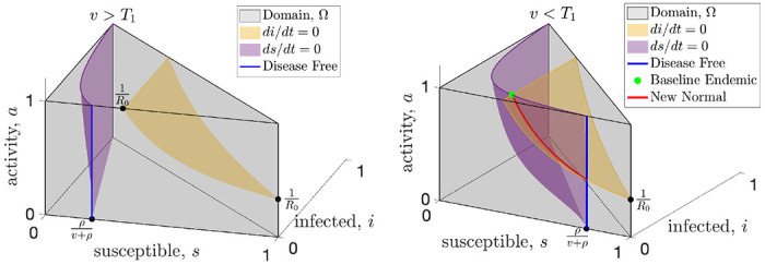
When vaccine rates are sufficiently high (left panel), the only equilibrium is disease-free (blue) and resilience will drive the activity to baseline which is the top of the blue line. When vaccination rates drop below the critical threshold (right panel), the baseline endemic equilibrium (green dot) is created, along with at least one new normal endemic equilibrium along the red curve.
First, we examine the equilibria which will determine the possible long-term characteristics of the disease. An equilibria means that none of the variables are changing, so to find the equilibria we set (8) equal to zero. We can visualize this in Fig. 1 which shows the surfaces where the infected population (yellow) and the susceptible population (purple) are instantaneously not changing. And equilibrium can only happen at the intersection of these two surfaces, or where the purple surface intersects the i = 0 plane (disease-free). When the vaccination rate is sufficiently high, as shown in the left panel of Fig. 1, the surfaces do not intersect and the only equilibrium is disease-free. In the right panel of Fig. 1 we see that when the vaccination rate is lower the surfaces intersect and new equilibria are possible at the green dot (endemic with baseline behavior, a = 1) or along the red curve (new normal endemic, a < 1). In Fig 2 we show horizontal slices of the region in Fig. 1 which represent the dynamics at a fixed activity level. The cross sections of the surfaces in Fig. 1 appear as curves in Fig. 2. When the vaccination rate is greater than T1 the curves do not intersect and the only equilibrium is disease free as shown in the left panel of Fig. 2. When the vaccination rate is less than T1 the curves intersect at a baseline activity level (middle panel of Fig. 2) and at least one new normal equilibrium (right panel).
FIG. 2:
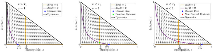
Here we show three horizontal slices (fixed activity slices) from the domain, , shown in Fig. 1. The left and middle slices show the top of the domain (a = 1) with high and moderate vaccination rates respectively. The right slice is from the middle of the domain when the vaccination rate is very low and only the new normal endemic is stable. Note that the flow arrows, curves, and intersections shown in these cross sections depend on the disease parameters but are independent of the behavioral dynamics (except for the activity level, a, of the new normal endemic shown in the right panel).
To see this mathematically, setting immediately implies that either i = 0 or . The former case is the disease-free equilibrium, and, in the latter case, one can show that the fraction of the infected population will be,
| (9) |
This cannot be negative, and since the first term in the numerator is negative or zero, so we immediately see that when the vaccination rate is greater than there cannot be any equilibria of the form (9). At this point we have only made Assumption A1, and we already have a universal vaccination threshold which we call,
| (10) |
When the vaccination rate is above T1, the only possible equilibrium is the disease-free equilibrium, and this holds for any reactivity function F.
Next we turn to the stability of the disease-free equilibrium, and for that we will need to assume resilience. Resilience assumes that when incidence is zero (as in the disease-free situation) and activity is less than baseline, then activity will increase. While this seems intuitive it does not imply stability by itself. The reason is that we are only making an assumption about what happens when incidence is zero. Stability requires that even if we perturb the disease-free equilibrium by introducing a small number of infections, the system must return to the disease-free equilibrium. In Theorem 3 in the supplement, we prove that the disease free equilibrium is in fact stable, as long as the vaccination rate is above T1. So for any resilient behavioral response, a vaccination rate above T1 guarantees not only that the disease-free equilibrium is the only equilibrium, but also that it is stable.
When the vaccination rate drops below the universal threshold T1, the disease-free equilibrium becomes unstable, and endemic equilibria become possible with infection rates given by (9). So now the question becomes, is it possible to have an endemic equilibrium with baseline activity? Setting a = 1 (baseline activity) in (9), we see that this is indeed possible since v is now less than T1 making the numerator of (9) positive. This means that there is a constant low level of infection given by (9), and so there must also be a constant low level of incidence, c > 0. For a baseline endemic equilibrium to exist, we only require that normal activity be stationary for this incidence level, meaning that F(1, c) = 0. Not every reactivity function, F, will have a baseline endemic equilibrium, and we give several examples in Section IV of reactivity functions that show the range of possibilities.
While not as desirable as a disease-free equilibrium, an endemic equilibrium with baseline activity (a = 1) may still be preferred to permanently modifying behavior, so it is important to determine the stability of this endemic equilibrium. The results above have only required us to assume that the behavior is reactive and resilient; however, now we will now require our final assumption of boundedness. Recall that a bounded behavioral response limits the average activity, a, to be at most the baseline level of activity, which is defined as a = 1, by imposing (6). In Theorem 4 in the supplement, we show that for any bounded behavioral response, there will be a second vaccination threshold, T2, which determines the stability of the baseline endemic equilibrium. The T2 threshold is derived in the supplement and is given by,
| (11) |
where is a constant that depends on the properties of the reactivity function, F, near the baseline endemic equilibrium. The constant will often be positive, and in these cases the T2 vaccination threshold will be lower than the T1 threshold. In these cases, when the vaccination rate is higher than T2 but less than T1, the baseline endemic endemic will be stable. On the other hand, for some reactivity functions, the constant can be negative or zero, and for these reactivity functions the baseline endemic equilibrium will not be stable for any vaccination rate. Once the reactivity function, F, is specified, T2 can be computed explicitly and we show how to compute T2 along with several examples in the Supplementary Material. This shows that even when the classical threshold for effective vaccination cannot be achieved, there can still be a substantial benefit in a lower vaccination rate. As long as the vaccination rate exceeds the new T2 threshold, the baseline activity level will be stable (see examples in Fig. 3).
FIG. 3:
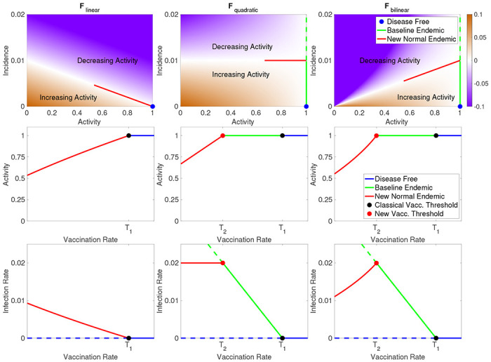
In the top row we illustrate each of the three example behavioral response functions introduced in Section IV. In the respective column for each response function, we show the equilibrium activity, a (middle row), and infection rate, i (bottom row), as functions of vaccination rate, v. When v > T1 we have the disease-free equilibrium (blue), and for v between T2 and T1 we have the baseline endemic (green), and when v < T2 the new normal endemic equilibrium. Solid lines reflect stable equilibria, and dotted lines unstable.
Finally, we consider what happens when the vaccination rate is less than both the T1 and T2 thresholds. In particular, this will typically be the case in the early stages of a novel disease when a vaccination has not been developed and v = 0. In this situation, both the disease-free equilibrium and the baseline endemic become unstable, so there is no stable equilibrium with baseline activity. However, this does not immediately imply the existence of a new normal equilibrium, for example the dynamics might fall into a periodic cycle or even behave chaotically. While these more exotic dynamics are indeed possible, in Theorem 6 in the supplement we prove that there is at least one new normal equilibrium.
IV. EXAMPLES
We emphasize that our results apply to any response function F that satisfies A1 - A3. However, to illustrate of our results we introduce three simple resilient and bounded models for F.
| (12) |
| (13) |
| (14) |
These functions all satisfy resilience and boundedness for any w1, w2 > 0 and we illustrate them in the top row of Fig. 3 for w1 = 0.1 and w2 = 10. The first two functions above are important because they are the leading order approximation of any response function. Note that the function Fquadratic is quadratic in a since c = aBsi and similarly Fbilinear is bilinear in a and i. In the Supplement we show how to analyze each of these models using our theoretical results, including finding the vaccination thresholds, T1 and T2, as well as determining how the new normal equilibria depend on the vaccination rate. In particular we show that the simplest model, Flinear, does not have an baseline endemic because T2 = T1. On the other hand, both Fquadratic and Fbilinear have T2 < T1, so for vaccination rates between these thresholds the baseline endemic is stable.
The primary difference between the three example behavioral response functions is how quickly the equilibrium level of activity falls off as vaccination rate decreases, as shown in the top row Fig. 3. For Flinear the activity vs. vaccination curve is convex, and this moderate response results in a new normal infection rate that increases rapidly as vaccination rate decreases as shown in the bottom row of Fig. 3. In the Fquadratic model, equilibrium activity decreases linearly with vaccination rate and this model has the interesting feature that the decrease in activity exactly balances the decrease in vaccination rate leading to a constant level infection rate in the new normal endemic even as vaccination rates fall. Finally, Fbilinear has the most robust behavioral response, with a concave drop in activity as vaccination rate decreases. This response results in infection rate actually falling as vaccination rates decline. While this may seem counter-intuitive, it is caused by the lack of vaccination causing the system to find a new equilibrium with much lower activity levels which in turn result in lower infection rates. This is particularly interesting because it shows how when initially introducing a vaccination to a population the infection rate may initially increase until the critical vaccination rate threshold T2 is reached and the baseline endemic is stabilized. This will especially be the case for a new vaccination that is being gradually rolled out, since a slow change in the vaccination rate will help keep the system near equilibrium as the new normal shifts.
While we suggest that these are reasonable first approximations and have many interesting characteristics, we make no attempt to justify these as models for behavior and provide them purely as examples, since our results apply to all possible resilient and bounded models.
Before concluding we note a fascinating feature of Fbilinear. If we consider s as approximately constant and set d = 1 − a then (8) becomes,
| (15) |
which is exactly the Lotka-Volterra predator-prey model. Perhaps counter-intuitively, in this analogy the infections play the role of prey and ‘distancing’, d, plays the role of the predator. Regardless of the analogy, the interesting feature of this model is that it produces oscillations with frequency . This approximation is valid when these activity driven oscillations are fast enough that s is approximately constant over the course of an oscillation. Each oscillation reduces s slightly, and over time the frequency decreases. Eventually, when , we have which changes the stability of the equilibrium inside the periodic orbit of (15) from a center to a source. Thus, represents a phase transition threshold for this model.
V. DISCUSSION
In this article, we have proposed a simple way to include social activity effects in the influential SIR model, allowing a wide range of functional forms of response. Under these assumptions, we have shown that for a broad range of behavioral feedbacks between the incidence of infection and activity that contributes to transmission (e.g. contact rates or hygiene) there exist two novel equilibria in addition to the classic vaccine-based herd immunity threshold. These results have important implications for the role of vaccination and behavioral interventions in pathogen elimination and eradication. First, while coordinated behavioral interventions may be sufficient to drive incidence to 0, e.g. as was seen for SARS-CoV-1 and Ebola outbreaks prior to 2017, such interventions alone cannot stabilize the disease-free equilibrium if behavior adheres to the resilience property. In the absence of vaccination there are no stable equilibria that have a return to normal activity. SARS-CoV-1 is the rare example of a pathogen that emerged and was eradicated (driven to 0 prevalence globally) in the absence of a vaccine; however, reintroduction from an animal reservoir remains possible [24] and the relaxation of the behavioral interventions instituted to achieve elimination [7] make the current disease-free state unstable [23].
In our model with behavioral feedbacks, vaccination at or above the classic herd immunity threshold (T1) is sufficient to stabilize the disease-free equilibrium for all behavioral responses, making elimination (locally) or eradication (globally) robust to re-introduction or re-emergence. Vaccination below this threshold is insufficient to stabilize a disease-free state even if behavior is reduced at equilibrium; vaccination below a newly identified threshold (T2) leads to a stable equilibrium where the prevalence of infection is non-zero and behavior is stable at a new level of activity that is below the disease-free level: the “new-normal”. We identify a new regime where vaccination is above T2 and below T1 where the incidence of infection is stable and activity will be stable at normal (disease-free) levels. The only stable equilibrium with vaccination below T2 results in stable reduction of activity (a < 1). Such a reduction could take the form of persistent reduction in activity levels or in additional avoidance behaviors such as masking or hygiene.
The newly identified regime with vaccination between T2 and T1 has substantial policy implications for emerging infections and eradication efforts. In the absence of pre-existing vaccines, non-pharmaceutical interventions (NPIs) are likely to be an important part of pandemic response for emerging infections; as was the case for SARS-CoV-2. Such NPIs can be onerous and lead to significant off-target effects. The SARS-COV-2 pandemic led to dramatic economic [11] and educational [17, 18] consequences. Planning for a safe return to pre-emergence activity can minimize these off-target effects. We show that vaccination at a level T2 that is lower than the classic herd immunity threshold T1 can permit a return to pre-emergence activity while maintaining a stable, non-zero incidence. While total elimination or eradication may still be a goal, these results suggest that a return to pre-emergence activity can proceed at a level of vaccination below T1. Further, while attaining T1 may be challenging in may settings, particularly in the face of vaccine hesitancy or uncertainty about the rate of vaccine waning, the existence of T2 suggests a midpoint goal for vaccination rate that can be used to motivate vaccination efforts.
The existence of the vaccination regime between T2 and T1 may further be useful in development of policies for eradication of endemic infections. The only benefits to vaccination in the standard SIR modeling framework without behavioral feedbacks are reductions in morbidity and mortality. These benefits accrue in a near linear fashion when vaccination rates are low and accelerate dramatically in the vicinity of T1. This new model implies additional societal change, in the form of the increased activity, that may be stabilized at or above T2. Whether this represents a societal benefit or not will be highly system specific. For example, vaccination rates above T2 may allow for relaxation of prescreening requirements and the costs inherent in such programs. Alternatively, one could imagine an increase in risky behaviors, e.g. decreased mask usage as SARS-CoV-2 vaccination increases, that could then facilitate an increase in other respiratory infections. Any specific predictions of such phenomena is speculative without a mechanistic understanding of the explicit nature of the feedbacks. For example Funk et al. [16] considered that information, and thus behavioral response, may only be available locally rather than globally and Weitz et al. [29] considered that behavioral response may react to the incidence of mortality rather than infection. The general extension of the classic compartmental modeling framework for infectious diseases that we have proposed opens the door for a formal theory of such host-pathogen-behavioral dynamics to guide more specific mechanistic investigations.
The description of these new equilibria represents a critical advance for infectious disease and vaccination policy development. A stable equilibrium provides a policy target where the system is self-managing and self-maintaining. The existence of such a stable target allows optimal policy strategies to be formulated to reach that point. Policy formulation without such an explicit goal requires iterative trial-and-error which may incur economic or societal costs that can undermine support for the process. Such adaptive control strategies built upon iterative learning have a long history [19, 27, 30] and are useful tools complemented by our results showing that there are multiple advantageous stable equilibria (either disease-free or endemic) allowing a return to normal behavior. In the face of uncertainty about the feasibility of elimination, the endemic state with return to normal behavior provides a valuable new policy target that can be used to motivate action and guide the development of research on behavioral feedback to support policy planning.
Supplementary Material
Acknowledgments:
Supported by US NIH Director’s Transformative Award 1R01AI145057.
References
- [1].Anderson Roy M and May Robert M. Infectious diseases of humans: dynamics and control. Oxford university press, 1992. [Google Scholar]
- [2].Arthur Ronan F, Jones James H, Bonds Matthew H, Ram Yoav, and Feldman Marcus W. Adaptive social contact rates induce complex dynamics during epidemics. PLoS computational biology, 17(2):e1008639, 2021. [DOI] [PMC free article] [PubMed] [Google Scholar]
- [3].Ash Thomas, Bento Antonio M, Kaffine Daniel, Rao Akhil, and Bento Ana I. Disease-economy trade-offs under alternative epidemic control strategies. Nature Communications, 13(1):1–14, 2022. [DOI] [PMC free article] [PubMed] [Google Scholar]
- [4].Bauch Chris, d’Onofrio Alberto, and Manfredi Piero. Behavioral epidemiology of infectious diseases: an overview. Modeling the interplay between human behavior and the spread of infectious diseases, pages 1–19, 2013. [Google Scholar]
- [5].Bauch Chris T and Earn David JD. Vaccination and the theory of games. Proceedings of the National Academy of Sciences, 101(36):13391–13394, 2004. [DOI] [PMC free article] [PubMed] [Google Scholar]
- [6].Begon Michael, Bennett Malcolm, Bowers Roger G, French Nigel P, Hazel SM, and Turner Joseph. A clarification of transmission terms in host-microparasite models: numbers, densities and areas. Epidemiology & Infection, 129(1):147–153, 2002. [DOI] [PMC free article] [PubMed] [Google Scholar]
- [7].Bell David M et al. Public health interventions and sars spread, 2003. Emerging infectious diseases, 10(11):1900, 2004. [DOI] [PMC free article] [PubMed] [Google Scholar]
- [8].Bonaccorsi Giovanni, Pierri Francesco, Cinelli Matteo, Flori Andrea, Galeazzi Alessandro, Porcelli Francesco, Schmidt Ana Lucia, Valensise Carlo Michele, Scala Antonio, Quattrociocchi Walter, et al. Economic and social consequences of human mobility restrictions under covid-19. Proceedings of the National Academy of Sciences, 117(27):15530–15535, 2020. [DOI] [PMC free article] [PubMed] [Google Scholar]
- [9].Buckee Caroline O, Balsari Satchit, Chan Jennifer, Crosas Mercè, Dominici Francesca, Gasser Urs, Grad Yonatan H, Grenfell Bryan, Halloran M Elizabeth, Kraemer Moritz UG, et al. Aggregated mobility data could help fight covid-19. Science, 368(6487):145–146, 2020. [DOI] [PubMed] [Google Scholar]
- [10].Buonomo Bruno, d’Onofrio Alberto, and Lacitignola Deborah. Global stability of an sir epidemic model with information dependent vaccination. Mathematical biosciences, 216(1):9–16, 2008. [DOI] [PubMed] [Google Scholar]
- [11].Chen Jiangzhuo, Vullikanti Anil, Santos Joost, Venkatramanan Srinivasan, Hoops Stefan, Mortveit Henning, Lewis Bryan, You Wen, Eubank Stephen, Marathe Madhav, et al. Epidemiological and economic impact of covid-19 in the us. Scientific reports, 11(1):1–12, 2021. [DOI] [PMC free article] [PubMed] [Google Scholar]
- [12].Epstein Joshua M, Parker Jon, Cummings Derek, and Hammond Ross A. Coupled contagion dynamics of fear and disease: mathematical and computational explorations. PloS one, 3(12):e3955, 2008. [DOI] [PMC free article] [PubMed] [Google Scholar]
- [13].Fenichel Eli P, Castillo-Chavez Carlos, Ceddia M Graziano, Chowell Gerardo, Gonzalez Parra Paula A, Hickling Graham J, Holloway Garth, Horan Richard, Morin Benjamin, Perrings Charles, et al. Adaptive human behavior in epidemiological models. Proceedings of the National Academy of Sciences, 108(15):6306–6311, 2011. [DOI] [PMC free article] [PubMed] [Google Scholar]
- [14].Ferrari Matthew J, Grais Rebecca F, Bharti Nita, Conlan Andrew JK, Bjørnstad Ottar N, Wolfson Lara J, Guerin Philippe J, Djibo Ali, and Grenfell Bryan T. The dynamics of measles in sub-saharan africa. Nature, 451(7179):679–684, 2008. [DOI] [PubMed] [Google Scholar]
- [15].Fine Paul EM and Clarkson Jacqueline A. Measles in england and wales—i: an analysis of factors underlying seasonal patterns. International journal of epidemiology, 11(1):5–14, 1982. [DOI] [PubMed] [Google Scholar]
- [16].Funk Sebastian, Gilad Erez, Watkins Chris, and Jansen Vincent AA. The spread of awareness and its impact on epidemic outbreaks. Proceedings of the National Academy of Sciences, 106(16):6872–6877, 2009. [DOI] [PMC free article] [PubMed] [Google Scholar]
- [17].Hammerstein Svenja, König Christoph, Dreisörner Thomas, and Frey Andreas. Effects of covid-19-related school closures on student achievement-a systematic review. Frontiers in psychology, 12:746289, 2021. [DOI] [PMC free article] [PubMed] [Google Scholar]
- [18].Hoofman Jacob and Secord Elizabeth. The effect of covid-19 on education. Pediatric Clinics, 68(5):1071–1079, 2021. [DOI] [PMC free article] [PubMed] [Google Scholar]
- [19].Keith David A, Martin Tara G, McDonald-Madden Eve, and Walters Carl. Uncertainty and adaptive management for biodiversity conservation, 2011. [Google Scholar]
- [20].Kermack William Ogilvy and McKendrick Anderson G. A contribution to the mathematical theory of epidemics. Proceedings of the royal society of london. Series A, Containing papers of a mathematical and physical character, 115(772):700–721, 1927. [Google Scholar]
- [21].Lau Max SY, Grenfell Bryan, Thomas Michael, Bryan Michael, Nelson Kristin, and Lopman Ben. Characterizing superspreading events and age-specific infectiousness of sars-cov-2 transmission in georgia, usa. Proceedings of the National Academy of Sciences, 117(36):22430–22435, 2020. [DOI] [PMC free article] [PubMed] [Google Scholar]
- [22].Lowen Anice C and Steel John. Roles of humidity and temperature in shaping influenza seasonality. Journal of virology, 88(14):7692–7695, 2014. [DOI] [PMC free article] [PubMed] [Google Scholar]
- [23].Monaghan Karen. SARS: Down but still a threat, volume 3. National Intelligence Council, 2003. [Google Scholar]
- [24].Morens David M and Fauci Anthony S. Emerging pandemic diseases: how we got to covid-19. Cell, 182(5):1077–1092, 2020. [DOI] [PMC free article] [PubMed] [Google Scholar]
- [25].Reluga Timothy C. Game theory of social distancing in response to an epidemic. PLoS computational biology, 6(5):e1000793, 2010. [DOI] [PMC free article] [PubMed] [Google Scholar]
- [26].Rizzo Alessandro, Frasca Mattia, and Porfiri Maurizio. Effect of individual behavior on epidemic spreading in activity-driven networks. Physical Review E, 90(4):042801, 2014. [DOI] [PubMed] [Google Scholar]
- [27].Shea Katriona, Tildesley Michael J, Runge Michael C, Fonnesbeck Christopher J, and Ferrari Matthew J. Adaptive management and the value of information: learning via intervention in epidemiology. PLoS biology, 12(10):e1001970, 2014. [DOI] [PMC free article] [PubMed] [Google Scholar]
- [28].Tkachenko Alexei V, Maslov Sergei, Wang Tong, Elbana Ahmed, Wong George N, and Goldenfeld Nigel. Stochastic social behavior coupled to covid-19 dynamics leads to waves, plateaus, and an endemic state. Elife, 10:e68341, 2021. [DOI] [PMC free article] [PubMed] [Google Scholar]
- [29].Weitz Joshua S, Park Sang Woo, Eksin Ceyhun, and Dushoff Jonathan. Awareness-driven behavior changes can shift the shape of epidemics away from peaks and toward plateaus, shoulders, and oscillations. Proceedings of the National Academy of Sciences, 117(51):32764–32771, 2020. [DOI] [PMC free article] [PubMed] [Google Scholar]
- [30].Williams Byron K. Adaptive management of natural resources—framework and issues. Journal of environmental management, 92(5):1346–1353, 2011. [DOI] [PubMed] [Google Scholar]
- [31].Wormser Gary P and Pourbohloul Babak. Modeling infectious diseases in humans and animals by matthew james keeling and pejman rohani princeton, nj: Princeton university press, 2008. 408 pp., illustrated., 2008. [Google Scholar]
Associated Data
This section collects any data citations, data availability statements, or supplementary materials included in this article.