

Abstract
Quantitative Susceptibility Mapping (QSM) is an established Magnetic Resonance Imaging (MRI) technique with high potential in brain iron studies associated to several neurodegenerative diseases. Unlike other MRI techniques, QSM relies on phase images to estimate tissue’s relative susceptibility, therefore requiring a reliable phase data. Phase images from a multi-channel acquisition should be reconstructed in a proper way. On this work it was compared the performance of combination of phase matching algorithms (MCPC3D-S and VRC) and phase combination methods based on a complex weighted sum of phases, considering the magnitude at different powers (k = 0 to 4) as the weighting factor. These reconstruction methods were applied in two datasets: a simulated brain dataset for a 4-coil array and data of 22 postmortem subjects acquired at a 7T scanner using a 32 channels coil. For the simulated dataset, differences between the ground truth and the Root Mean Squared Error (RMSE) were evaluated. For both simulated and postmortem data, the mean (MS) and standard deviation (SD) of susceptibility values of five deep gray matter regions were calculated. For the postmortem subjects, MS and SD were statistically compared across all subjects. A qualitative analysis indicated no differences between methods, except for the Adaptive approach on postmortem data, which showed intense artifacts. In the 20% noise level case, the simulated data showed increased noise in central regions. Quantitative analysis showed that both MS and SD were not statistically different when comparing k = 1 and k = 2 on postmortem brain images, however visual inspection showed some boundaries artifacts on k = 2. Furthermore, the RMSE decreased (on regions near the coils) and increased (on central regions and on overall QSM) with increasing k. In conclusion, for reconstruction of phase images from multiple coils with no reference available, alternative methods are needed. In this study it was found that overall, the phase combination with k = 1 is preferred over other powers of k.
Keywords: Magnetic resonance imaging, Quantitative susceptibility mapping, MRI phase reconstruction, Postmortem
Introduction
In recent years, Quantitative Susceptibility Mapping (QSM) has been highly applied on neurodegenerative diseases’ studies due to its capability of quantitatively infer tissue’s relative susceptibility [5,17,23]. It has been shown that susceptibility values in the basal ganglia are highly correlated to total iron concentration [2,7,24], while for white matter, myelin seems to be the predominant source, giving rise to anisotropic susceptibility [8–10,24].
The tissue’s bulk magnetic susceptibility distribution can be estimated by using the phase images from a gradient echo experiment. At a given echo time TE, the local accumulated phase is proportional to the local magnetic field :
| (1) |
Therefore, an essential condition for an adequate QSM processing is an optimized Signal-to-Noise Ratio (SNR) of the raw phase images. More than three decades ago, the use of phased array radiofrequency coils improved the SNR when compared to volume coils, allowing faster acquisitions [20]. The image acquisition speed involving array coils has also been accelerated using several signal reconstructions approaches in the last two decades, nevertheless focused on magnitude images.
For a multi-channel acquisition, signal from multiple coils is acquired and then combined into a single image. Then, magnitude and phase information are obtained from the combined signal. Reconstruction methods used by the scanner are optimized for magnitude images but may be sub-optimal for phase images [3,21].
Unlike magnitude, phase images from individual coils also contains offset terms which adds up to the measured phase. This can result on signal cancellation and propagate artifacts on reconstructed phase images if not corrected [18]. Additionally, phase from each coil should be combined by means of a sum of the complex signal or a sum of phases, which should also account for the SNR distribution of each coil, usually applied as a weighting factor during the combination step. Therefore, phase reconstruction should follow mainly two steps: the phase offset correction (referred here as Matching Phase step); and Phase Combination step.
Different phase combination methods from multiple coils have been proposed and evaluated [4,6,13,19]. These studies used a weighted sum of the complex signal, or a weighted sum of the phases, with weights based on the SNR profile of each coil. The weighting factor used on these studies were based on magnitude images, and two powers of magnitude images were used for the sum of phases: k = 1 and k = 2, but no comparison between each power were made. Moreover, high order weighting (k > 2) and the effect of these methods on QSM maps have not been evaluated yet.
Methods that aim to estimate the phase offset were also evaluated in the literature. [18] explored the quality of phase maps which were offset corrected with different approaches. However, no further QSM analysis was made in order to better evaluate the impact each method had on susceptibility maps, specifically when looking on specific brain regions. [1] compared the impact different offset correction methods had on phase maps, focusing on QSM application. Their results showed differences between methods, which implies that the choice of phase reconstruction method can alter the resulting QSM, but no region-specific analysis was made.
Abdulla and collaborators also found that a multi-echo approach for offset estimation is dependent on the choice of TEs for its estimation [1]. This implies that the linear dependence (Eq. 1) for phase evolution does not hold, and therefore can affect the results. On the other hand, a single-echo approach does not rely on this assumption. Indeed, the authors found that single-echo approach resulted on lower standard deviation of susceptibility values on evaluated ROIs, which indicates that QSM maps reconstructed from single-echo offset corrected phase maps presented a higher uniformity.
Region-specific analysis is essential when evaluating the resulting QSM maps since most applications of QSM relies on specific brain regions. Additionally, on postmortem condition there’s significant changes that can alter the susceptibility distribution, such as the presence of fully deoxygenated blood and myelin degradation. These effects are accentuated on phase images and must be taken into consideration. On the other hand, movement artifacts are not present in postmortem images reducing dynamic partial volume effect in the tissue boundaries. Evaluation of different processing steps of QSM (background field removal and dipole inversion) on postmortem images were already made [22], however there has not been a proper evaluation of phase reconstruction methods for postmortem data.
Therefore, our main goal is to compare the effect of different phase reconstruction methods in the susceptibility maps for two datasets: simulated brain data and postmortem data acquired in a 7T scanner. Based on the maps, we perform qualitative and quantitative comparison considering global metrics and specific brain regions.
Methods
MCPC3D-S offset correction approach
The phase at the position in the raw phase image from a single coil acquired using a TE echo time can be modelled considering the contribution of three terms: phase evolution of the sample’s magnetization ( from Eq. 1), an offset term which is intrinsic to the coil’s configuration , and noise .
| (2) |
The first term is common to all coils and corresponds to the true phase of the sample. The second term is specific for each coil and should be corrected prior to signal combination since these terms can generate phase artifacts which compromises the reconstructed phase images.
The term can be estimated by considering the temporal evolution of phase images as given by Eq. 1. With the phase from two different echo times (TE1 and TE2), the offset term can be expressed as (MCPC3D method):
| (3) |
However, since phase images are constrained to 2π interval, phase wraps can add additional terms into Eq. 3, and degrade the quality of phase images. Therefore, phase images must be unwrapped in order to apply the MCPC3D method.
Eq. 3 can be rewritten in the following way:
| (4) |
This way, only the phase difference between echo 1 and echo 2 should be unwrapped . This method (MCPC3D-S) results in an improved computer performance and reduces artifacts when compared to the MCPC3D method [4].
Furthermore, if the echo times are chosen so that TE2 = (m+1)TE1 (ASPIRE method), the unwrapping step can be skipped, improving even more the computer performance and quality of phase images [4].
Finally, phase from each coil can be corrected by the offset factor by subtracting from the measured phase :
| (5) |
VRC approach
Multi-echo estimations of relies on the assumption that evolves linearly with time. This assumption seems to breakdown since choosing different TE1 and TE2 can lead to different estimations [1]. Additionally, if wrapped phases are not properly unwrapped, then the estimation is not accurate.
Phase matching can also be performed using single echo phase images by referencing each coil into a reference image. In this way, the offset of each coil is substituted by the offset of the reference image. Specially for ultra-high fields, a reference image is not available and therefore a virtual image can be used as a reference [15,16]. The virtual image should contain high SNR over the entire volume so that noise amplification can be minimized when referencing the coils. A proper choice of can be the complex-weighted sum of phase of each coil :
| (6) |
Where accounts for the SNR distribution of each coil and ∅0 is chosen so that the phase of all channels cancels all at a reference region (usually the center of the image). This way one can ensure that the has enough SNR over the entire volume. The now can be modelled as:
| (7) |
Where will contain the true phase distribution , an offset term and a noise distribution :
| (8) |
Now can be subtracted from , resulting on a phase difference :
| (9) |
This phase difference will only contain the differences on the offset of each coil, and the differences in the noise. By applying a low-pass filter, the noise term can be suppressed, resulting on a difference of offset terms. By adding back to the phase of each coil, the , is removed and replaced by . This way, all coils will have the same offset .
It should be noted that this approach, called Virtual Reference Coil (VRC) does not eliminate the offset term. Instead, it replaces the offset of each channel by a common offset. This can overcome the effects of artifact propagation when combining phase, however it should be noted that this offset term will still be carried out on the resulting constructed phase. For QSM processing, this additional term can then be suppressed during the phase adjustment step.
Phase combination using weighted-sum
After the phase matching step, signals from all coils are combined in order to generate a single signal , resulting on a reconstructed phase image. The combination step is also important since can interfere with the resulting images.
Each coil has its own spatial sensitivity, and therefore, its own SNR spatial distribution over the volume. If this distribution is not considered, contributions from coils with low SNR can propagate to the resulting combined images, decreasing overall quality.
Reconstructed signal can be achieved by means of a weighted sum of the complex signal, which was previously phase matched, of each coil , with a weighting factor , which weights over the coil’s sensitivity:
| (10) |
Where the index k′ is responsible to increase the weighting over the local SNR. Ignoring noise correlation between coils, and assuming a Gaussian distribution for the noise of each coil, then magnitude images can be used as weighting factor:
| (11) |
By using the magnitude as a weighting factor, signal from regions of a coil with low SNR are suppressed, while regions with high SNR are amplified.
Furthermore, can be understood as a combination of both magnitude and phase information:
| (12) |
This way, can be rewritten in terms of a weighted sum of the phase :
| (13) |
Where contains and incorporates the term from , resulting in:
| (14) |
Where .
Previous papers have used k = 1 [6,19] and k = 2 [4] for the weighting factors, however no further comparison between linear or quadratic weighting was made. Furthermore, evaluations using higher k values have not been reported yet.
By increasing k, local phase from coils with higher SNR are further amplified in contrast to those with lower SNR, i.e. it can further suppress noise while helping give a more precise estimative of the phase distribution. In the limiting case (k→∞), the phase can be taken to be that of the coil with the highest signal among all coils, while this is optimal for regions near the coil (where there’s a maximum SNR for that coil), this is compensated by lowering SNR of regions that are relatively far from all coils, i.e., the center of the volume. In summary, increasing the value of k is a trade-off between SNR of regions near the coils, and regions appreciable far from all coils (center of the volume).
In this work we vary the exponent k from 0 to 4 (where 0 represents a simple phase sum) to explore how the weighting factor during the combination step can influence QSM maps. On the other hand, the use of only one term in the sum, considering the coil with highest magnitude signal, represents a condition with large k value (k→∞).
Simulated dataset
To generate the simulated dataset, a box was created, representing the whole image, in which the object of interest and the coils would be positioned. The size of the image was chosen so that it would be approximately 2 times the size of the object. Four identical circular coils (Radius=1 cm) were generated, with different positions and orientations relative to the object. These orientations were chosen so that their normal would be perpendicular to the z-axis (axial direction), and their position relative to the head were: frontal, occipital, left and right positions. Then, magnetic field distribution for each coil was calculated by means of a 3D convolution operation of the current density and the function , given by the Biot-Savart law (Eq. 15). The magnetic field distribution of each coil was used to determine their respective spatial sensitivity. It is worth mentioning that radiofrequency inhomogeneity was not incorporated in these simulations.
| (15) |
| (16) |
Finally, the resulting signal acquired by the C-th coil was generated using the following:
| (17) |
Where, and are the ground truth of magnitude and phase images. and are the absolute value of the x and y component of the magnetic field of the C-th coil, and is an artificial gaussian noise generated for this coil.
A digital head phantom was defined as the object of interest. This head phantom consisted of simulated phase and magnitude images [14], which were used as a ground truth. The phantom also contained the ground truth QSM. By applying the contributions from each coil (transverse components of the magnetic field) into the ground truth images (magnitude and phase) complex signal for each coil were simulated following Eq. 17. Additive and uncorrelated gaussian noise was incorporated to the model and different noise level (5%, 10% and 20%) were considered. Fig. 1 shows one axial slice of the simulated images of phantom data from each coil assuming medium noise level (10%).
Fig. 1.
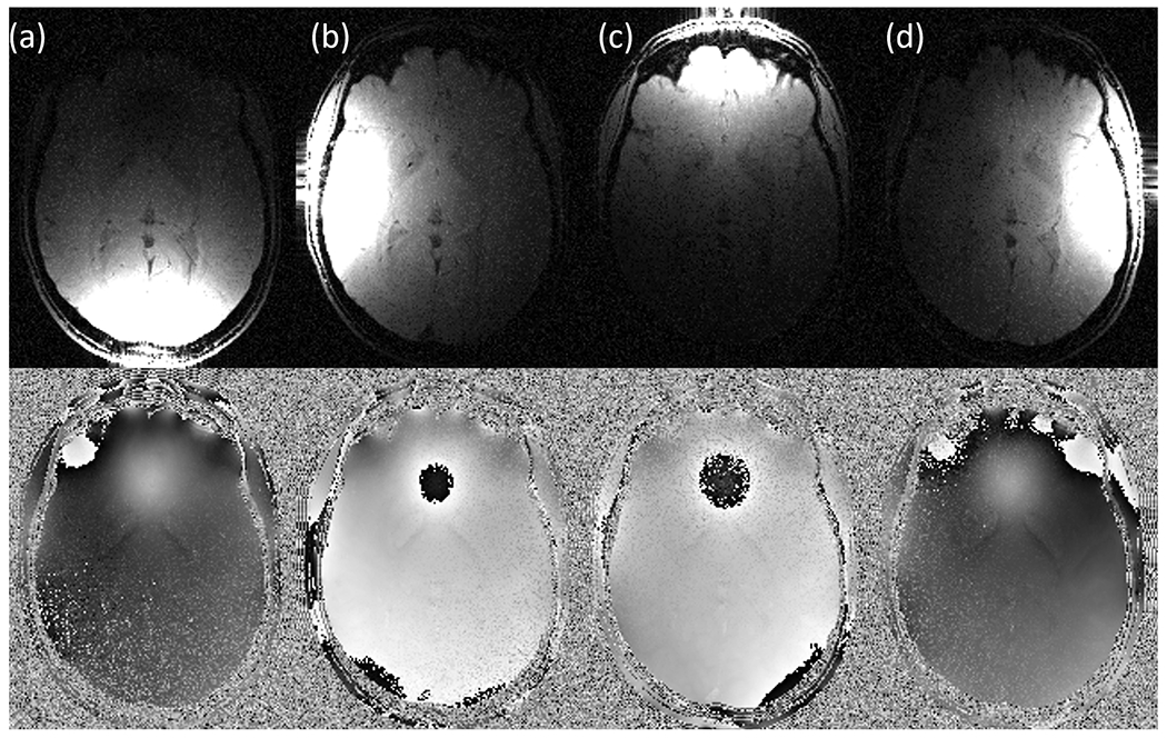
Simulated magnitude (top row) and phase (bottom row) images of the head phantom for each circular coil at different positions: a) Occipital, b) Right, c) Frontal, d) Left.
Acquired postmortem dataset
This study was approved by the research ethics’ committee of the Medicine School of the University of São Paulo, n° 14407. Postmortem MRI images from 22 subjects (ages between 51 and 91 years old; 13 males; without history of neurological diseases) were acquired from the Imaging Platform in the Autopsy Room (PISA) database. MRI was performed on a 7T MRI scanner (Magnetom, SIEMENS) with a 32 receiver channel head coil (Nova Medical, USA). An MP2RAGE sequence with 0.75 mm isotropic resolution and a multi-echo (n=5) gradient echo were acquired (1st TE/ΔTE = 5/4 ms; TR = 25ms; 0.5×0.5×1.0 mm3). For this study, magnitude and phase images from each channel were acquired and combined by offline reconstruction methods. Magnitude and phase images automatically reconstructed by the scanner with an Adaptative method (Walsh et al., 2000) were also used.
Image processing
The phase reconstruction was performed in two steps in the raw phase data of the channels:
Phase offset correction of each coil by means of MCPC3D-S [4] and VRC [15] methods. For the acquired postmortem data was also tested without this offset correction.
Coils’ signal reconstruction by means of a weighted phase sum with weighting factor considering the magnitude at different values of k (Eq. 10). For simulated data, k = 0 – 4 conditions and only considering the coil with higher signal (k→∞) were applied. For the acquired postmortem data, k = 1 and k = 2 conditions were used.
The resulting magnitude and phase images were processed in order to generate the QSM using the following pipeline (Fig. 2):
Phase adjusting using a non-linear fitting included in the MEDI toolbox [11]
Phase unwrapping using PRELUDE algorithm [11]
Background field removal using PDF algorithm [12]
Dipole inversion using MEDI-L1 algorithm [11]
Fig. 2.
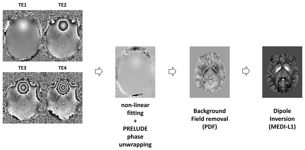
Main steps of QSM processing pipeline from the phase image acquired at different echo times to the susceptibility map.
For comparison, QSM were also obtained using the reconstructed postmortem images provided by the scanner.
Statistical analysis
For the postmortem dataset, five brain regions (Globus Pallidus, GP; Putamen, PUT; Caudate Nucleus, CN; Red Nucleus, RN; Substantia Nigra, SN) located at the basal ganglia were manually segmented on both sides (Fig. 3). Basal ganglia were chosen due to its high contrast in QSM images, and its relevance in neurodegenerative diseases associated to iron accumulation.
Fig. 3.
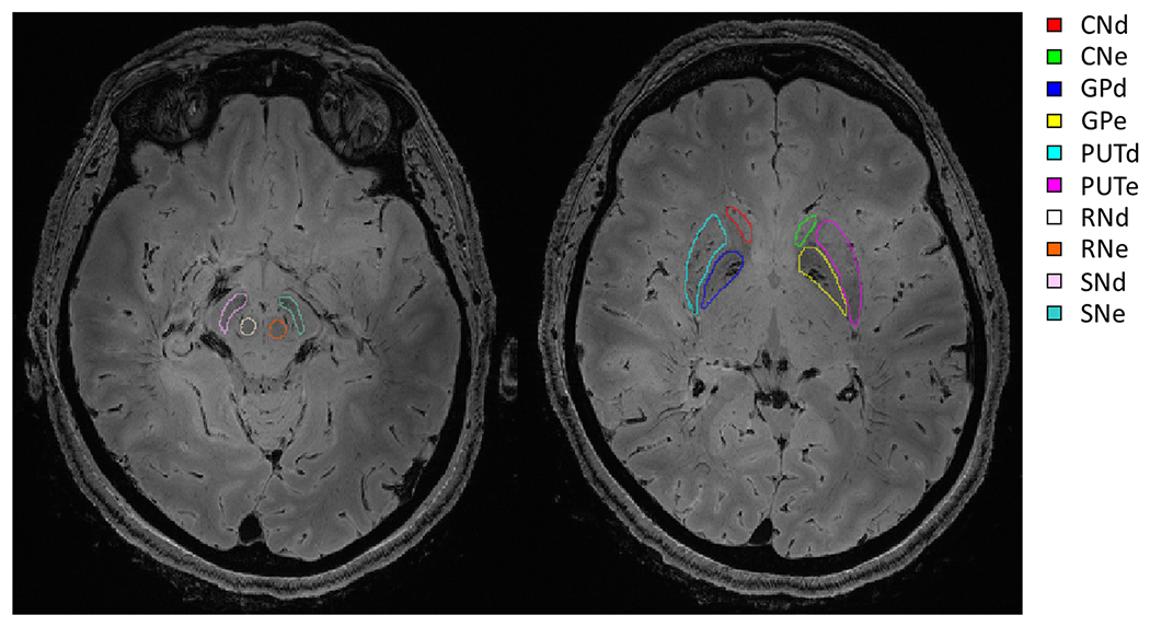
Examples of manually segmented basal ganglia ROIs in two axial slices on T2*-weighted magnitude image (scanner reconstruction) of one postmortem brain.
Mean susceptibility (MS) and standard deviation (SD) values were calculated in each segmented region in the susceptibility map for all subjects considering different reconstruction methods.
In a second-level analysis, MS and SD were calculated across all subjects, and then compared using a paired t-Student test and an ANOVA test. A correlation test and a Bland-Altman plot were also performed to evaluate the correlation and agreement between methods. For all statistical tests, significance level was defined at p<0,05.
For the reconstructed maps from simulated dataset, differences relative to the ground truth QMS were also calculated. From this difference, a root-mean square error (RMSE) was estimated for each phase reconstruction method used.
Additionally, the provided mask for Deep Gray Matter regions enabled the delineation of the same ROIs as in the postmortem case. Since the simulation consists of only one brain, the same analysis applied to postmortem dataset was not possible. However, the existence of a ground truth QSM in this case enables evaluation of the deviation relative to the ground truth on the estimative of QSM for each method.
Results
Simulated dataset
Results from the simulated dataset indicates only slight differences between methods with k = 1 – 4 (Fig. 4, Sup2). By ignoring the weighting factor (k = 0), resulting QSM maps shows lower SNR and higher difference to the ground truth at 5% and 10% noise levels compared to other k values. Considering only the voxels from the coil with the highest SNR (k→∞), when the noise level increases, the SNR from central region of the volume tends to decrease, however in regions near the coils seems to increase, while lowering the relative difference to the ground truth (Fig. 4, Sup2).
Fig. 4.
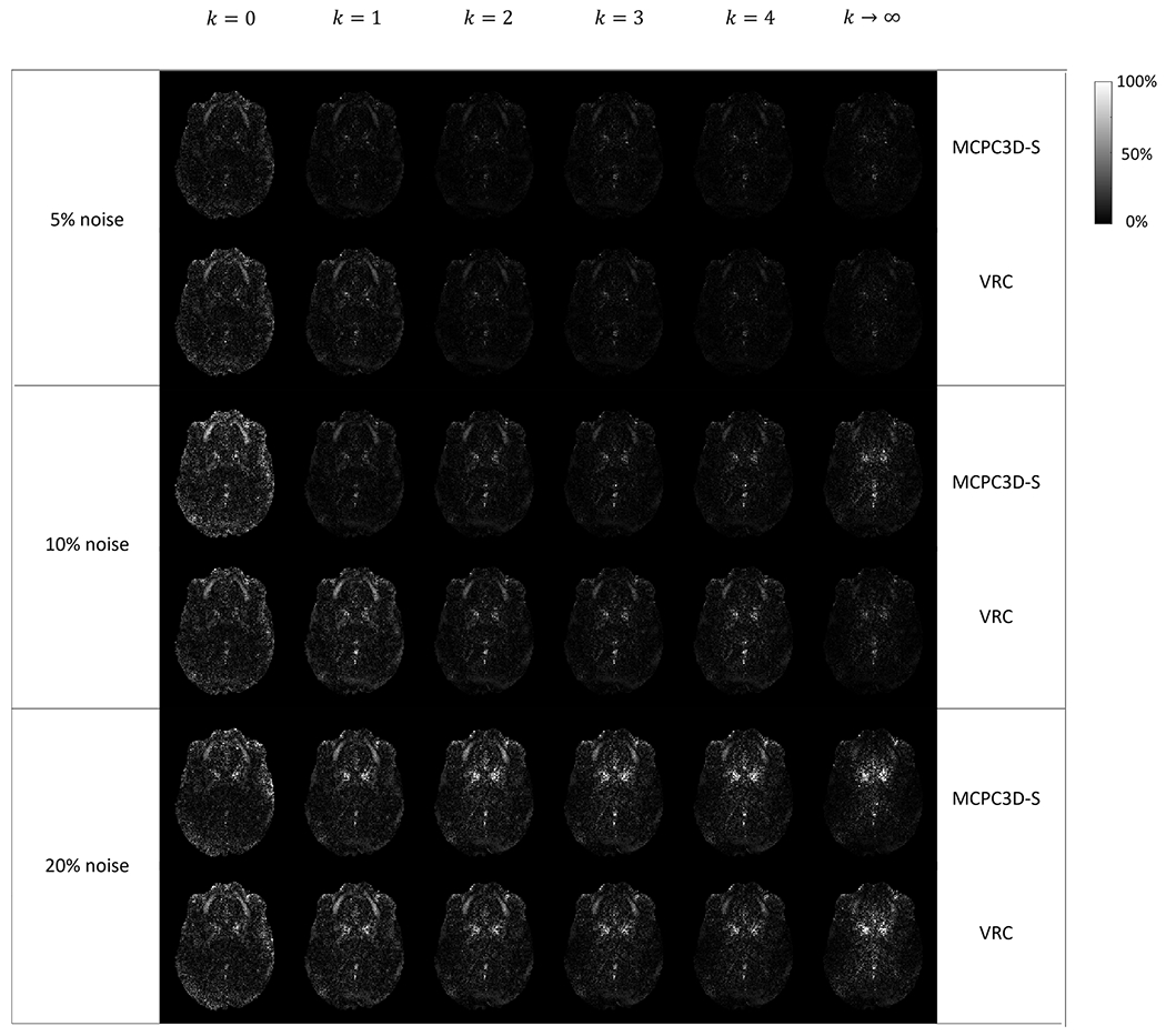
Relative difference (in %) maps between ground truth QSM and QSM maps processed following different phase reconstructions pipelines in the simulated data. Results are shown in one typical axial slice for three different noise levels (5%, 10% and 20%) and considering two phase matching algorithms (MCPC3D-S in the top and VRC in the bottom).
Quantitative analysis shows different behaviors of RMSE by increasing k depending on the analyzed ROI. For ROIs near the location of the coils (Figs. 5.a–d and Sup3.a–d) the RMSE decreases as k increases. However, for central regions (Fig. 5.e and Sup3.e), which were regions far from all coils, the RMSE increases with k. As for the whole brain (Fig. 5.f and Sup3.f) the RMSE showed a minimum at k = 1, and then increased as k increased.
Fig. 5.
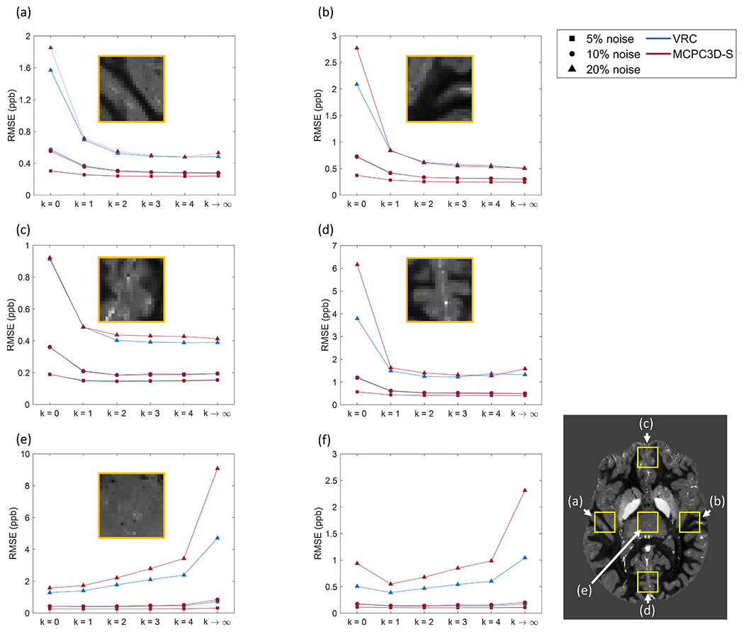
Root-Mean Squared Error (RMSE, in ppb) calculated relative to the ground truth QSM considering different phase reconstruction conditions and three noise levels in the simulated dataset. RMSE was calculated at 5 different ROIs indicated on the map at lower right: (a) right; (b) left; (c) frontal; (d) occipital; (e) central regions, as well as in the whole brain (f). Yellow squares on QSM map show the selected ROIs at each position. Lines in the graphs represent the trending behavior and are indicated for a better visualization. Results are shown for two offset correction methods: VRC (blue) and MCPC3D-S (red); at different noise levels: 5% (■), 10% (●) and 20% (▴).
Comparing the offset correction methods, VRC seemed to show higher relative error at 10% noise level for k = 1 to 4, while it presented lower relative error at k→∞. At 20% noise level no visual difference could be identified regarding the relative difference maps. As for the RMSE, VRC seemed to show lower RMSE when compared to MCPC3D-S at almost all noise levels and regions (Fig. 5 and Sup3). Regardless of the chosen offset correction method, both seemed to show the lowest RMSE at k = 1 overall (Fig. 5.f and Sup3.f).
By comparing the MS from the DGM ROIs of simulated data, both VRC and MCPC3D-S are well correlated to the ground truth even at different k values (R2 > 0.99; p<0.001 for all cases). However, when noise is increased, the angular coefficient of the regression deviates by an amount of around 10% and 13% for VRC and MCPC3D-S, respectively when comparing k = 1 to k = 2 (Fig. 6) and can reach up to 23% and 29% for other values of k.
Fig. 6.
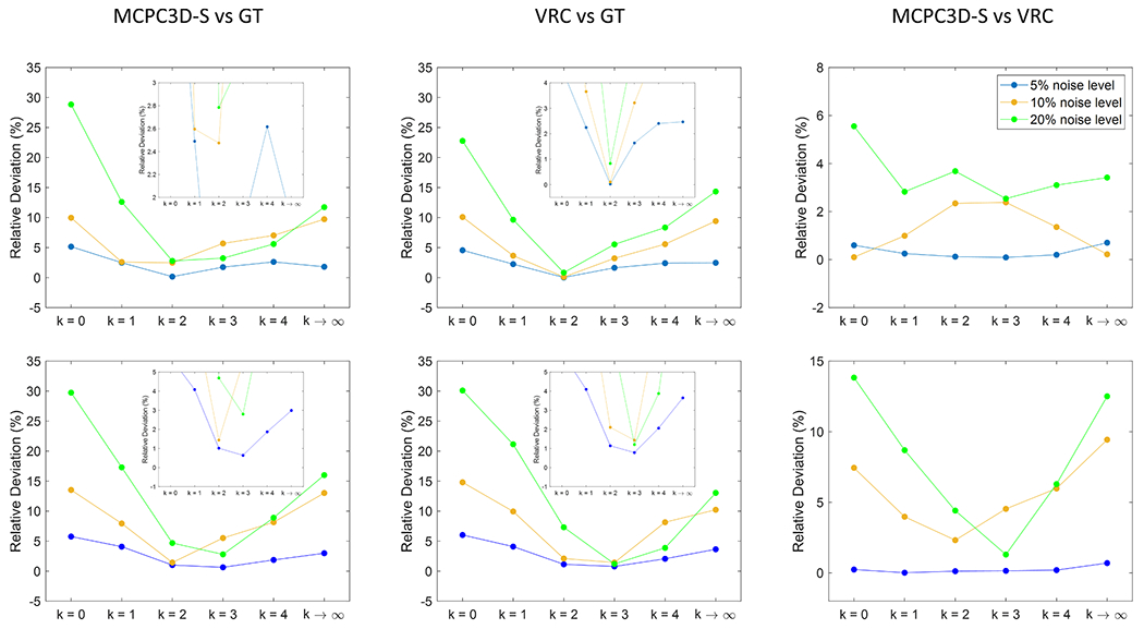
Relative Deviation (in %) in function of k, estimated from the angular coefficient of the linear regression plots at different noise levels.
MCPC3D-S-> phase matching using MCPC3D-S method
VRC -> phase matching using VRC method
GT -> ground truth QSM map
When comparing the susceptibility values between VRC and MCPC3D-S a deviation of 2.8% and 3.7% can be observed, at k = 1 and k = 2, respectively (Fig. 6) and can reach up to 5.6% for other values of k. This deviation increased when increasing the number of coils (Fig. 6), 8.7% and 4.4% at k = 1 and k = 2, respectively, reaching up to 14% for other values of k.
This indicates that k can influence the susceptibility estimation by an amount between 2.6% to 29% depending on the noise level (Fig. 6). However, k seems to have little influence (between 2.5% and 8.7% at the 20% noise level) in the agreement between susceptibility estimated from MCPC3D-S and VRC (Fig. 6).
Postmortem images
Using phase images reconstructed by the scanner with the Adaptive combination resulted on QSM maps with artifacts that compromised the entire map (Fig. 7.a). This happened for a total of 8 subjects (38% of cases) and in all cases presented the same type of artifact (Fig. 7.a).
Fig. 7.
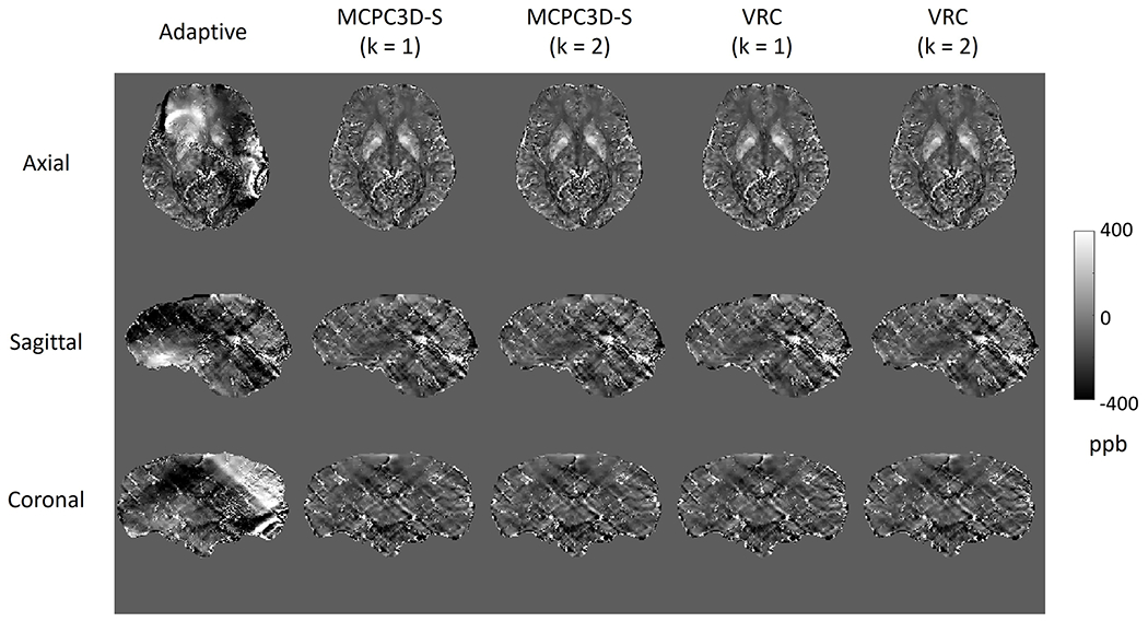
QSM maps generated from the phase images reconstructed by different reconstruction methods for one subject at three different slices orientation.
Adaptive -> Adaptive reconstruction method
MCPC3D-S (k = 1) -> phase matching using MCPC3D-S method and phase combination with k = 1
MCPC3D-S (k = 2) -> phase matching using MCPC3D-S method and phase combination with k = 2
VRC (k = 1) -> phase matching using VRC and phase combination with k = 1
VRC (k = 2) -> phase matching using VRC and phase combination with k = 2
When evaluating the effects of magnitude weighting (k = 1, 2) on MCPC3D-S and VRC corrected QSM maps, it was observed that the MS and SD of selected ROIs had no statistical differences (Figs. 8 and 9). Both offset correction methods and phase combination methods showed high correlation at all evaluated ROIs (R-value between 0.99 and 1.00 with p < 0.01, Fig. 10), except for the Adaptive reconstruction method. Similar result was observed in the Bland-Altman plots (Sup4).
Fig. 8.
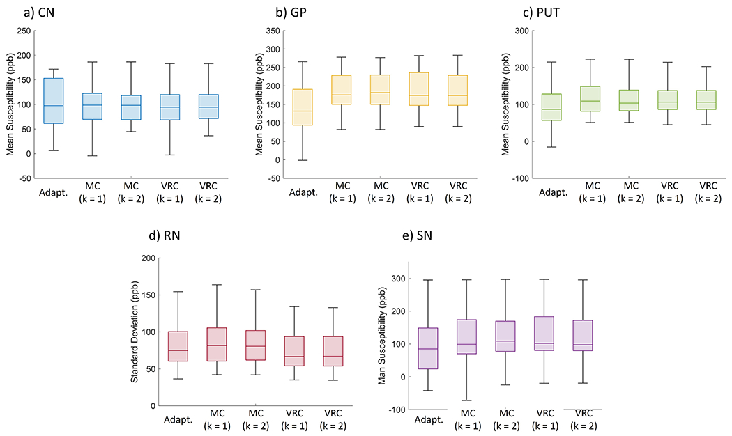
Mean Susceptibility (in ppb) across all subjects for each reconstruction method at five different ROI: a) CN; b) GP; c) PUT; d) RN; e) SN.
Adapt. -> Adaptive method reconstruction.
MC (k = 1) -> phase matching using MCPC3D-S method and phase combination with k = 1.
MC (k = 2) -> phase matching using MCPC3D-S method and phase combination with k = 2.
VRC (k = 1) -> no phase matching and phase combination with k = 1.
VRC (k = 2) -> no phase matching and phase combination with k = 2.
Fig. 9.
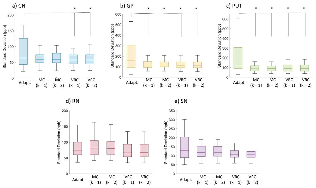
Uniformity (indicated as Standard Deviation in ppb) across all subjects for each reconstruction method at five different ROI: a) CN; b) GP; c) PUT; d) RN; e) SN. Significant differences after ANOVA and t-student tests (p<0.05) are indicated as (*).
Adapt. -> Adaptive method reconstruction.
MC (k = 1) -> phase matching using MCPC3D-S method and phase combination with k = 1.
MC (k = 2) -> phase matching using MCPC3D-S method and phase combination with k = 2.
VRC (k = 1) -> no phase matching and phase combination with k = 1.
VRC (k = 2) -> no phase matching and phase combination with k = 2.
Fig. 10.
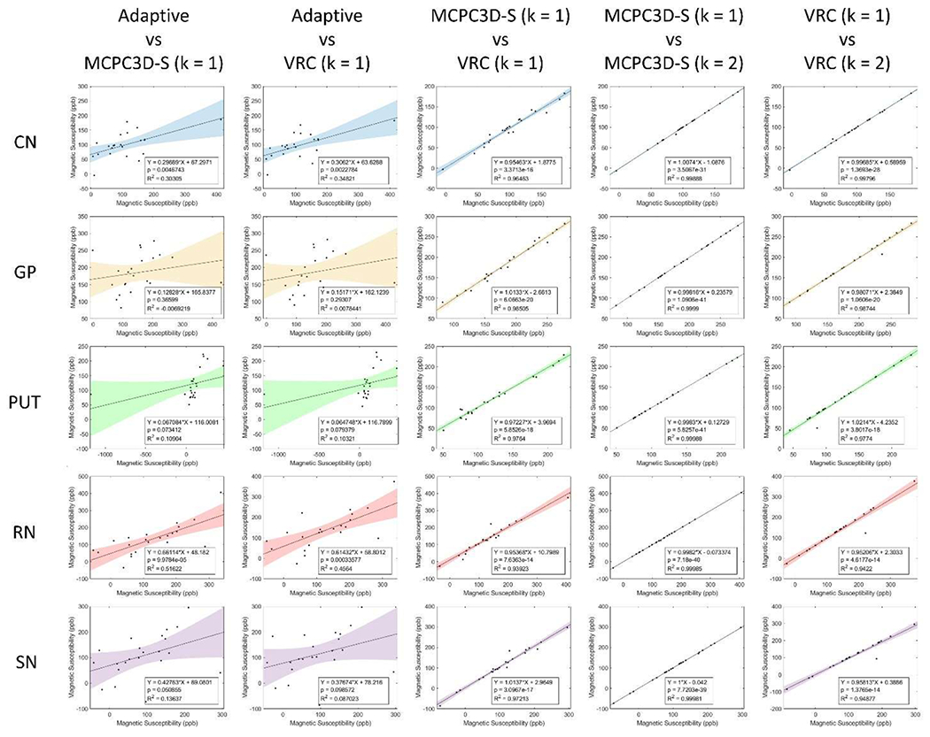
Correlation plots of susceptibility values (in ppb) obtained from QSM images processed from phase data processed by different reconstruction methods. Correlation test (R an p-value) is also indicated for each plot as well as the linear regression.
Discussion
Results from simulated data indicates that combination without weighting factor (k = 0 on Fig. 4, Sup2) downgrades the quality of QSM images. By increasing the power (for k ≥ 1 on Fig. 4), subtle visual differences can only be detected in the low SNR regime (20% noise level, Supl). The RMSE seems to decay with increasing k on regions near the coils (Fig. 5.a–d and Sup3.a–d), while for regions far from the coils (central region) this behavior changes (Fig. 5.e and Sup3.e). Additionally, when evaluating the RMSE over the entire slice, it increased with k (Fig. 5.f and Sup3.f).
Comparison between the offset correction methods showed no visual differences between processed maps, however a closer inspection indicates that the ability to successfully estimate the ground truth susceptibility can be influenced by k up to 29% (Fig. 6) when on high noise regime. Even on appreciable noise levels (10%) the deviation can reach up to 15% (Sup3).
When using higher powers of the weighting factor, the range of optimal SNR region is decreased for each coil, resulting on less coverage of the volume by each coil.
This effect can be seen on Fig. 4 and Fig. 5.e–f (and Sup3.e–f), where the QSM from the k→∞ results on lower SNR and higher RMSE on the central region of the volume. Since this approach simulates a condition of k≫1, by increasing k, a proper combination at central regions of the volume is lost.
Since real data don’t present a ground truth for comparison, quantitative evaluation from postmortem subjects were made with analysis of MS and SD from selected ROIs (Fig. 8 and Fig. 9). The first variable can indicate the similarity between each method in computing the QSM, while the second can be interpreted as an indication of the uniformity of each method (higher SD indicates lower uniformity).
ANOVA test showed no significant differences between both MS and SD when comparing the MCPC3D-S and VRC with k = 1 and k = 2. Significant differences were only observed when comparing each method with the Adaptive method (Fig. 10, first two columns), which indicates that the scanner’s reconstruction algorithm is not optimized for phase images, agreeing with other studies.
QSM maps processed following MCPC3D-S and VRC methods presented a deviation of up to 5.6% (Fig. 10, middle column), which agrees with the simulated data. Additionally, the VRC method seemed to present higher sensitivity to the choice of k, since it presented slightly higher deviation between k values when compared to MCPC3D-S (Fig. 10, last two columns). Taken together with previous results, this seems to indicate that both methods resulted on similar QSM maps, and their difference relative to the ground truth is rather due to the other steps on the reconstruction step of QSM (i.e. phase unwrapping, background field removal and/or dipole inversion).
Although [18] indicated the presence of artifacts in the frontal areas on the MCPC-3D method that arise due to the mask used in the BF step, we did not observe the same effect on our images. It could be due to the BF method here used, since [18] used the V-SHARP method, however [1] also didn’t observe this artifact when using the V-SHARP BF method. Another possibility is that the approach used here to estimate the phase offset was using the MCPC3D-S as demonstrated in [4] which resulted on improved phase images.
Since a reference coil wasn’t available for this study, a complete comparison with other previous studies isn’t possible. [1] showed that methods based on multi-echo resulted on similar results but with slightly higher standard deviation than single-echo methods. Additionally, the authors found that using a virtual reference coil (VRC) resulted on a higher quality QSM maps. In this study we also evaluated both MCPC3D-S and VRC methods in addition to the combination step at different weighting of magnitude. No statistical difference was observed when comparing both methods, and their relative differences only reached up to 5.6% in the scale of ppb. Still, we emphasize that there were some relevant differences between the studies.
QSM maps were processed by using multiples echoes, while Abdulla et al. [1] opted to perform single-echo QSM maps to evaluate the impact of reconstruction methods at different time points. While this could account for nonlinearity effects for the QSM, this can also influence the resulting QSM. Additionally, by implementing a simulated dataset, comparison with ground truth were possible, and analysis on the accuracy of each method were made. Here we observed that both methods suffer from deviations from the ground truth by up to ~20% at low SNR regime, and ~10% at moderate SNR regime and since the difference between each method results on a maximum of 6% even at low SNR regime, these deviations from ground truth must be arising from other steps on QSM processing rather than the phase reconstruction method.
Although the reconstruction methods used in this study did not show significant differences on QSM, it should be noted that each one has different technical limitations and advantages that should be taken into consideration when choosing which method to use.
MCPC3D-S relies on the linear time-evolution of phase assumption. Although it is prone to errors and computational demanding due to the necessity of phase unwrapping, these can be avoided with a proper choice of TEs during the experiment (ASPIRE method). Also, the chosen TE to estimate the offset should be close enough to avoid nonlinear effects to dominate the signal, but far enough to enable sufficient phase evolution. VRC on the other hand can be performed on a single-echo image and is computationally less demanding than the MCPC3D-S. However, it should be noted that the VRI should have enough SNR over the entire volume, and any error on the VRI reconstruction will eventually propagate to the VRC.
There were some limitations to this study. Regarding the postmortem data, due to the acquisition protocol and other issues, other phase matching methods could not be used in this study. Also, the coil combination method used in this study considered magnitude images as an approximation to the signal-to-noise ratio of each coil. For this consideration, we assume an identical gaussian and uncorrelated noise, instead of the real noise profile of each channel. Finally, simplifications were applied to generate the simulated data. While most of these simplifications can be regarded as having little influence on the resulting effects, some of them could have potential influences on the simulations, such as the receiver coil geometry, position, size and quantity. All of these characteristics could change the receiver coil’s coverage of the volume, changing the behavior of resulting maps using different k values. However, it should be noted that our postmortem results agreed to some level to the simulated results.
Conclusion
Our findings indicate that phase offset correction and signal combination are important steps for the QSM processing. Specifically at ultra-high fields, the lack of a reference coil makes it important to look for phase-optimal reconstruction methods over existing methods that comes with commercial scanners. By testing different powers of the magnitude as a weighting factor for the phase sum, no substantial difference could be observed between methods (k ≥ 1). However, according to the simulated data, increasing the power also increases the RMSE of the overall susceptibility map and on central regions of the brain, further decreasing the SNR. On the other hand, the quality of phase maps on cortical regions is improved due to its proximity to the coils. No substantial difference was observed when comparing two different offset correction methods: a multi-echo (MCPC3D-S) and a single-echo (VRC) method. However, when comparing the results of each method to the ground truth on simulated data, a non-negligible difference in the susceptibility estimation was found (up to 20%). This deviation from the ground truth is due to other QSM processing steps, rather than the reconstruction method. As for the choice of a suitable method for phase reconstruction we note that one should look for the pros and cons of each method
Supplementary Material
Acknowledgements
São Paulo Research Foundation (FAPESP, project: 2015/10305–3), Brazilian National Council for Scientific and Technological Development (CNPq, project: 427977/2018–5, project: 142323/2019-5, project: 310618/2021-5 C.E.G.S. fellowship and F.S.O. fellowship), National Institute of Health (NIH) for R01AG070826 grant, and Coordenação de Aperfeiçoamento de Pessoal de Nível Superior – Brasil (CAPES) for financial support. Image Platform at the Autopsy Room (PISA) from the Radiology Institute of the Medical School of University of São Paulo (USP) for the collaboration with acquiring the images.
Footnotes
Declaration of Competing Interest
The authors declare that they have no known competing financial interests or personal relationships that could have appeared to influence the work reported in this paper.
Supplementary materials
Supplementary material associated with this article can be found, in the online version, at doi:10.1016/j.jmro.2023.100097.
Data availability
Data will be made available on request.
References
- [1].Abdulla SU, Reutens D, Bollmann S, Vegh V, MRI phase offset correction method impacts quantitative susceptibility mapping, Magn. Reson.Imaging 74 (2020) 139–151, 10.1016/j.mri.2020.08.009. March. [DOI] [PubMed] [Google Scholar]
- [2].Barbosa JHO, Santos AC, Tumas V, Liu M, Zheng W, Haacke EM, Salmon CEG, Quantifying brain iron deposition in patients with Parkinson’s disease using quantitative susceptibility mapping, R2 and R2*, Magn. Reson. Imaging 33 (5) (2015) 559–565, 10.1016/j.mri.2015.02.021. [DOI] [PubMed] [Google Scholar]
- [3].Chen Z, Johnston LA, Kwon DH, Oh SH, Cho ZH, Egan GF, An optimised framework for reconstructing and processing MR phase images, NeuroImage 49 (2) (2010) 1289–1300, 10.1016/j.neuroimage.2009.09.071. [DOI] [PubMed] [Google Scholar]
- [4].Eckstein K, Dymerska B, Bachrata B, Bogner W, Poljanc K, Trattnig S, Robinson SD, Computationally efficient combination of multi-channel phase data from multi-echo acquisitions (ASPIRE), Magn. Reson. Med (2018), 10.1002/mrm.26963. [DOI] [PubMed] [Google Scholar]
- [5].Haacke EM, Liu S, Buch S, Zheng W, Wu D, Ye Y, Quantitative susceptibility mapping: current status and future directions, Magn. Reson. Imaging (2015), 10.1016/j.mri.2014.09.004. [DOI] [PubMed] [Google Scholar]
- [6].Hammond KE, Lupo JM, Xu D, Metcalf M, Kelley DAC, Pelletier D, Chang SM, Mukherjee P, Vigneron DB, Nelson SJ, Development of a robust method for generating 7.0 T multichannel phase images of the brain with application to normal volunteers and patients with neurological diseases, NeuroImage 39 (4) (2008) 1682–1692, 10.1016/j.neuroimage.2007.10.037. [DOI] [PMC free article] [PubMed] [Google Scholar]
- [7].Langkammer C, Schweser F, Krebs N, Deistung A, Goessler W, Scheurer E, Sommer K, Reishofer G, Yen K, Fazekas F, Ropele S, Reichenbach JR, Quantitative susceptibility mapping (QSM) as a means to measure brain iron? A post mortem validation study, NeuroImage (2012), 10.1016/j-neuroimage.2012.05.049. [DOI] [PMC free article] [PubMed] [Google Scholar]
- [8].Li W, Liu C, Duong TQ, van Zijl PCM, Li X, Susceptibility tensor imaging (STI) of the brain, NMR in Biomed. (2017), 10.1002/nbm.3540. [DOI] [PMC free article] [PubMed] [Google Scholar]
- [9].Li W, Wu B, Avram A.v., Liu C, Magnetic susceptibility anisotropy of human brain in vivo and its molecular underpinnings, NeuroImage 59 (2012) 2088–2097, 10.1016/j.neuroimage.2011.10.038. [DOI] [PMC free article] [PubMed] [Google Scholar]
- [10].Liu C, Susceptibility tensor imaging, Magn. Reson. Med 63 (2010) 1471–1477, 10.1002/mrm.22482. [DOI] [PMC free article] [PubMed] [Google Scholar]
- [11].Liu T, Khalidov I, de Rochefort L, Spincemaille P, Liu J, Tsiouris AJ, Wang Y, A novel background field removal method for MRI using projection onto dipole fields (PDF), NMR in Biomed. 24 (9) (2011) 1129–1136, 10.1002/nbm.1670. [DOI] [PMC free article] [PubMed] [Google Scholar]
- [12].Liu T, Liu J, de Rochefort L, Spincemaille P, Khalidov I, Ledoux JR, Wang Y, Morphology enabled dipole inversion (MEDI) from a single-angle acquisition: comparison with COSMOS in human brain imaging, Magn. Reson. Med 66 (3) (2011) 777–783, 10.1002/mrm.22816. [DOI] [PubMed] [Google Scholar]
- [13].Lu K, Liu TT, Bydder M, Optimal phase difference reconstruction: comparison of two methods, Magn. Reson. Imaging 26 (1) (2008) 142–145, 10.1016/j.mri.2007.04.015. [DOI] [PubMed] [Google Scholar]
- [14].Marques JP, Meineke J, Milovic C, Bilgic B, Chan KS, Hedouin R, van der Zwaag W, Langkammer C, Schweser F, QSM reconstruction challenge 2.0: a realistic in silico head phantom for MRI data simulation and evaluation of susceptibility mapping procedures, Magn. Reson. Med 86 (1) (2021) 526–542, 10.1002/mrm.28716. [DOI] [PMC free article] [PubMed] [Google Scholar]
- [15].Parker DL, Payne A, Todd N, Hadley JR, Phase reconstruction from multiple coil data using a virtual reference coil, Magn. Reson. Med 72 (2) (2014) 563–569, 10.1002/mrm.24932. [DOI] [PMC free article] [PubMed] [Google Scholar]
- [16].Reichenbach JR, Schweser F, Serres B, Deistung A, Quantitative susceptibility mapping: concepts and applications, Clin. Neuroradiol (2015), 10.1007/s00062-015-0432-9. [DOI] [PubMed] [Google Scholar]
- [17].Robinson SD, Bredies K, Khabipova D, Dymerska B, Marques JP, Schweser F, An illustrated comparison of processing methods for MR phase imaging and QSM: combining array coil signals and phase unwrapping, NMR in Biomed. (2017), 10.1002/nbm.3601. [DOI] [PMC free article] [PubMed] [Google Scholar]
- [18].Robinson SD, Dymerska B, Bogner W, Barth M, Zaric O, Goluch S, Grabner G, Deligianni X, Bieri O, Trattnig S, Combining phase images from array coils using a short echo time reference scan (COMPOSER), Magn. Reson. Med 77 (1) (2017) 318–327, 10.1002/mrm.26093. [DOI] [PMC free article] [PubMed] [Google Scholar]
- [19].Roemer PB, Edelstein WA, Hayes CE, Souza SP, Mueller OM, The NMR phased array, Magn. Reson. Med (1990), 10.1002/mrm.1910160203. [DOI] [PubMed] [Google Scholar]
- [20].Vegh V, O’Brien K, Barth M, Reutens DC, Selective channel combination of MRI signal phase, Magn. Reson. Med 76 (5) (2016) 1469–1477, 10.1002/mrm.26057. [DOI] [PubMed] [Google Scholar]
- [21].Wang C, Foxley S, Ansorge O, Bangerter-Christensen S, Chiew M, Leonte A, Menke R, Mollink J, Pallebage-Gamarallage M, Turner MR, Miller KL, Tendler BC, Methods for quantitative susceptibility and R2* mapping in whole postmortem brains at 7T applied to amyotrophic lateral sclerosis, NeuroImage 222 (2020), 10.1016/j.neuroimage.2020.117216. [DOI] [PMC free article] [PubMed] [Google Scholar]
- [22].Wang Y, Liu T, Quantitative susceptibility mapping (QSM): Decoding MRI data for a tissue magnetic biomarker, Magn. Reson. Med (2015), 10.1002/mrm.25358. [DOI] [PMC free article] [PubMed] [Google Scholar]
- [23].Wharton S, Bowtell R, Effects of white matter microstructure on phase and susceptibility maps, Magn. Reson. Med (2015), 10.1002/mrm.25189. [DOI] [PMC free article] [PubMed] [Google Scholar]
- [24].Zheng W, Nichol H, Liu S, Cheng YCN, Haacke EM, Measuring iron in the brain using quantitative susceptibility mapping and X-ray fluorescence imaging, NeuroImage 78 (2013) 68–74, 10.1016/j.neuroimage.2013.04.022. [DOI] [PMC free article] [PubMed] [Google Scholar]
Associated Data
This section collects any data citations, data availability statements, or supplementary materials included in this article.
Supplementary Materials
Data Availability Statement
Data will be made available on request.