Abstract
Accurate and computationally efficient prediction of wave run-up is required to mitigate the impacts of inundation and erosion caused by tides, storm surges, and even tsunami waves. The conventional methods for calculating wave run-up involve physical experiments or numerical modeling. Machine learning methods have recently become a part of wave run-up model development due to their robustness in dealing with large and complex data. In this paper, an extreme gradient boosting (XGBoost)-based machine learning method is introduced for predicting wave run-up on a sloping beach. More than 400 laboratory observations of wave run-up were utilized as training datasets to construct the XGBoost model. The hyperparameter tuning through the grid search approach was performed to obtain an optimized XGBoost model. The performance of the XGBoost method is compared to that of three different machine learning approaches: multiple linear regression (MLR), support vector regression (SVR), and random forest (RF). The validation evaluation results demonstrate that the proposed algorithm outperforms other machine learning approaches in predicting the wave run-up with a correlation coefficient (R2) of 0.98675, a mean absolute percentage error (MAPE) of 6.635%, and a root mean squared error (RMSE) of 0.03902. Compared to empirical formulas, which are often limited to a fixed range of slopes, the XGBoost model is applicable over a broader range of beach slopes and incident wave amplitudes.
-
•
The optimized XGBoost method is a feasible alternative to existing empirical formulas and classical numerical models for predicting wave run-up.
-
•
Hyperparameter tuning is performed using the grid search method, resulting in a highly accurate machine-learning model.
-
•
Our findings indicate that the XGBoost method is more applicable than empirical formulas and more efficient than numerical models.
Keywords: XGBoost, Machine learning, Run-up, Hyperparameter tuning, Grid search method
Method name: XGBoost
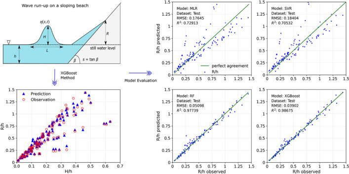
Graphical abstract
Specifications table
| Subject area: | Engineering |
| More specific subject area: | Coastal Engineering |
| Name of your method: | XGBoost |
| Name and reference of original method: | T. Chen and C. Guestrin, “XGBoost: A Scalable Tree Boosting System,” in Proceedings of the 22nd ACM SIGKDD International Conference on Knowledge Discovery and Data Mining, New York, NY, USA, Aug. 2016, pp. 785–794. doi:10.1145/2939672.2939785. |
| Resource availability | N/A |
Introduction
The highest onshore elevation that a wave can achieve measured with respect to the still water level is known as wave run-up. Wave run-up plays an essential role in the increasing area of inundation and can also worsen beach erosion. Since several decades ago, studies related to wave run-up have attracted the interest of many researchers, including researchers in the field of coastal engineering. Run-up studies are crucial in evaluating coastal facilities prior to development. Even yet, it can be challenging to predict the run-up height accurately because it depends on several parameters and also it depends on time and space variables.
When modeling run-up height, including for experimental investigations and calibrating run-up modules in numerical models, solitary waves are often used. On a constant water depth, solitary waves will propagate with constant velocity without changing the waveform. Following Boussinesq [1], the first-order solitary wave solution is as follows
| (1) |
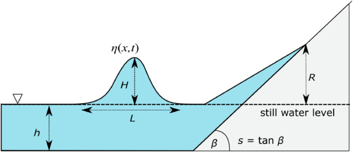
where denotes the height of the solitary wave, the wave number with , and the wave speed with . In this case, the effective wavelength of the solitary wave is , whereas the wave period of the solitary wave is . Here, and denote the undisturbed water depth and the gravity acceleration, respectively. When propagating on a plane beach with slope , this solitary wave will hit the shore and attain a run-up height , see Fig. 1 for an illustration. Numerous researchers propose different but similar formulas for this run-up height . One of the well-known and widely referenced is the run-up empirical formula by Synolakis [2], as follows:
| (2) |
| (3) |
Fig. 1.
An illustration of a solitary wave moving up a gently sloping beach [4].
The recent development of the empirical formulas based on laboratory experiments as a function of beach slope, water depth, and wave amplitude can be found in the literature [3], [4], [5], [6], [7]. However, the applicability and accuracy of these empirical formulas are restricted to specific incident wave amplitudes and coastal slopes [8].
Developing an empirical formula based on laboratory observation data is costly and is limited in some situations. In addition, the derived formula is frequently a simple regression whose accuracy depends on a certain parameter value range. Several researchers worked to address this gap by developing numerical models that could predict the propagation and run-up of solitary waves over a gently sloping beach. Wu and Marsooli [9] utilized a shallow water model to simulate wave run-up on a partly vegetated beach with a sloping shore. Moreover, Adytia et al. [10] developed a Boussinesq model to examine the run-up of solitary waves on a flat sloping beach. In addition, Zhang et al. [11] studied solitary breaking waves using a 3D non-hydrostatic model.
Numerical model-based run-up prediction has several limitations, such as inefficient numerical computation for complex geometries, the need for the numerical scheme to handle run-up phenomena, and the fact that the accuracy of the prediction is highly dependent on the chosen wave model. Although empirical formulas and numerical models have become the standard approach, there has been a trend in recent years to use machine learning methods in developing model predictions. Shen et al. [12] developed real-time prediction based on long short-term memory neural network (LSTM) for the shield moving trajectory during tunneling. They enhanced the LSTM model by employing wavelet transform to reduce irrelevant data noise and the Adam algorithm to optimize the gradient training process of the LSTM. Moreover, Elbaz et al. [13] constructed air quality predictions by integrating a residual network (ResNet) with the convolutional long short-term memory (ConvLSTM). However, there is still little research on run-up models using machine learning in the field of coastal engineering. Abolfathi et al. [8] developed a run-up prediction model by employing a machine learning method based on the Decision Trees algorithm. Yao et al. [14] discussed a multi-layer perceptron neural network to predict the tsunami-like solitary wave run-up over fringing reefs. Rehman et al. [15] recently proposed an artificial neural network (ANN) to predict the maximum wave run-up heights over a series of rubble mounds and caisson-type submerged breakwaters.
As an alternative to the artificial neural network-based deep learning algorithm, we propose the XGBoost method to predict the wave run-up on a sloping beach. XGBoost, which stands for eXtreme Gradient Boosting, is an algorithm for machine learning that was introduced by Chen and Guestrin [16]. XGBoost is an advanced implementation of the gradient boosting algorithm. It is a highly optimized, powerful, and scalable machine-learning algorithm designed for supervised learning problems. Unlike the LSTM algorithm, XGBoost is not an artificial neural network but rather an ensemble of decision trees. Additionally, XGBoost is more efficient in dealing with large datasets and can generate more accurate results since it uses decision trees to identify the most important variables and build models, while artificial neural networks can be computationally expensive and require more training time.
XGBoost is now the most preferred method for developing predictive models due to its remarkable accuracy, efficiency, and adaptability. XGBoost has several advantages compared to other algorithms, such as its ability to handle missing data, highly parallelizable code, and large and complex datasets. Additionally, XGBoost includes several parameters that can be tuned to improve its accuracy further [16]. Furthermore, XGBoost is a robust algorithm for both classification and regression problems. Because of these advantages for model prediction, XGBoost has been increasingly used in ocean and coastal engineering to develop predictive models. Zhang et al. [17] estimated the degree of storm surge disaster losses in coastal regions using an XGBoost-machine learning method. Furthermore, Callens et al. [18] utilized gradient boosting to enhance the wave forecast for a specific area. Recently, Wang et al. [19] developed an XGBoost algorithm to investigate the classification of offshore seabed sediments.
This study aims to develop an XGBoost-based machine learning method to accurately predict run-up for a wide range of coastal slopes and wave amplitudes. As the training dataset for XGBoost, we collected run-up laboratory experiments from several works of literature [2,3,5,6,20]. In addition, the optimal XGBoost model is obtained by hyperparameter tuning. A hyperparameter is a user-specified parameter that influences the training success of a model and, therefore, has a significant effect on the final results of a machine-learning task. The main contributions of this research include: (1) the application of the XGBoost algorithm for the first time to predict wave run-up on sloping beaches accurately, and (2) the ability of the XGBoost method to predict wave run-up not only in various beach slopes but also in a broader range of incident wave amplitude. The present study was one of the first attempts to comprehensively apply the XGBoost method for predicting wave run-up, and it may pave the way for future research on more complex challenges.
Method details
This section describes the XGboost-based machine learning method, including the XGBoost framework, for predicting the wave run-up height.
XGBoost machine learning algorithm
XGBoost is a decision tree-based optimization technique that builds on the gradient descent method. The gradient descent approach is utilized to optimize the loss function, and regularization parameters are employed to prevent overfitting [16]. The fundamental concept of the XGBoost algorithm is to minimize the following objective function, which consists of the loss function and regularization terms [16]:
| (4) |
Here, is the loss function that represents the error between observed data and predicted data , is the model of the t-th tree, and t is the iteration index during the optimization process. The detail of regulation term can be expressed as [16]:
| (5) |
where indicates the total number of tree leaves, and are penalty coefficients, and is a vector containing each leaf's score. More explanations of the XGBoost method can be found in Chen and Guestrin [16].
The parameter in Eq. (5) can be found during the training process; however, several hyperparameters such as , , and must be defined before the training process can begin. Several researchers found that hyperparameter values greatly impact the model accuracy [21]. Therefore, optimal hyperparameters, which may be found by hyperparameter tuning, are required. Grid search, random search, and Bayesian optimization are the three most common methods to optimize hyperparameters. Due to its simplicity, we apply the grid search method in this study.
XGBoost hyperparameter tuning
Table 1 shows some of the most commonly tuned hyperparameters in the XGBoost algorithm. The table also briefly explains each hyperparameter value within its allowed range. In the grid search process, all possible combinations of hyperparameters in the search interval are listed to make grids. Then, utilizing the training dataset, the error resulting from each grid is evaluated via the objective function in Eq. (4). The optimal hyperparameters are those with the lowest error.
Table 1.
Several hyperparameters used in the XGBoost method.
| Hyperparameter | Type | Range | Default | Description |
|---|---|---|---|---|
| colsample_bytree | floating-point | (0, 1] | 1 | The fraction of features that will be utilized to construct each tree |
| learning_rate | floating-point | [0, 1] | 0.3 | Step size at each iteration while the objective function is being optimized |
| max_depth | integer | [0, ∞) | 6 | The maximum depth of each tree; raising this number makes the model more complicated and probably overfit |
| subsample | floating-point | (0, 1] | 1 | The proportion of data that will be sampled for each tree |
| min_child_weight | integer | [0, ∞) | 1 | Minimum instance weight required for a child node |
| n_estimators | integer | [0, ∞) | 100 | The highest number of gradient-boosted trees |
| gamma | floating-point | [0, ∞) | 0 | Minimum loss reduction necessary to create a new partition on a tree leaf node |
| alpha | floating-point | [0, ∞) | 0 | Term for the L2 regularization of weights. Increasing this value will conservatively adjust the model. |
| lambda | floating-point | [0, ∞) | 1 | Term for the L2 regularization of weights. Increasing this value will conservatively adjust the model. |
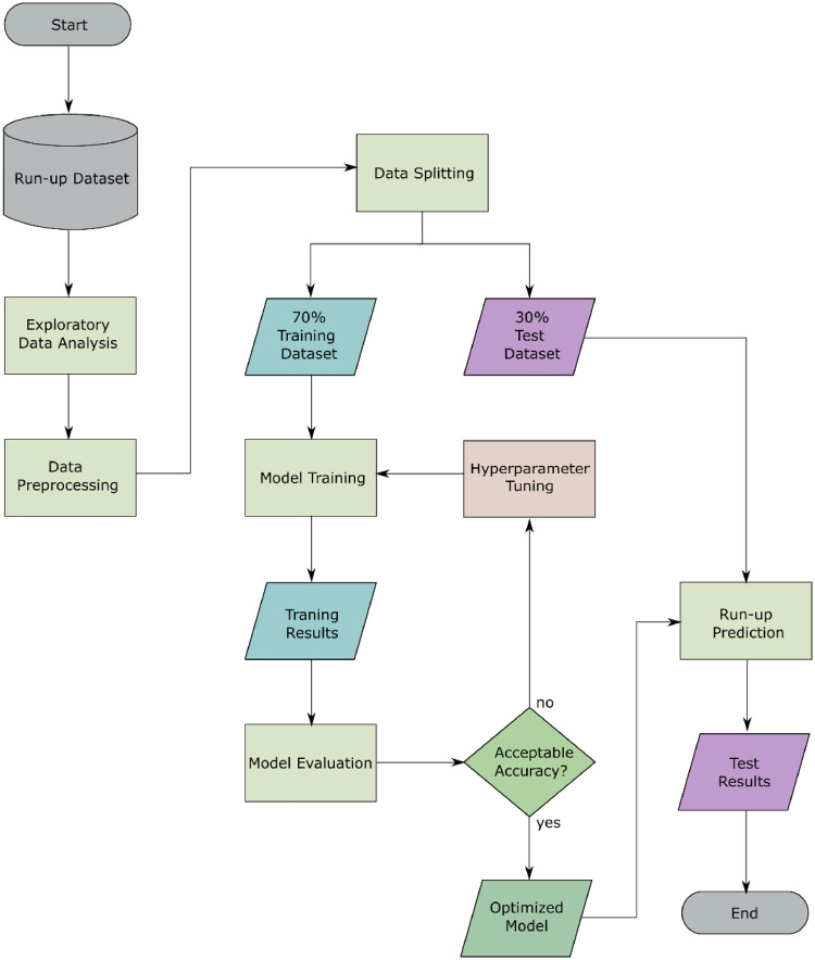
The flowchart of a run-up height prediction model employing the XGBoost-based machine learning approach is depicted in Fig. 2. The procedure can be described as follows:
-
1.
Exploratory data analysis is performed to analyze the pattern of the dataset represented through data visualization.
-
2.
During data preprocessing, missing values and outliers are eliminated.
-
3.
The run-up dataset is split into training and test datasets using specific ratios. The typical ratio is 70% to 30%.
-
4.
Using the XGBoost algorithm, model training is implemented.
-
5.
Utilizing statistical metrics, the XGBoost model training is evaluated. If the desired accuracy is not achieved, hyperparameter tuning is carried out.
-
6.
Hyperparameter tuning is performed using the training dataset. In this study, the grid search method was employed.
-
7.
The XGBoost model is constructed with hyperparameters that have been optimized.
-
8.
The XGBoost model is evaluated by comparing the predicted results to the actual results from the test dataset. This comparison is quantified with statistical measures.
Fig. 2.
XGBoost-based machine learning modeling process for predicting run-up height.
Results and model validation
In this section, we present the XGBoost machine learning approach. This algorithm can predict run-up with high accuracy. The prediction results are then validated with observational data and simulation results from empirical models. However, we will first describe the results of our exploratory data analysis and hyperparameter tuning.
Exploratory data analysis
The dataset employed in this study consists of 439 experimental run-up data. The wave run-up data were collected from literature [2,3,5,6,20]. The run-up data is publicly available and can be obtained directly from the abovementioned literature. The dataset has four features, namely beach slope (s), relative incident wave amplitude (H/h), slope parameter (S0), and type of wave characteristics (type). The label of the dataset is relative run-up (R/h). Here, the slope has a value in the interval [0.017, 1] or the range 1 to 45°. Meanwhile, the type of wave characteristics has a value of SB, PB, and NB, which means surging breaking, plunging breaking, and non-breaking waves, respectively; these values are converted to the integer values of {0,1,2}. The complete statistical results of the run-up dataset are summarized in Table 2, where the mean is the average of the dataset, std is the standard deviation, min and max are minimum and maximum values of the observed data, respectively, and 25, 50, and 75% are 25, 50, and 75th percentiles of the dataset.
Table 2.
The statistical results of the N = 439 observed run-up datasets.
| parameters | mean | std | min | 25% | 50% | 75% | max |
|---|---|---|---|---|---|---|---|
| s | 0.246 | 0.290 | 0.017 | 0.050 | 0.125 | 0.268 | 1.000 |
| H/h | 0.235 | 0.204 | 0.005 | 0.091 | 0.170 | 0.318 | 1.320 |
| S0 | 4.345 | 5.525 | 0.208 | 1.239 | 2.184 | 5.108 | 31.157 |
| type | 1.483 | 0.668 | 0 | 1 | 2 | 2 | 2 |
| R/h | 0.692 | 0.874 | 0.019 | 0.206 | 0.461 | 0.850 | 7.728 |
Fig. 3 shows how the features and labels of the run-up dataset are scattered out and how they relate to each other. The relative run-up, as seen in the figure, lies between 0.02 and 7.73. This run-up dataset may contain outliers. Outliers can significantly impair the performance of a machine-learning model. Removing outliers helps the model to fit the observed data better and make more accurate predictions. Outliers can be calculated by finding the upper and the lower bounds of a normal data range that are 1.5 times the interquartile range below the 75% percentile and above the 25% percentile, respectively. The lower and upper bounds for the relative run-up R/h are 0.019 and 1.60, respectively. Any data point with R/h < 0.019 or R/h > 1.60 is considered an outlier and will be excluded from further investigation. The data trend can also be observed in the figure; as the incident wave amplitude grows, so does the run-up; conversely, as S0 increases, the run-up reduces.
Fig. 3.
Distribution and relationship between variables in the dataset.
The relationship between variables can be seen more clearly in the correlation heat map, which is presented in Fig. 4. A correlation heat map is a type of data visualization commonly displayed as a color-coded matrix with numerical values in each cell. Here, the values in the cells represent the strength of the relationship between each pair of variables. It can be seen from the figure that cells having a positive correlation are colored in shades of blue, and cells with a negative correlation are colored in shades of red. In addition, the darker colors represent stronger relationships. A negative correlation exists when one variable increases while the other decreases, and vice versa. As shown in Fig. 4, it can be easily figured out that the correlation coefficient between the relative amplitude and the relative run-up is 0.89, indicating a very strong correlation between the two variables. However, the remaining three variables have a weak correlation with the relative run-up.
Fig. 4.
Correlation heat map between the input parameters and run-up height.
Measure metric
In this work, the performance of the XGBoost approach in predicting wave run-up is evaluated using the following metrics: mean absolute error (MAE), mean absolute percentage error (MAPE), root mean squared error (RMSE), and correlation coefficient (R2). MAE is the mean absolute difference between the model output (predicted values) and the observations (actual values). MAPE is the average of the absolute percentage deviations between predicted and actual values. RMSE is the square root of the average squared errors between observed and predicted values. R2 measures how closely the predicted values match the actual values. If the R2 value is 1, the predicted values perfectly match the actual values. These statistical error parameters [22,23] can be calculated by
| (6) |
| (7) |
| (8) |
| (9) |
where is the number of observed run-up data, and are the i-th observed and predicted values of run-up, respectively, and is the mean observed value of run-up.
XGBoost implementation
The first step in implementing the XGBoost algorithm is randomly splitting the 439 datasets into training and test data. In most cases, the appropriate ratio for training data to test data is 80:20 or 70:30, where 80% or 70% of the data is used for training, and 20% or 30% is used for testing. However, this ratio can vary depending on the size of the dataset; in this study, the 70:30 ratio was utilized in the implementation of XGBoost. It is worth noting that if the training data is less than 70%, the XGBoost model may be undertrained. This indicates that the developed model may not have enough data to learn from and may therefore be unable to predict the run-up results accurately.
Next, the XGBoost algorithm requires hyperparameters to be set before the training process. These hyperparameters significantly impact the performance of XGBoost. Therefore, we must employ hyperparameter tuning to find the optimal values for the hyperparameters. This study used the grid search method to find the best hyperparameters for the XGBoost. We will focus on optimizing colsample_bytree, learning_rate, max_depth, and subsample, which are the four important hyperparameters, as shown in Table 1. The search range for the selected hyperparameters is detailed in Table 3. It should be noted that the search interval range—the lower and upper bounds of each hyperparameter—is one of the most important steps in hyperparameter tuning since it directly impacts model performance. As discussed in Probst et al. [24], for several hyperparameters, the XGBoost performance is sensitive to small changes in hyperparameter values. In addition, other hyperparameter values were set to their default values. From these search ranges, there are 192 candidates to be evaluated, and by applying 5-fold cross-validation, there are 960 combinations for which the RMSE will be calculated.
Table 3.
The optimal value of hyperparameters tuning.
| Hyperparameter | Search range | Optimal value |
|---|---|---|
| colsample_bytree | [0.5,1] | 1 |
| learning_rate | [0.05,0.35] | 0.15 |
| max_depth | [3,9] | 3 |
| subsample | [0.2,0.6] | 0.6 |
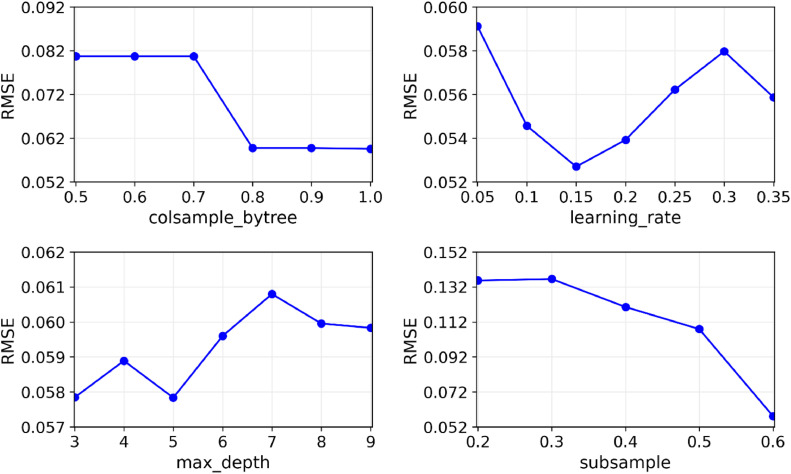
The optimal hyperparameter value is the candidate with the smallest RMSE among all combinations tested. The RMSE results for the four hyperparameters are displayed versus the search range in Fig. 5. The figure shows how the RMSE changes for each hyperparameter; the hyperparameter with the minimum RMSE may be easily found using this figure. Finally, the hyperparameters colsample_bytree, learning_rate, max_depth, and subsample should each be set to 1, 0.15, 3, and 0.6, respectively, for best performance, as listed in Table 3.
Fig. 5.
Relationship between RMSE and some XGBoost hyperparameter optimization results.
XGBoost validation
The performance of the XGBoost model for predicting run-up is evaluated using the test dataset. In addition, the accuracy of the XGBoost is compared to that of three different machine learning methods: multiple linear regression (MLR), support vector regression (SVR), and random forest (RF). MLR is an extension of linear regression, which is used to model the relationship between two or more independent variables and a single dependent variable. SVR is an extension of a support vector machine that uses a subset of training points in the form of support vectors to create a regression model. RF is an ensemble learning technique that integrates number of decision trees to obtain a more precise and stable prediction.
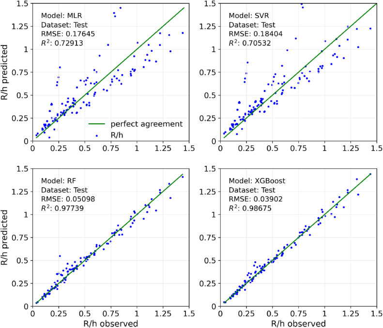
Fig. 6 shows the accuracy of predicted values of the test dataset using XGBoost and other machine-learning approaches. The figure demonstrates that the tree-based models (RF and XGBoost) are fitter than classical machine learning models (MLR and SVR) to predict run-up height on sloping beaches. Given that XGBoost is based on gradient-boosted decision trees, it might be more accurate than the random forest. To gain a more in-depth assessment of each machine learning model's accuracy, we calculate their MAE, MAPE, RMSE, and R2 values.
Fig. 6.
Comparison between observed and predicted run-up for XGBoost and other machine learning meth.
Table 4 summarizes the results of the measure metric calculations for the MLR, SVR, RF, and XGBoost models using the same test data. As seen in the table, the MAE, MAPE, and RMSE of the MLR and SVR models are approximately four times those of the RF and XGBoost models. Furthermore, MLR and SVR have an R2 of 0.7, indicating that they are not accurate enough in predicting run-up height. The test results demonstrate that XGBoost has MAE, MAPE, and RMSE values of 0.02674, 0.06635, and 0.03902, respectively; these values are slightly lower than those of the RF model but much lower than those of the MLR and SVR models. Additionally, the correlation coefficient of XGBoost is 0.98675, indicating that the results predicted by XGBoost closely match the actual results. These statistical errors indicate that XGBoost outperforms other models in forecasting wave run-up on sloping beaches.
Table 4.
MAE, MAPE, RMSE, and R2 values of the XGBoost and other machine learning methods.
| Machine Learning Method | Statistical Measure |
|||
|---|---|---|---|---|
| MAE | MAPE | RMSE | R2 | |
| MLR | 0.12504 | 0.32909 | 0.17645 | 0.72913 |
| SVR | 0.12201 | 0.34558 | 0.18404 | 0.70532 |
| RF | 0.03309 | 0.08799 | 0.05098 | 0.97739 |
| XGBoost | 0.02674 | 0.06635 | 0.03902 | 0.98675 |
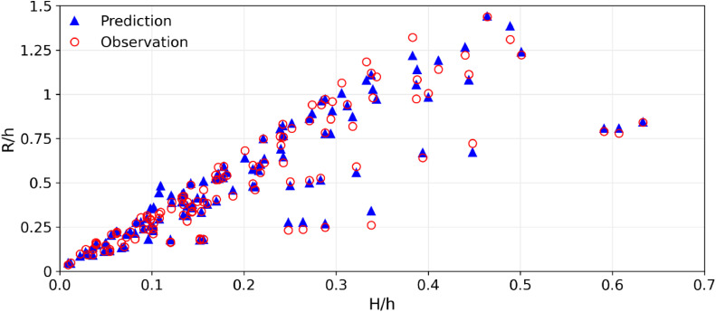
Relative wave amplitude (H/h) is the most important of the four features (H/h, s, S0, and type) in predicting the run-up value (it will be shown at the end of this section). Fig. 7 depicts the predicted run-up values with XGBoost plotted against the wave amplitude. In the figure, the predicted results are compared to observed data (from 30% of test data). The relative amplitude in the interval [0,0.65] will generate the relative run-up in the interval [0,1.5]. The figure shows that XGBoost's run-up predictions agree well with the observed data. This result is consistent with the measurement metric shown in Table 4, which indicates that XGBoost has a correlation coefficient of 0.98675 and a MAPE of 6.635%.
Fig. 7.
Comparison between predicted and observed run-up with respect to wave amplitude.
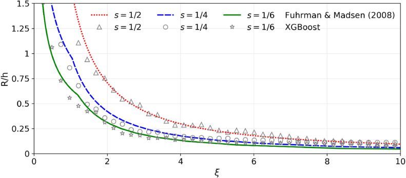
In this section, we also evaluate XGBoost against the empirical formula proposed by Fuhrmann and Madsen [7]. This empirical formula is expressed as follows [4,7]:
| (10) |
where is the surf similarity parameter of solitary waves [7]. The first argument in the minimum function of Eq. (10) is the relative run-up for non-breaking waves, whereas the second argument is for breaking waves. Fig. 8 shows the run-up results predicted by XGBoost and the empirical formula for various slope values (s = 1/2, 1/4, 1/6). In the figure, the relative run-up height (R/h) is plotted against the surf similarity parameter (ξ). As shown in Fig. 8, the XGBoost predictions agree with those of the empirical formula developed by Fuhrman and Madsen [7]. In this assessment, we employ data tests generated from the empirical model to predict run-up results using the developed XGBoost algorithm. As a result, the XGBoost model for predicting run-up height has a wider range of applicability than empirical models, which are often restricted to a specific range of slopes. In addition, the XGBoost is more efficient than conventional numerical models, such as shallow water equations, due to the fact that numerical modeling needs the solution of several complicated partial differential equations with certain numerical methods. Moreover, wave propagation on a sloping beach must be captured in each time step, making the time required to determine the run-up height relatively longer.
Fig. 8.
Run-up results generated by the XGBoost model and empirical model from Fuhrman and Madsen [7] with respect to surf similarity parameters.
Feature importance
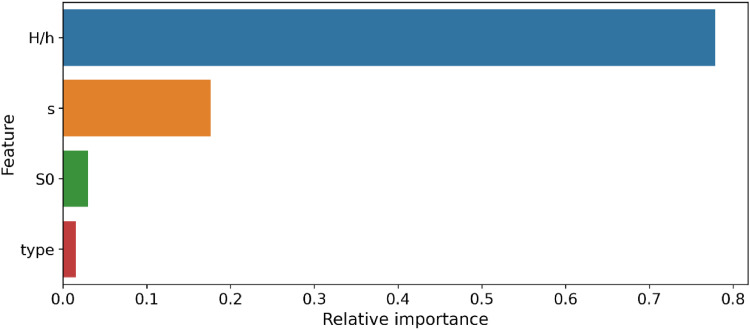
Feature importance measures how much a feature contributes to the target value. For each feature, the higher the score, the more importance will be given to the prediction results. The relative importance of the four features used to predict wave run-up is displayed in Fig. 9. It can be observed from the figure that the incident wave amplitude (H/h) has the most significant relative importance; this indicates that wave amplitude has a more substantial impact on run-up height than other variables. In addition, the slope of the beach (s) is the second most important feature variable.
Fig. 9.
Feature importance ranking.
Conclusion
The XGBoost (eXtreme Gradient Boosting) machine learning algorithm has been developed to predict run-up height as an alternative to empirical formulas and numerical models. XGBoost is an optimization approach based on decision trees and gradient descent. To construct a highly accurate XGBoost model, hyperparameter tuning has been performed using the grid search method. The validation evaluation results show that XGBoost outperforms multiple linear regression (MLR), support vector regression (SVR), and random forest (RF) in predicting wave run-up on sloping beaches, with a correlation coefficient (R2) of 0.98675, a mean absolute error (MAE) of 0.02674, a mean absolute percentage error (MAPE) of 6.635%, and a root mean squared error (RMSE) of 0.03902. Moreover, the XGBoost model has a broader range of applicability than empirical models, which are frequently restricted to a specific slope range. In terms of influence on run-up height, feature importance analysis shows that wave amplitude is more significant than other factors. The XGBoost machine learning approach for run-up prediction offers accuracy comparable to empirical formulas; it can save computing time compared to typical numerical models that must solve several complex partial differential equations.
Ethics statements
Our study used publicly accessible data and did not fulfill the criteria for human subjects research.
CRediT authorship contribution statement
Dede Tarwidi: Conceptualization, Methodology, Validation, Visualization, Formal analysis, Writing – original draft. Sri Redjeki Pudjaprasetya: Supervision, Writing – review & editing. Didit Adytia: Conceptualization, Methodology. Mochamad Apri: Writing – review & editing.
Declaration of Competing Interest
The authors declare that they have no known competing financial interests or personal relationships that could have appeared to influence the work reported in this paper.
Acknowledgments
This research did not receive any specific grant from funding agencies in the public, commercial, or not-for-profit sectors.
Data availability
Data will be made available on request.
References
- 1.Boussinesq J. Théorie des ondes et des remous qui se propagent le long d'un canal rectangulaire horizontal, en communiquant au liquide contenu dans ce canal des vitesses sensiblement pareilles de la surface au fond. J. Mathématiques Pures Appl. 1872:55–108. [Google Scholar]
- 2.Synolakis C.E. The runup of solitary waves. J. Fluid Mech. 1987;185:523–545. doi: 10.1017/S002211208700329X. Dec. [DOI] [Google Scholar]
- 3.Trinaistich W.C., Mulligan R.P., Take W.A. Runup of landslide-generated waves breaking on steep slopes captured using digital imagery and hydrochromic paint. Coast. Eng. 2021;166 doi: 10.1016/j.coastaleng.2021.103888. Jun. [DOI] [Google Scholar]
- 4.Vinodh T.L.C., Tanaka N. A unified runup formula for solitary waves on a plane beach. Ocean Eng. 2020;216 doi: 10.1016/j.oceaneng.2020.108038. Nov. [DOI] [Google Scholar]
- 5.Casella F., Aristodemo F., Filianoti P. A comprehensive analysis of solitary wave run-up at sloping beaches using an extended experimental dataset. Appl. Ocean Res. 2022;126 doi: 10.1016/j.apor.2022.103283. Sep. [DOI] [Google Scholar]
- 6.Hsiao S.C., Hsu T.W., Lin T.C., Chang Y.H. On the evolution and run-up of breaking solitary waves on a mild sloping beach. Coast. Eng. Dec. 2008;55(12):975–988. doi: 10.1016/j.coastaleng.2008.03.002. [DOI] [Google Scholar]
- 7.Fuhrman D.R., Madsen P.A. Surf similarity and solitary wave runup. J. Waterw. Port Coast. Ocean Eng. 2008;134(3):195–198. doi: 10.1061/(ASCE)0733-950X(2008)134:3(195). May. [DOI] [Google Scholar]
- 8.Abolfathi S., Yeganeh-Bakhtiary A., Hamze-Ziabari S.M., Borzooei S. Wave runup prediction using M5′ model tree algorithm. Ocean Eng. 2016;112:76–81. doi: 10.1016/j.oceaneng.2015.12.016. Jan. [DOI] [Google Scholar]
- 9.Wu W., Marsooli R. A depth-averaged 2D shallow water model for breaking and non-breaking long waves affected by rigid vegetation. J. Hydraul. Res. 2012;50(6):558–575. doi: 10.1080/00221686.2012.734534. Dec. [DOI] [Google Scholar]
- 10.Adytia D., Pudjaprasetya S.R., Tarwidi D. Modeling of wave run-up by using staggered grid scheme implementation in 1D Boussinesq model. Comput. Geosci. 2019;23(4):793–811. doi: 10.1007/s10596-019-9821-5. Aug. [DOI] [Google Scholar]
- 11.Zhang J., Liang D., Liu H. An efficient 3D non-hydrostatic model for simulating near-shore breaking waves. Ocean Eng. 2017;140:19–28. doi: 10.1016/j.oceaneng.2017.05.009. Aug. [DOI] [Google Scholar]
- 12.Shen S.L., Elbaz K., Shaban W.M., Zhou A. Real-time prediction of shield moving trajectory during tunnelling. Acta Geotech. 2022;17(4):1533–1549. doi: 10.1007/s11440-022-01461-4. Apr. [DOI] [Google Scholar]
- 13.Elbaz K., Hoteit I., Shaban W.M., Shen S.L. Spatiotemporal air quality forecasting and health risk assessment over smart city of NEOM. Chemosphere. 2023;313 doi: 10.1016/j.chemosphere.2022.137636. Feb. [DOI] [PubMed] [Google Scholar]
- 14.Yao Y., Yang X., Lai S.H., Chin R.J. Predicting tsunami-like solitary wave run-up over fringing reefs using the multi-layer perceptron neural network. Nat. Hazards. 2021;107(1):601–616. doi: 10.1007/s11069-021-04597-w. May. [DOI] [Google Scholar]
- 15.Rehman K., Khan H., Cho Y.S., Hong S.H. Incident wave run-up prediction using the response surface methodology and neural networks. Stoch. Environ. Res. Risk Assess. 2022;36(1):17–32. doi: 10.1007/s00477-021-02076-z. Jan. [DOI] [Google Scholar]
- 16.Chen T., Guestrin C. XGBoost: a scalable tree boosting system. Proceedings of the 22nd ACM SIGKDD International Conference on Knowledge Discovery and Data Mining; New York, NY, USA; 2016. pp. 785–794. Aug. [DOI] [Google Scholar]
- 17.Zhang S., et al. Estimating the grade of storm surge disaster loss in coastal areas of China via machine learning algorithms. Ecol. Indic. 2022;136 doi: 10.1016/j.ecolind.2022.108533. Mar. [DOI] [Google Scholar]
- 18.Callens A., Morichon D., Abadie S., Delpey M., Liquet B. Using Random forest and Gradient boosting trees to improve wave forecast at a specific location. Appl. Ocean Res. 2020;104 doi: 10.1016/j.apor.2020.102339. Nov. [DOI] [Google Scholar]
- 19.Wang F., Yu J., Liu Z., Kong M., Wu Y. Study on offshore seabed sediment classification based on particle size parameters using XGBoost algorithm. Comput. Geosci. 2021;149 doi: 10.1016/j.cageo.2021.104713. Apr. [DOI] [Google Scholar]
- 20.Hall J.V., Watts G.M. US Army Corps of Engineers, Beach Erosion Board; Washington, DC, USA: 1953. Laboratory investigation of the vertical rise of solitary waves on impermeable slopes, Technical Memo Report No. 33. [Google Scholar]
- 21.Zhang W., Wu C., Zhong H., Li Y., Wang L. Prediction of undrained shear strength using extreme gradient boosting and random forest based on Bayesian optimization. Geosci. Front. 2021;12(1):469–477. doi: 10.1016/j.gsf.2020.03.007. Jan. [DOI] [Google Scholar]
- 22.Pan S., Zheng Z., Guo Z., Luo H. An optimized XGBoost method for predicting reservoir porosity using petrophysical logs. J. Pet. Sci. Eng. 2022;208 doi: 10.1016/j.petrol.2021.109520. Jan. [DOI] [Google Scholar]
- 23.Zhu X., Chu J., Wang K., Wu S., Yan W., Chiam K. Prediction of rockhead using a hybrid N-XGBoost machine learning framework. J. Rock Mech. Geotech. Eng. 2021;13(6):1231–1245. doi: 10.1016/j.jrmge.2021.06.012. Dec. [DOI] [Google Scholar]
- 24.Probst P., Boulesteix A.L., Bischl B. Tunability: importance of hyperparameters of machine learning algorithms. J. Mach. Learn. Res. 2019;20(53):1–32. [Google Scholar]
Associated Data
This section collects any data citations, data availability statements, or supplementary materials included in this article.
Data Availability Statement
Data will be made available on request.


