

Abstract
Saddle points are responsible for threshold phenomena of many biological systems. In the heart, saddle points determine the normal excitability and conduction, but are also responsible for certain abnormal action potential behaviors associating with lethal arrhythmias. We investigate the dynamical mechanisms for the genesis of lethal extra heartbeats in heterogeneous cardiac tissue under two diseased conditions. For both conditions, the lethal events occur when the system is close to the saddle point, implying the pivotal role of the saddle point in cardiac arrhythmogenesis.
I. Introduction
A saddle point, an unstable equilibrium of a nonlinear system, is an intersection of a stable and an unstable manifold. Saddle points play important roles in the genesis of complex dynamics in nonlinear systems [1, 2] and are responsible for the threshold phenomena in many physical, chemical, and biological systems [3-5]. In excitable cells [6, 7], such as cardiac and neuronal cells, there is a voltage threshold for excitation. When the stimulus is strong enough to elevate the voltage over the threshold, a positive feedback loop is activated to elicit an action potential. In nerve fibers or cardiac tissue, action potential conduction, whose conduction velocity is also determined by the threshold of excitation, is fundamental for transmission of information in the nerve system or for rhythmic contraction of the heart. Although for an excitable cell, there is only one equilibrium point, the threshold of excitation is determined by the saddle point in the fast subsystem [6, 7]. Therefore, the saddle point plays a key role for life.
In the heart, the electrical excitations originating from the sinoatrial node conduct to the atrium and then to the ventricles to result in normal heart rhythm or sinus rhythm. However, extra systoles, called premature ventricular contractions (PVCs), can occur in the middle of the sinus rhythm, particularly under diseased conditions. Fig. 1(a) shows an electrocardiogram (ECG) from a real patient, in which a PVC occurs in the middle of the sinus rhythm. Unlike the sinus rhythm which originates from the sinoatrial node, a PVC can originate from the Purkinje fibers or anywhere in the ventricles. Clinically, it is widely known that the vast majority of PVCs are benign, but some are linked to lethal ventricular arrhythmias [8-10]. There are many potential mechanisms of PVCs [11], and different mechanisms may occur under different diseased conditions. In long QT syndromes [12-14], it has been postulated that early afterdepolarizations (EADs) are the major cause of PVCs. An EAD [see Fig. 1(b) for an example] is an abnormal depolarization during the repolarization phase of the action potential, which have been widely shown in experiments and computer models. Theoretical analyses [15-17] have shown that EADs begin with a Hopf bifurcation and terminate at a homoclinic bifurcation (HCB) point at which the orbit meets the saddle point. The same bifurcations are also responsible for certain types of bursting behaviors in neurons [18-20] and other cell types [7]. Although EADs are widely considered as a cause of PVCs, and many experimental and computer simulation studies [21-31] have linked EADs to PVCs and focal and reentrant arrhythmias in general, the nonlinear dynamics linking the EADs in a single cell and the genesis of PVCs in tissue remain not well understood. For example, Gray and Huelsing [25] used a two-variable action potential model to show that in the presence of EADs, focal excitations could occur during reentrant arrhythmias while Sato et al [26] used a detailed action potential model to show that multi-focal arrhythmias could occur due to chaos desynchronization. Other simulation studies also showed regional EADs or lengthening of the action potential duration (APD) could result in PVCs, however, the exact condition whether an EAD can cause a PVC or not remains unclear. Here we link the Hopf bifurcation and HCB (or the saddle point) that give rise to EADs in single cells to the PVC genesis in tissue, in particular the critical role of the saddle point. Under another diseased condition called Brugada syndrome, a spike-and-dome action potential behavior is observed and linked to PVCs and lethal arrhythmias [32-36]. We will show in this study that the spike-and-dome phenomenon is also a threshold phenomenon determined by the saddle point. Therefore, the goal of this study is to investigate how the saddle points are linked to the mechanisms of PVC genesis in cardiac tissue. We show that the physiological causes of PVC genesis under these diseased conditions are seemingly different, but they are unified under the same dynamical mechanism that is closely linked to the saddle point.
FIG.1.

PVCs in the heart. (a) An ECG from a real patient with a PVC in the middle of the sinus rhythm. Dots indicate the sinus beats and asterisk indicates the PVC beat. (b) Computer simulation of a 1D cable. Upper panel: Time-space-voltage plot. Magenta is the long APD region which exhibits EADs. Lower panel: Pseudo-ECG. Dots indicate the pacing beats and asterisk indicates the PVC beat. Pacing stimuli are applied at the short APD end (black arrow) with a period of 800 ms. The PVC is induced by lengthening the prior pacing period to 1.4 s. A pacing beat is skipped after the PVC to simulate the skipping of the sinus beat in the real ECG in (a). See Appendix for the parameter setting.
II. Models and Methods
We carry out single-cell and one-dimensional (1D) cable simulations using the 1991 Luo and Rudy (LR1) action potential model [37] with modifications to simulate the diseased conditions. The voltage (V) of the LR1 model is described by the following differential equation: , in which is the stimulus pulse and is the total ionic current density. The ionic currents are functions of V and gating variables which are also described by differential equations. For the 1D cable, V is governed by a partial differential equation, i.e., . D=0.001 ms/cm2 is the diffusion constant. More details of the model and methods are presented in the Appendix.
In this study, we simulated both long QT syndrome and Brugada syndrome. In the case of long QT syndrome, we change the maximum conductance () of [] and the maximum conductance () of []. is an inward current and is an outward current, and thus increasing or decreasing increases APD and promotes EADs. We also change the time constant of the gating variable by multiplying a factor γ, i.e., with γ=6 being the control value. We simulate a 3 cm (or 200 cells with cell length cm) cable. We also simulate a 6 cm cable to investigate the effects of cable length. Repolarization gradient (RG) is induced by altering (by multiplying a factor σ) in one half of the cable, but other ways of setting RG are also used, which will be stated in each case. Fig. 1(b) shows a simulation result of the 1D cable, which recaptures characteristically the ECG behaviors in Fig. 1(a).
In the case of Brugada syndrome, we add a transient outward potassium current () to the model and model the heterogeneity by setting the maximum conductance () differently in each half of the cable. The details are described in Appendix.
III. Results
A. EAD-induced PVCs
To reveal the mechanisms of PVC genesis in the computer model, we first scan and σ for PVCs, shown in Fig. 2(a) as phase diagram. Note that controls the overall APD and σ determines the APD gradient (i.e., RG) in the cable. We pace the cells in the cable simultaneously with a single beat [inset in Fig. 2(a)] so we can compare fairly and accurately the single-cell results with the cable results. The phase diagram exhibits three characteristic structures. In the upper-left region, there is a large PVC region (marked by “RG-PVC”), which is promoted by increasing and/or decreasing σ. A smaller σ corresponds to a longer APD in the long APD region of the cable, resulting in a larger APD gradient. Therefore, the PVCs are potentiated by increasing the RG between the two regions of the cable. Fig. 2(b) shows a PVC from this region.
FIG.2.
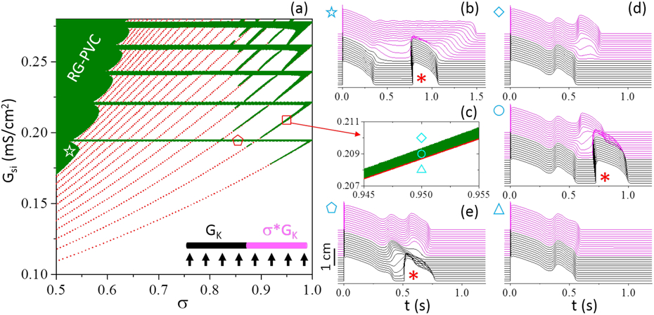
Genesis of PVCs in a 1D cable. (a) Phase diagram showing PVC regions (olive) in σ- space. (b) Time-space-voltage plot for mS/cm2 and σ=0.52 as marked by the star in (a). (c) A blowup view of a small region in the phase diagram marked by the square in (a). (d) Time-space-voltage plots for σ=0.95 and (diamond); 0.209 (circle); and 0.208 (triangle) mS/cm2, respectively, with the same symbols as marked in (c). (e) Time-space-voltage plot for mS/cm2 and σ=0.85 as marked by the pentagon in (a). Red dots in (a) and (c) are the EAD transition points from a single cell with the same parameters as in the long APD region. Inset in (a) is a schematic plot of the cable model. Arrows indicate global pacing. Black and magenta colors mark the short and long APD region, respectively, with the same colors used for voltage in the time-space-voltage plots. In the time-space-voltage plots, the PVC beats are marked by asterisks.
In the upper and upper-right region, there are discretized horizontal bars and tilted belts of PVC regions. The horizontal bars start from the RG-PVC region and end at σ=1. The bars and the belts have a one-to-one relationship and join at σ=1. The red dots are the EAD transition points in a single cell, defined as the parameter point gaining (or losing) an EAD. The single-cell EAD transition points exactly overlap with the lower boundaries of the belts (see Fig. 2 (c) for a blowup view]. The belts are sensitive to both and σ, and are suppressed by decreasing σ. The horizontal bars are sensitive to but independent of α. Above the belt region, there is one more EAD in the long APD region than in the short APD region, but it does not result in a PVC [top panel in Fig. 2(d)]. In the belt region, the EAD results in a PVC [middle panel in Fig. 2(d)]. Below the belt region, the extra EAD in the long APD region disappear. The APD difference becomes small and no PVC occurs [bottom panel in Fig. 2(d)]. The behaviors are similar in the horizontal bars, but the PVC occurs close to the boundary of the cable [Fig. 2(e)]. Because of this, the bars are independent of σ. Note that PVCs cannot occur when σ=1 since the cable becomes homogeneous, and thus σ<1 is still needed to result in a heterogeneity for this type of PVCs. The PVC shown in Fig. 1(b) is caused by the RG mechanism, but the EAD-induced PVCs can also occur under the similar pacing protocol (Fig. 3).
FIG.3.

EAD-induced PVCs under periodic pacing. Pacing stimuli are given at the short APD end indicated by the arrow. Dots indicate the pacing beats and asterisks indicate the PVCs. Upper panel: a time-space-voltage plot. Lower panel: Pseudo-ECG. Pacing cycle length is 960 ms. We use a different and a different from the control, i.e., and mS/cm2. mS/cm2 and σ=6/7.
Both RG and EAD-associated PVCs have been shown in more complex action potential models [27, 28, 31] and experiments [23, 24], but the dynamical mechanisms remain to be elucidated. To understand the mechanistic link between EADs in single cells and PVCs in tissue, and the causes of the discretized narrow bars and belts in the phase diagram, we first show how the HCB affects the PVC genesis. In the previous study [15], using a fast-slow system analysis approach [7, 18, 38], we showed that the EAD originates from a Hopf bifurcation and terminates at the HCB in the fast subsystem. Here we show that the transition point shown in Fig ,2(a) is when the EAD takes off right at the HCB point, which is shown in Fig. 4. In the LR1 model, X is the variable that has the largest time constant which is much larger than the time constants of other variables [39]. Moreover, to facilitate the observation of EADs, we slow it further by multiplying a factor γ to as mentioned above in methods. Therefore, X is used as the slow variable in the fast-slow analyses. In the fast-slow system analyses, since the slow variable changes much slower than other variables, one treats the slow variable as a parameter and investigates the bifurcations in the fast subsystem with respect to the slow variable. Fig. 4(a) shows the bifurcation diagram of the fast subsystem with X being treated as a parameter. We also plot three trajectories from a single cell with different γ values. These γ values are the same as those marked by the symbols in Fig. 4(b). Note that since γ only alters the time constant of the slow variable X, it does not affect the bifurcations of the fast subsystem. Therefore, changing γ only change the trajectory of the whole system but not the bifurcation diagram of the fast subsystem shown in Fig. 4(a). Fig. 4(b) is a small phase diagram in the σ-γ plane, showing a very narrow PVC region above the EAD transition points [similar to Fig. 2(c)]. Fig. 4(c) shows three voltage plots from the phase diagram marked by the symbols in Fig. 4(b), which are the same as for the three trajectories in Fig. 4(a). As shown in Fig. 4(a), when γ=5.95 (blue), the action potential has one EAD and the voltage just passes beyond the HCB point, leading to repolarization. When γ=6 (red), X grows slightly slower, and at the end of the first EAD, the system is still within the HCB point, and thus a second EAD forms. When γ=6.05 (olive), the second EAD takes off at an X value even further away from the HCB point, and the EAD amplitude becomes slightly smaller. Note that PVCs only occur for γ=6, not for γ=5.95 or γ=6.05. Therefore, PVCs tend to occur when the last EAD of the cell (in the long APD region) takes off at the vicinity of the HCB point (or just above the saddle point).
FIG.4.

Instabilities promoting PVCs. (a) Bifurcation diagram of the fast subsystem in which the slow variable X is treated as a parameter. Black solid and dashed lines are the stable and unstable steady states of the fast subsystem, respectively. The green lines are the maximum and minimum voltage of the oscillations of the fast subsystem. The lower branch of the green lines meets the saddle point at the homoclinic bifurcation (HCB). The other colored lines are the trajectories of the whole system with σ=0.95 and three different γ values: γ=5.95 (blue), γ=6 (red), and γ=6.05 (olive). The lower panel is a blowup view of the region close to the homoclinic bifurcation point as marked by the box in (a). (b) A small phase diagram in σ-γ space. Red dots are the EAD transition points of the single cell. (c) Time-space-voltage plots for the same σ and γ values as in (a) with symbols marked in (b). Asterisk marks the PVC beat. (d) Time and space plots of ΔV (color scaled) for different γ values as marked. PVCs occur for γ=6 but not for other γ values shown.
To gain more insights into the mechanism of PVC genesis, we calculate the spatiotemporal evolution of a perturbation to the spatiotemporal solution (see Appendix) and plot the voltage component (ΔV) in Fig. 4(d) for different γ values between 5.95 and 6.05 (PVCs occur for γ between 5.985 and 6.015). As γ increases from 5.95 to 5.985 (bottom-up arrow), ΔV grows at the long APD side prior to the occurrence of a new EAD in the long APD side. On the other hand, for γ from 6.05 to 6.015 (top-down arrow), ΔV grows in the gradient region (i.e., the middle region), indicating that a spatial instability occurs to result in a PVC. Therefore, the all-or-none EAD behavior (cellular instability) causes a sudden increase of RG in the middle region, resulting in a spatial instability for the genesis of PVCs. However, this instability is suppressed when the EAD takes off further away from the HCB point.
The reason that we choose to change γ in Fig. 4 instead of or σ is that changing γ does not affect the bifurcations of the fast subsystem but alters the EAD takeoff position [Fig. 4(a)]. Because of this property. it is more convenient and clearer to demonstrate the link between the saddle point and the genesis of PVCs. On the other hand, changing or σ will change both the bifurcation diagram of the fast subsystem and the EAD’s takeoff position. However, only when the EAD takeoff position is close to the saddle (HCB) point, PVC can occur, which can only be satisfied with certain and σ values, giving rise to the narrow belts in the phase diagram [Fig. 2(a)].
In the cases shown in Figs.1-4, we use a 3 cm (200-cell) cable and a sudden change in in the middle of the cable. To show the effects of a graduate change in , we linearly decrease from the large value to the small value over 100 cells (see inset in Fig. 5). Fig. 5 shows the phase diagram. Comparing Fig. 5 to Fig. 2(a), the graduate change in results in the following changes. The RG-PVC region is reduced. At the joints of bars and belts, the PVC regions are increased, i.e., the corners of these joints are filled with data points of PVCs. In other words, the gradual change in in space can promote EAD induced PVCs. This can be understood as follows. For a sudden change in , decreasing σ quickly increases RG, and increasing RG tends to suppress PVCs as shown in Fig. 4. For a graduate change in , decreasing σ has a smaller effect on increasing RG, and thus for the same σ value, PVCs can occur more easily in the case of gradually changing in space. However, as σ becomes large, there is almost no difference between the two types of heterogeneities. Note that there is no change in the positions of the bars and belts, and the belts still overlap with the single-cell EAD transition lines.
FIG.5.

Phase diagram showing PVC regions (olive) in a cable with graduate change in in the middle 100 cells of the cable (inset). The phase diagram is plotted the same way as Fig. 2(a).
We also carry out simulations in a longer cable. Fig. 6 shows the phase diagram obtained from a 6 cm (400-cell) cable in which the short APD region is 1.5 cm and the long APD region is 4.5 cm [inset in Fig. 6(a)]. Comparing Fig. 6(a) to Fig. 2(a), one can see that there are no other changes from Fig. 2(a) except that the belts are extended to much smaller α values. To show how this occurs, we plot some examples of PVCs in Fig. 6(b) for parameters from the locations marked by the symbols in the phase diagram in Fig. 6(a). For an σ value close to one (diamond), the RG is small, a PVC arises close to the border of the short and long APD regions. As σ decreases (circle and triangle), the PVC arises from the long APD region, being more and more distant away from the border region. This can be understood as follows. As σ decreases, the APD in the long APD region becomes longer, increasing RG in the border region. However, the RG decreases gradually away from the border region, and thus there will be always a location where the RG is mild enough for the EAD to induce a PVC. Therefore, decreasing σ causes the PVC to originate further away from the border region. Note that only the last EAD in the long APD region gives rise to a PVC, agreeing with the fact that only the EAD taking off from the saddle (or HCB) point can result in a PVC. Other EADs fails to induce PVCs. Also note that in the previous [31], we showed that decreasing the diffusion constant extends the belts to smaller σ values without other changes to the phase diagram, which is equivalent to increasing the cable length.
FIG.6.

PVC behaviors in a 6 cm cable. (a) phase diagram plotted the same way as Fig. 2(a). (b) Time-space-voltage plots for the three locations in phase diagram as marked by the symbols in (a). mS/cm2. σ=0.953 (diamond), σ=0.879 (circle), and σ=0.78 (triangle).
B. Spike-and-dome action potential morphology induced PVCs
Besides EADs, another type of action potential behavior, called spike-and-dome phenomenon, can also lead to PVCs, occurring under the diseased condition called Brugada syndrome [32-34]. In this case, the spike-and-dome action potential behavior is promoted by an ionic current called . We added an formulation [40] to the LR1 model (see Appendix). Fig. 7(a) shows action potentials for different maximum conductance . As increases, the spike-and-dome morphology enhances and once is increased to a critical value, the action potential suddenly loses the dome, resulting in a spike-like short action potential [the transition point is marked by the arrow in Fig. 7(a)]. We plot the bifurcation of the fast subsystem and the trajectories as in Fig. 4(a), showing that the transition point is also the saddle point of the fast subsystem [Fig. 7(b)].
FIG.7.

Spike-and-dome morphology and PVCs induced by . (a) APs with mS/cm2 and (black), 0.5 (red); 1.03255 (blue), 1.0326 (green), and 1.5 (olive) mS/cm2. The transition point is between the blue and green traces as marked by the arrow. (b) Steady states in the fast subsystem with mS/cm2 (black solid and dotted lines) with X being the slow variable, and the trajectories for action potentials in (a) with the same colors. (c) Phase diagram showing the PVC region (olive) and the single-cell transition points (red dots). Inset is a schematic plot of the cable model. (d) Time-space-voltage plots for mS/cm2 and different as marked (unit: mS/cm2). Asterisk marks the PVC beat. (e) Time and space plots of ΔV (in color scale) for different values as marked. A PVC occurs for mS/cm2 but not for other values shown.
We then carry out 1D cable simulations with presence in one-half of the cable to induce PVCs [see inset in Fig. 7(c)]. We scan and for PVCs, shown as a phase diagram in Fig. 7(c). Similar to the EAD case, PVCs only occur in a narrow region below the spike-and-dome transition point when and are large enough. Fig. 7(d) shows three examples of time-space-voltage plot above, inside, and below the PVC region, respectively. We also calculate the evolution of a perturbation to the spatiotemporal solution with ΔV shown in Fig. 7(e). As decreases from large to small toward the PVC region (top-down arrow), ΔV grows in the short APD side, which eventually leads to the transition from the spike-and-dome to the spike morphology. As increases from small to large toward the PVC region (bottom-up arrow), ΔV grows in the gradient region (middle of the cable). Therefore, the same instabilities as for the EAD case occur to result in PVCs. The difference is that in the EAD case, multiple bars and belts of PVC regions can exist in the phase diagram while in the case, only one belt exists. Another difference is that in the EAD case, PVCs occur when the long APD region gains an EAD and the PVC region is above the transition point, while in the case, the PVC region is below the transition point since PVCs occur when the short APD region loses the dome.
We also carry out simulations using two fixed values in the cable to generate action potential heterogeneities and scan and for PVCs. Fig. 8(a) shows the phase diagram for mS/cm2 in the first half and mS/cm2 in the second half of the cable. The red dots are the transition points from spike-and-dome to spike in the single cell for mS/cm2 and purple for mS/cm2. PVCs only occur very close to the transition points of the large . Increasing in the two regions of the cable promotes PVCs (Fig. 8b), i.e., PVCs occur in a much wider region between the two transition lines. Note that above the red line APD is long with a spike-and-dome morphology in the whole cable and below the purple line APD is short with a spike morphology in the whole cable. In both regions, no PVC can occur. PVCs can only occur between the two transition boundaries.
FIG.8.

Phase diagrams showing the PVC regions (olive) and the single-cell transition points (red and purple dots). The red dots are the transition points for the higher value and the purple dots for the lower value in the cable (as indicated in the insets). (a) mS/cm2 in the first half of the cable and mS/cm2 in the second half. (b) mS/cm2 in the first half and mS/cm2 in the second half of the cable. APD is long in whole cable above the red line and short in the whole cable below purple line.
IV. Conclusions
In summary, we investigate the dynamical mechanisms of PVC genesis under two diseased conditions: long QT syndrome and Brugada syndrome. Although the physiological causes and cellular dynamics are seemly different, the dynamical mechanisms of PVC genesis are the same. In other words, for both conditions, an all-or-none behavior resulted from the saddle-point dynamics causes a sudden increase of RG, which then causes a tissue-scale instability responsible for PVC genesis. However, when the system is further away from the saddle point, PVCs are suppressed by the RG, leading to narrow PVC regions in the phase diagrams. Moreover, the all-or-none behavior caused by the saddle-point dynamics promotes chaos [15, 41], which can further potentiate the genesis of PVCs via chaos desynchronization [30]. Therefore, the saddle points not only are important for the normal heart rhythm but also can lead to lethal arrhythmias. Since some types of neural bursting are caused by the same bifurcations as for EADs in cardiac cells [18-20], the insights from this study may also be helpful for understanding the conduction of neural bursting in the nerve system.
Acknowledgements
This work was supported by National Institutes of Health grants R01 HL134709 and R01 HL139829.
Appendix
1. Mathematical models
We used the 1991 Luo and Rudy (LR1) action potential model [37] with modifications to simulate the diseased conditions in this study. Here we give a brief description of the differential equations of the original LR1 model and our modifications to the model. For details of the formulations, please go to the original publication [37].
The membrane voltage () is described by the following differential equation:
| (A1) |
where is the membrane capacitance. is the stimulus current density, which is a 2 ms duration and −30 μA/cm2 pulse. is the total ionic current density consisting of different types of ionic currents, i.e.,
| (A2) |
where is the Na+ current; is called the slow inward current, which is known as the L-type Ca2+ current; , , and are K+ currents; and is the background current. , , and are functions of voltage. , , and are functions of both voltage and gating variables, with the following formulations:
| (A3) |
| (A4) |
| (A5) |
where m, h, j, d, f and X are gating variables described by the following type of differential equation:
| (A6) |
where and are functions of . , , and are parameters called maximum conductance. , , and are reversal potentials. We set and thus the differential equation for [Ca2+]i was dropped since it becomes independent. Therefore, the model becomes a 7-variable model.
For the 1D cable, the governing partial differential equation for is:
| (A7) |
where cm2/ms. We simulated a 3 cm long cable discretized to 200 cells ( cm).
For simulating the EAD-induced PVCs, we made the following changes to the parameters of the model: ; ; ; mS/cm2; and mS/cm2. Heterogeneities in the 1D cable were simulated by multiplying a factor σ (<1) to in the long APD region [as indicated in Fig. 2(a)].
For the simulation shown in Fig. 1(b), we used a different , i.e., and a different , i.e., mS/cm2 to better match the real ECG in Fig. 1(a). We used mS/cm2 and σ=0.2 for Fig. 1(b).
For the spike-and-dome action potential morphology induced PVCs, we added an to the total ionic current, i.e.,
| (A8) |
with formulated as [40]:
| (A9) |
where and are the gating variables satisfying the same type of differential equation as Eq. (A6). With the addition, the single cell model is a now 9-variable model. We used the original parameters of the LR1 model with mS/cm2 as control. Heterogeneities in the 1D cable were simulated by setting differently in the two halves of the cable while other parameters are uniform in the whole cable.
2. Initial conditions
We gave a single stimulus at t=0 with a fixed initial condition. For simulations of the EAD case, the initial condition was set as: V=−78.9 mV, m=0.005, h=0.95, j=0.95, d=0.005, f=0.99995, and X=0.09. For the simulations of the case, the same values of the above variables were used together with and .
3. Calculating the evolution of a perturbation in the cable
We calculated the evolution of a perturbation to the spatiotemporal solution in the cable using the linearized equations from Eq. (A7). For the EAD case, the linearized equations are:
| (A10) |
where is the Jacobian and is the vector composed of all the variables of the cable model, i.e.,
FIG.9.

Time and space plots of evolution of the perturbation (indicated by color scales) to the other variables for the case of γ=6.015 shown in Fig. 4(d).
| (A11) |
is the spatial index of the cells in the cable. is the vector of perturbation to the variables, i.e.,
| (A12) |
Since the length of the 1D cable contains 200 cells, then is a (7 * 200) × (7 * 200) matrix. In the simulations shown in this study, we only simulate a single beat with a fixed initial condition. To allow the initial perturbation to evolve into the eigendirection (or a steady state) of the tangent space, such as in the calculation of the largest Lyapunov exponent, we repeated the calculation for many beats. Specifically, we took the spatiotemporal solution from 0 to 2 s and repeated this for many periods. At the beginning of each period, we rescaled the vector. The reason that we did not pace the system with a period of 2 s (or other periods) is because under periodic pacing, complex dynamics can easily occur [15, 41], and thus we cannot maintain the system at a periodically steady state. Fig. 9 shows the time-space color plots for the evolution of the perturbation to the other 6 variables for the case of γ=6.015 shown in Fig. 4(d).
We did the same simulations for the case with and added to calculate the evolution of the perturbation in the tangent space.
Since we rescaled the vectors every period, the scale of ΔV shown in Fig. 4 and Fig. 7 is only relative.
4. Calculation of Pseudo-ECG
The pseudo-ECG was calculated as:
| (A13) |
where and is a point in the cable and (xp,yp)=(1.5 cm, 1 cm) is the location of the pseudo-ECG electrode.
5. Numerical methods
An explicit Euler method for the differential equations of voltage and the Rush-Larsen method [42] for the equations of the gating variables were used to numerical integration with a fixed time step Δt = 0.01 ms. For the 1D cable, cm was used. No-flux boundary conditions were used. All the codes were programed in CUDA C++, and simulations were performed on NVIDIA Tesla K80 GPU cards (NVIDIA, Santa Clara, CA).
References
- [1].Guckenheimer J, and Holmes P, Nonlinear oscillations, dynamical systems, and bifurcations of vector fields (Springer-Verlag, New York, 1983). [Google Scholar]
- [2].Ott E, Chaos in Dynamical Systems (Cambridge Unversity Press, New York, 2002). [Google Scholar]
- [3].Gardner TS, Cantor CR, and Collins JJ, Construction of a genetic toggle switch in Escherichia coli, Nature 403, 339 (2000). [DOI] [PubMed] [Google Scholar]
- [4].Xiong W, and Ferrell JE Jr., A positive-feedback-based bistable 'memory module' that governs a cell fate decision, Nature 426, 460 (2003). [DOI] [PubMed] [Google Scholar]
- [5].Tyson JJ, Chen KC, and Novak B, Sniffers, buzzers, toggles and blinkers: dynamics of regulatory and signaling pathways in the cell, Curr. Opin. Cell Biol 15, 221 (2003). [DOI] [PubMed] [Google Scholar]
- [6].Fitzhugh R, Thresholds and Plateaus in the Hodgkin-Huxley Nerve Equations, The Journal of General Physiology 43, 867 (1960). [DOI] [PMC free article] [PubMed] [Google Scholar]
- [7].Keener JP, and Sneyd J, Mathematical Physiology (Springer, New York, 1998), p. 766. [Google Scholar]
- [8].Ruberman W, Weinblatt E, Goldberg JD, Frank CW, and Shapiro S, Ventricular premature beats and mortality after myocardial infarction, N. Engl. J. Med 297, 750 (1977). [DOI] [PubMed] [Google Scholar]
- [9].Kennedy HL, Whitlock JA, Sprague MK, Kennedy LJ, Buckingham TA, and Goldberg RJ, Long-term follow-up of asymptomatic healthy subjects with frequent and complex ventricular ectopy, N. Engl. J. Med 312, 193 (1985). [DOI] [PubMed] [Google Scholar]
- [10].Glass L, Multistable spatiotemporal patterns of cardiac activity, Proc Natl Acad Sci U S A 102, 10409 (2005). [DOI] [PMC free article] [PubMed] [Google Scholar]
- [11].Qu Z, and Weiss JN, Mechanisms of Ventricular Arrhythmias: From Molecular Fluctuations to Electrical Turbulence, Annu. Rev. Physiol 77, 29 (2015). [DOI] [PMC free article] [PubMed] [Google Scholar]
- [12].Morita H, Wu J, and Zipes DP, The QT syndromes: long and short, The Lancet 372, 750 (2008). [DOI] [PubMed] [Google Scholar]
- [13].Lerma C, Lee CF, Glass L, and Goldberger AL, The rule of bigeminy revisited: analysis in sudden cardiac death syndrome, J. Electrocardiol 40, 78 (2007). [DOI] [PubMed] [Google Scholar]
- [14].Clancy CE, and Rudy Y, Linking a genetic defect to its cellular phenotype in a cardiac arrhythmia, Nature 400, 566 (1999). [DOI] [PubMed] [Google Scholar]
- [15].Tran DX, Sato D, Yochelis A, Weiss JN, Garfinkel A, and Qu Z, Bifurcation and Chaos in a Model of Cardiac Early Afterdepolarizations, Phys. Rev. Lett 102, 258103 (2009). [DOI] [PMC free article] [PubMed] [Google Scholar]
- [16].Kügler P, Early afterdepolarizations with growing amplitudes via delayed subcritical Hopf bifurcations and unstable manifolds of saddle foci in cardiac action potential dynamics, PLoS ONE 11, e0151178 (2016). [DOI] [PMC free article] [PubMed] [Google Scholar]
- [17].Huang X, Song Z, and Qu Z, Determinants of early afterdepolarization properties in ventricular myocyte models, PLOS Computational Biology 14, e1006382 (2018). [DOI] [PMC free article] [PubMed] [Google Scholar]
- [18].Shilnikov A, Calabrese RL, and Cymbalyuk G, Mechanism of bistability: tonic spiking and bursting in a neuron model, Phys Rev E Stat Nonlin Soft Matter Phys 71, 056214 (2005). [DOI] [PubMed] [Google Scholar]
- [19].Channell P, Cymbalyuk G, and Shilnikov A, Origin of bursting through homoclinic spike adding in a neuron model, Phys. Rev. Lett 98, 134101 (2007). [DOI] [PubMed] [Google Scholar]
- [20].Del Negro CA, Hsiao CF, Chandler SH, and Garfinkel A, Evidence for a novel bursting mechanism in rodent trigeminal neurons, Biophys. J 75, 174 (1998). [DOI] [PMC free article] [PubMed] [Google Scholar]
- [21].Yan G-X, Wu Y, Liu T, Wang J, Marinchak RA, and Kowey PR, Phase 2 Early Afterdepolarization as a Trigger of Polymorphic Ventricular Tachycardia in Acquired Long-QT Syndrome: Direct Evidence From Intracellular Recordings in the Intact Left Ventricular Wall, Circulation 103, 2851 (2001). [DOI] [PubMed] [Google Scholar]
- [22].Choi BR, Burton F, and Salama G, Cytosolic Ca2+ triggers early afterdepolarizations and Torsade de Pointes in rabbit hearts with type 2 long QT syndrome, J Physiol-London 543, 615 (2002). [DOI] [PMC free article] [PubMed] [Google Scholar]
- [23].Maruyama M et al. , Genesis of phase 3 early afterdepolarizations and triggered activity in acquired long-QT syndrome, Circ Arrhythm Electrophysiol 4, 103 (2011). [DOI] [PMC free article] [PubMed] [Google Scholar]
- [24].Liu J, and Laurita KR, The mechanism of pause-induced torsade de pointes in long QT syndrome, J. Cardiovasc. Electrophysiol 16, 981 (2005). [DOI] [PubMed] [Google Scholar]
- [25].Gray RA, and Huelsing DJ, Excito-oscillatory dynamics as a mechanism of ventricular fibrillation, Heart Rhythm 5, 575 (2008). [DOI] [PMC free article] [PubMed] [Google Scholar]
- [26].Sato D, Xie LH, Sovari AA, Tran DX, Morita N, Xie F, Karagueuzian H, Garfinkel A, Weiss JN, and Qu Z, Synchronization of chaotic early afterdepolarizations in the genesis of cardiac arrhythmias, Proc Natl Acad Sci U S A 106, 2983 (2009). [DOI] [PMC free article] [PubMed] [Google Scholar]
- [27].Huang X, Kim TY, Koren G, Choi B-R, and Qu Z, Spontaneous initiation of premature ventricular complexes and arrhythmias in type 2 long QT syndrome, American Journal of Physiology - Heart and Circulatory Physiology 311, H1470 (2016). [DOI] [PMC free article] [PubMed] [Google Scholar]
- [28].Vandersickel N, de Boer TP, Vos MA, and Panfilov AV, Perpetuation of torsade de pointes in heterogeneous hearts: competing foci or re-entry?, The Journal of Physiology 594, 6865 (2016). [DOI] [PMC free article] [PubMed] [Google Scholar]
- [29].Dutta S, Mincholé A, Zacur E, Quinn TA, Taggart P, and Rodriguez B, Early afterdepolarizations promote transmural reentry in ischemic human ventricles with reduced repolarization reserve, Prog. Biophys. Mol. Biol 120, 236 (2016). [DOI] [PMC free article] [PubMed] [Google Scholar]
- [30].Liu W, Kim TY, Huang X, Liu MB, Koren G, Choi BR, and Qu Z, Mechanisms linking T-wave alternans to spontaneous initiation of ventricular arrhythmias in rabbit models of long QT syndrome, The Journal of Physiology 596, 1341 (2018). [DOI] [PMC free article] [PubMed] [Google Scholar]
- [31].Zhang Z, Liu MB, Huang X, Song Z, and Qu Z, Mechanisms of premature ventricular complexes caused by QT prolongation, Biophys. J 120, 352 (2021). [DOI] [PMC free article] [PubMed] [Google Scholar]
- [32].Antzelevitch C, and Yan G-X, J-wave syndromes: Brugada and early repolarization syndromes, Heart Rhythm 12, 1852 (2015). [DOI] [PMC free article] [PubMed] [Google Scholar]
- [33].Cantalapiedra IR, Penaranda A, Mont L, Brugada J, and Echebarria B, Reexcitation mechanisms in epicardial tissue: role of I(to) density heterogeneities and I(Na) inactivation kinetics, J. Theor. Biol 259, 850 (2009). [DOI] [PubMed] [Google Scholar]
- [34].Maoz A, Krogh-Madsen T, and Christini DJ, Instability in action potential morphology underlies phase 2 reentry: a mathematical modeling study, Heart Rhythm 6, 813 (2009). [DOI] [PubMed] [Google Scholar]
- [35].Maoz A, Christini DJ, and Krogh-Madsen T, Dependence of phase-2 reentry and repolarization dispersion on epicardial and transmural ionic heterogeneity: a simulation study, Europace 16, 458 (2014). [DOI] [PMC free article] [PubMed] [Google Scholar]
- [36].Bueno-Orovio A, Cherry EM, Evans SJ, and Fenton FH, Basis for the Induction of Tissue-Level Phase-2 Reentry as a Repolarization Disorder in the Brugada Syndrome, BioMed Research International 2015, 12 (2015). [DOI] [PMC free article] [PubMed] [Google Scholar]
- [37].Luo CH, and Rudy Y, A model of the ventricular cardiac action potential: depolarization, repolarization, and their interaction, Circ. Res 68, 1501 (1991). [DOI] [PubMed] [Google Scholar]
- [38].Izhikevich EM, Dynamical Systems in Neuroscience (MIT press, Cambridge, 2007). [Google Scholar]
- [39].Landaw J, and Qu Z, Memory-induced nonlinear dynamics of excitation in cardiac diseases, Phys. Rev. E 97, 042414 (2018). [DOI] [PMC free article] [PubMed] [Google Scholar]
- [40].Dumaine R, Towbin JA, Brugada P, Vatta M, Nesterenko DV, Nesterenko VV, Brugada J, Brugada R, and Antzelevitch C, Ionic Mechanisms Responsible for the Electrocardiographic Phenotype of the Brugada Syndrome Are Temperature Dependent, Circ. Res 85, 803 (1999). [DOI] [PubMed] [Google Scholar]
- [41].Landaw J, Garfinkel A, Weiss JN, and Qu Z, Memory-Induced Chaos in Cardiac Excitation, Phys. Rev. Lett 118, 138101 (2017). [DOI] [PMC free article] [PubMed] [Google Scholar]
- [42].Rush S, and Larsen H, A practical algorithm for solving dynamic membrane equations, IEEE Trans. Biomed. Eng 25, 389 (1978). [DOI] [PubMed] [Google Scholar]