Protocol for performing pooled CRISPR-Cas9 loss-of-function screens

Summary

Phenotypic screens involving pooled CRISPR-Cas9 libraries offer a powerful, rapid yet affordable approach to evaluate gene functions on a global scale. Here, we present a protocol for performing pooled CRISPR-Cas9 loss-of-function screens to identify genetic modifiers using either fluorescence-based or cell death phenotypic readouts. We describe steps for designing and amplifying the library and generating and screening cells. We then detail deep sequencing and statistical analysis using cas9 High Throughput maximum Likelihood Estimator.

For complete details on the use and execution of this protocol, please refer to Bersuker et al. (2019),¹ Li et al. (2022),² and Roberts et al. (2022).³

Graphical abstract

Highlights

• •Detailed instructions for pooled CRISPR-Cas9 screen design
• •Identify genetic modifiers using cell-death-based and fluorescence-based readouts
• •Detailed steps for deep sequencing and statistical analysis using casTLE

Publisher’s note: Undertaking any experimental protocol requires adherence to local institutional guidelines for laboratory safety and ethics.

Phenotypic screens involving pooled CRISPR-Cas9 libraries offer a powerful, rapid yet affordable approach to evaluate gene functions on a global scale. Here, we present a protocol for performing pooled CRISPR-Cas9 loss-of-function screens to identify genetic modifiers using either fluorescence-based or cell death phenotypic readouts. We describe steps for designing and amplifying the library and generating and screening cells. We then detail deep sequencing and statistical analysis using cas9 High Throughput maximum Likelihood Estimator.

Before you begin

Genetic screens are powerful, unbiased discovery approaches to systematically elucidate the genes involved in a process or phenotype of interest. With the emergence of CRISPR-Cas9 genome editing tools, the multitude of readily available single guide RNA (sgRNA) libraries, and the improved accessibility of CRISPR screen analysis pipelines, genetic screens in mammalian cells are rapidly becoming an indispensable staple of cell biology research. These screens include both loss-of-function, CRISPR knockout (KO) and CRISPR interference (CRISPRi), and gain-of-function, CRISPR activation (CRISPRa), screens. In a typical pooled CRISPR screen, an sgRNA plasmid library is introduced using viral based transduction into pools of cells expressing the appropriate Cas9 version – Cas9 for CRISPR KO, dCas9 fused to a transcriptional repressor for CRISPRi, and dCas9 fused to a transcriptional activator for CRISPRa. Cells expressing unique sgRNAs are then selected based upon a phenotype of interest, such as altered viability following a treatment or a change in the levels of a fluorescent reporter. The sgRNAs that influence the phenotype are then identified by deep sequencing and bioinformatics programs that quantify sgRNA enrichment between controls and treatments.

We have performed death-based and fluorescence-activated cell sorting (FACS)-based CRISPR KO screens to identify key regulators of ferroptosis^1,2 and lipid droplet biology,³ respectively. The methods employed in our studies are generalizable and can be readily employed to address a myriad of cell biology questions that provide selectable phenotypes. Here, we provide a step-by-step protocol for designing, performing, and analyzing pooled CRISPR KO screens in mammalian cells using either cell viability or fluorescent reporters as selection methods (Figure 1).

Figure 1.

Schematic illustrating the major protocol steps for pooled CRISPR screens

Experiments

Generate Cas9-expressing cells

Timing: 4 weeks

The CRISPR-Cas9 system includes two main parts: the Cas9 endonuclease and targeting sgRNAs. Both components can be introduced together or separately through lentiviral transduction. This integrates Cas9 and sgRNAs non-specifically into the genome, which is appropriate for almost all CRISPR screens in immortalized cells. However, if Cas9 needs to be expressed more specifically, such as when using stem cells, it can be expressed from a safe harbor locus.⁴ In this protocol, we induce constitutive Cas9 expression through lentiviral transduction. Cas9 is then stably expressed and remains active throughout the screening process.

• 1.Plate 300,000 HEK293T cells into one well of a 6-well culture plate in 1 mL DMEM + 10% FBS such that they are at ∼50% confluence 24 h later.
• 2.After 24 h, transfect HEK293T cells with Mirus LT1 transfection reagent, 500 ng 3rd generation lentiviral packaging vector mix (equal parts pMDLg/pRRE [Addgene # 12251], pRSV-Rev [Addgene # 12253], and pMV2.g [Addgene # 12259]), and 500 ng pLenti-Cas9-blast (Addgene # 52962) at a 3:1 Mirus:DNA ratio. Follow Mirus Bio’s “TransIT-LT1 Full Transfection Protocol” (link).

CRITICAL: To ensure sufficient viral titers are reached, all library and packaging plasmids should be endotoxin-free and the packaging HEK293T cells need to be healthy prior to transfection.

• 3.Incubate cells for 72 h.
• 4.After 72 h, collect viral supernatant through a 0.45 μm filter. Use immediately or store at 4°C for up to one week or −80°C for up to six months.

CRITICAL: When working with lentivirus, bleach all media and supplies and turn on ultraviolet light in the biosafety cabinet for thirty minutes to inactivate viral particles.

• 5.Plate 100,000 HuH7 cells into two wells of a 6-well tissue culture plate in DMEM + 10% FBS such that cells are at ∼80% confluence 24 h later.
• 6.After 24 h, introduce 0.5 mL fresh DMEM + 10% FBS and 0.5 mL pLenti-Cas9-blast lentivirus-containing medium to the cells in one well with 8 μg/mL polybrene. Incubate for 24 h.

Note: Keep one well uninfected as a control for the antibiotic selection.

• 7.
  After 24 h, remove viral media and replace with DMEM + 10% FBS.

  • a.
    Expand cells for 24 h and then begin antibiotic selection with 4 μg/mL blasticidin.

    Note: With the amount of lentivirus added in step 6, ∼30%–50% of cells should be infected. Cells can therefore start selection at high confluency and not overgrow the plate.

  • b.
    Replace the selection media every 3–4 days and split cells as necessary until all control cells have died.

    Note: The concentration of selection antibiotic is dependent on the cell line. This concentration should be determined in advance with antibiotic kill curves.

• 8.Once all control cells have died, replace media for Cas9 cells with fresh DMEM + 10% FBS without antibiotic to allow cells to recover. These are now your “Cas9” cells.

Note: Cas9 pools or clonal cells can be used for CRISPR screening. To avoid clonal bias from the genetic background, we screen pools of Cas9 cells and do not select monoclonal cells.

• 9.Validate Cas9 expression by Western blot (Figure 2A).
• 10.Freeze cells at −80°C and store in liquid nitrogen.

Note: It is useful to expand these cells and store in excess since they can be used for subsequent screens or individual gene knockouts.

Note: After introduction into cells, it is important to make sure that Cas9 is active (steps 11-16). To test Cas9 activity, independently infect cells with a lentiviral plasmid encoding: 1. mCherry plus a non-targeting sgRNA (control) and 2. mCherry plus an mCherry-targeting sgRNA (Figure 2B). Employ flow cytometry to measure mCherry expression (Figure 2C). Cells expressing active Cas9 will cleave the mCherry DNA and appear as an mCherry negative population. Conversely, cells lacking active Cas9 will fail to cleave the mCherry DNA and appear as an mCherry positive population. Due to the long half-life of mCherry, it may take up to 1–2 weeks to distinguish the active Cas9 (e.g., mCherry-negative) cells.

• 11.Repeat steps 1–4 to make lentiviral media containing a control sgRNA or mCherry-targeting sgRNA (see key resources table for sequences) cloned into pMCB320 lentiviral vector (Addgene # 89359).
• 12.Plate 100,000 HuH7 Cas9 cells into three wells of a 6-well plate in DMEM + 10% FBS so that cells reach ∼80% confluence 24 h later.
• 13.After 24 h, introduce viral media containing the control sgRNA or the mCherry-targeting sgRNA cloned into the pMCB320 lentiviral vector with 8 μg/mL polybrene to two of the wells. Incubate for 24 h.

Note: Keep one well uninfected for antibiotic selection.

• 14.After 24 h, remove viral media and replace with DMEM + 10% FBS. Expand cells for 48 h and then begin antibiotic selection with 2 μg/mL puromycin (see note above on antibiotic concentrations). Replace the selection media every 3–4 days until all control cells have died.
• 15.Once all control cells have died, replace media with fresh DMEM + 10% FBS without antibiotics to allow cells to recover.
• 16.Measure mCherry fluorescence by flow cytometry to validate Cas9 activity (Figures 2B and 2C).

Figure 2.

Generation of Cas9 stable-expressing cell line

(A) Representative western blot showing the expression of Cas9 in cells.

(B) Schematic of the mCherry self-cutting system to evaluate Cas9 activity.

(C) Example of analyzing Cas9 activity with the mCherry self-cutting system. HuH7 cells were infected with lentivirus expressing either sgmCherry or sgNone and selected by puromycin for one week. mCherry expression in cells was examined by flow cytometry.

Dose response analysis to determine concentration of cytotoxic compounds

Timing: 3–4 days

An optimal concentration of your choice compound to induce cell death is crucial to achieving the maximum dynamic range of the screen readout. For a drug-resistance screen, we suggest determining a sub-lethal concentration of drug that causes very modest cell death (∼5%) in 24-48 h. Presumably, the depletion of a drug resistance factor will lead to a substantial increase in the sensitivity to the drug (Figures 3A and 3B), leading to a depletion of the sgRNA over time. For a drug-sensitivity screen, we recommend an initial drug concentration that causes ∼50% cell death. However, as pools of surviving cells from the initial selection will become resistant to cell death induced by the drug, a slightly higher concentration may be required for each subsequent treatment cycle to achieve ∼50% death.

Note: This is a specific example for identifying ferroptosis resistance factors using known ferroptosis inducing compounds. However, this protocol can be extrapolated to any treatment or condition that provides a selective pressure on cell viability.

Note: HuH7 and U-2 OS cells were used in our original studies,^2,3 and the data used to generate Figures 3A and 3B were collected from U-2 OS cells. However, the protocol steps to test dose-response cytotoxicity can be applied to any cell type.

• 17.On day 0, seed ∼5,000 U-2 OS cells in each well of a 96-well plate such that the final volume per well is 200 μL.
• 18.On day 1, aspirate the media from the 96 well-plate and replace it with 100 μL fresh media.
• 19.Prepare a 2× final solution of the compound at varying concentrations by serial dilution in media containing 60 nM SYTOX Green Dead Cell Stain.

Note: 8–12 different concentrations are recommended to ensure that the optimum concentration is within the standard curve. We usually begin with a 10-point, 5-fold dilution series.

• 20.Slowly add 100 μL compound containing media back to each well so that the final volume of media in each well is 200 μL with 30 nM SYTOX Green Dead Cell Stain.
• 21.Monitor cell death using an Incucyte Live-Cell Analysis System (Essen Biosciences), taking images every 2 h for 24–48 h total. Dead cells will be SYTOX green-positive.
• 22.On day 2 or 3, determine the percentage of cell death by dividing the number of dead cells (SYTOX green-positive) by the total number of cells (visualized by phase imaging).

Note: Due to some limitations of the Incucyte system and the dramatic difference in cell morphology, thresholding and automatically counting total cell number using phase images can sometimes be difficult and inaccurate. Generating a cell line that stably expresses mCherry or using a genetically encoded live-cell nuclear marker (e.g., Incucyte Nuclight reagents) greatly improves the accuracy of the counting for live cells.

Note: If an Incucyte Live-Cell Analysis System is not available, a CellTiter-Glo 2.0 Cell Viability Assay can be used to determine the sub-lethal dose of the drug.

• 23.Choose a concentration of drug that results in ∼5% cell death. Use this concentration for the CRISPR screen (Figures 3A and 3B).

Figure 3.

Determination of selection strategy for pooled CRISPR screens

(A and B) Characterization of sub-lethal dose of the desired compound for the treatment of cells by IncuCyte (A) or Cell-titer Glo 2.0 assay (B). Shading indicates 95% confidence intervals for the fitted curved and each data point is the average of three replicates. AUC, Area Under the Curve.

(C) Example of dynamic range of cell populations measured by flow cytometry strategy to optimize the dynamic range of a FACS-based screen.

Determine the dynamic range for fluorescence-based assays

Timing: 1 week

The confidence of screen results depends on the dynamic range of the fluorescence reporter. A greater distance between the high and low fluorescence intensity bins will result in less biological noise and will increase the confidence of positive results and reduce the occurrence of false positives and negatives.⁵ When possible, it is useful to determine the dynamic range of a cell population using a positive control prior to screening to ensure that cells with altered phenotypes can be accurately sorted by FACS.

Note: Fluorescence can arise from a fluorescent reporter protein or a fluorescent dye. To obtain the highest dynamic range from a reporter protein, it may be useful to sort cells to obtain a population with uniform fluorescence levels. For fluorescent dyes, test multiple concentrations and incubation times.

Note: It is important to establish the timeframe and treatment conditions before performing the screen itself. For example, it may take several days for a genetic perturbation or drug to produce a measurable effect on a fluorescent reporter. Cells may also need to be differentiated or pretreated with drugs or nutrients. Therefore, optimize conditions and establish a timeline for seeding cells, inducing genetic perturbations, differentiating (if applicable), and treating cells, and carry it over to the screen to yield the most robust results.

• 24.Choose a positive control gene (if possible) that is known to influence levels of the fluorescent reporter. Generate a knockout cell line or treat cells with a drug targeting the positive control protein. Confirm that the expected increase or decrease in fluorescence is detectable by flow cytometry
• 25.
  Measure fluorescence by flow cytometry to validate that a change in fluorescence is detected and to determine the dynamic range of your assay (Figure 3C).

  • a.
    In this example, HuH7 cells were treated with 1 μg/mL triacsin C or 100 μM oleic acid to deplete or increase neutral lipid storage, respectively. Cells were treated with 1 μg/mL BODIPY 493/503 to label netral lipids and fluorescence was measured by flow cytometry. The 10× decrease and 5× increase in fluorescence intensity will be the target dynamic range of fluorescence for this CRISPR screen.

Note: Fluorescence intensity can diminish over time. Incubate cells on ice for multiple hours (as long as the FACS sort will be) and check that fluorescence does not change during sorting. We have not found this to be an issue with GFP-based reporters. If necessary, cells can be fixed prior to FACS to ensure fluorescent marker stability over time.

Note: In some cases, there are no drugs or known regulators to manipulate or validate the system. In the absence of a positive control to validate the fluorescence reporter, it is possible to move directly to the screen.

Prepare sgRNA library

Timing: 3 days

Many genome-scale and small-scale libraries are deposited on Addgene. For our experiments, we used the Bassik Human CRISPR Knockout Library (Addgene # 101926-101934), which is composed of 9 sublibraries, or our custom Human Lipid Droplet and Metabolism Library (Addgene # 191535). Each sgRNA library will need to be amplified and packaged into lentivirus. Alternatively, pre-packaged lentivirus can be purchased directly from Addgene.

Note: Certain biological questions may require genome-wide screens, and others may be more accurately addressed using specialized libraries based on gene function. The number and availability of resources (e.g., cell culture supplies, equipment booking, etc.) also differs drastically between a genome-wide screen and a smaller custom library-based screen. Additionally, CRISPR libraries from different sources may contain a different number of sgRNAs per gene or may work by delivering multiple sgRNAs to individual cells (e.g., one sgRNA on a single plasmid vs. multiple sgRNAs on a single plasmid), which can be a consideration when calculating the amount of time needed to complete a screen. For more information on this subject and for designing a custom CRISPR library, see previous descriptions.⁶

• 26.Follow the Bassik Lab’s “Liquid Culture Library Plasmid Re-amp Protocol”^1,2,7 (link).
• 27.Measure DNA concentration using the Qubit dsDNA HS Assay.
• 28.For quality control, send the library for deep sequencing by following the “preparing for deep sequencing” step. Measure sgRNA diversity according to step 29 of the main protocol.

CRITICAL: If diversity is > 0.9, the library is suitable for screening.

Key resources table

REAGENT or RESOURCE	SOURCE	IDENTIFIER
Antibodies
Cas9 (1:1000)	Abcam	Cat. # ab191468
Bacterial and virus strains
5-Alpha competent E. coli (high efficiency)	NEB	Cat. # C2987H
One Shot™ Stbl3™ Chemically Competent E. coli	Invitrogen	Cat. # C737303
Endura™ ElectroCompetent Cells	Lucigen	Cat. # 60242-2
Chemicals, peptides, and recombinant proteins
Dulbecco’s modified Eagle’s medium (DMEM)	Corning	Cat. # 10-017-CV
Phenol-red-free DMEM	Cytiva	Cat. # SH30284.01
PBS, 1× (w/o Ca2+, Mg2+)	Corning	Cat. # 21-040-CV
Fetal bovine serum (FBS)	Gemini Bio	Cat. # 100-500
Bovine serum albumin (BSA)	Sigma-Aldrich	Cat. # A1595
Absolute ethanol (200 proof)	Fisher Bioreagents	Cat. # BP-2818-500
RNase Away	Molecular Bioproducts	Cat. # 21-236-21
ELIMINase	Decon Labs	Cat. # 1101
Puromycin dihydrochloride	Thermo Fisher Scientific	Cat. # A1113803
Blasticidin S HCl	Thermo Fisher Scientific	Cat. # A1113903
O'GeneRuler (100 bp DNA ladder, ready-to-use)	Thermo Fisher Scientific	Cat. # SM1143
6× loading dye	Thermo Fisher Scientific	Cat. # R0611
UltraPure 10× TBE Buffer	Thermo Fisher Scientific	Cat. # 15581-044
Gibco™ Trypsin-EDTA (0.05%), phenol red	Thermo Fisher Scientific	Cat. # 25300062
Gibco™ TrypLE™ Express Enzyme (1×)	Thermo Fisher Scientific	Cat. # 12605010
SYTOX™ Green Dead Cell Stain	Thermo Fisher Scientific	Cat. # 34860
UltraPure Agarose	Thermo Fisher Scientific	Cat. # 16500100
Penicillin-Streptomycin (10,000 U/mL)	Thermo Fisher Scientific	Cat. # 15140122
Qiagen Protease (7.5 AU)	Qiagen	Cat. # 19155
Nuclease-Free Water	Qiagen	Cat. # 129117
Bovine serum albumin (fatty acid free, low endotoxin)	Sigma-Aldrich	Cat. # A8806
Hexadimethrine bromide	Sigma-Aldrich	Cat. # 107689-10G
(1S,3R)-RSL3	Cayman Chemical	Cat. # 19288
Ethylenediaminetetraacetic acid (EDTA)	Fisher Scientific	Cat # 15575-020
TransIT-LT1 transfection reagent	Mirus	Cat. # MIR 2300
BstXI	New England Biolabs	Cat. # R0113S
BlpI	New England Biolabs	Cat. # R0585S
T4 DNA Ligase	New England Biolabs	Cat. # M0202S
Critical commercial assays
Herculase II Fusion Enzyme with dNTP Combo (400 rxn)	Agilent	Cat. # 600679
Qiagen QiaAmp DNA Blood Maxi Kit	Qiagen	Cat. # 51194
QIAquick Gel Extraction Kit	Qiagen	Cat. # 28706
HiSpeed Plasmid Kits	Qiagen	Cat. # 12663
Qubit dsDNA HS Assay Kits	Thermo Fisher Scientific	Cat. # 32851
Deposited data
U2-OS CRISPR Screen Result	Li et al.2	CRISPRlipid, http://crisprlipid.org
MDA-MB-453 CRISPR Screen Result	Li et al.2	CRISPRlipid, http://crisprlipid.org
Experimental models: Cell lines
HuH7	Kind gift from Dr. Holly Ramage (University of Pennsylvania)	N/A
U-2 OS Tet-On	Clontech	Cat. # 630919
HEK293T	UC Berkeley Cell Culture Facility	N/A
Oligonucleotides
sgCherry	Self-cleaving mCherry	GGCCACGAGTTCGAGATCGA
sgSAFE_5784	Safe-targeting guide	AAATTTCATGGGAAAATAG
oMCB1562	PCR-1 Forward	aggcttggatttctataacttcgtatagcatacattatac
oMCB1563	PCR-1 Reverse	ACAtgcatggcggtaatacggttatc
oMCB1439	PCR-2 Forward	caagcagaagacggcatacgagatgcacaaaagg aaactcaccct
oMCB1440-AD002	PCR-2 Reverse with Barcode	aatgatacggcgaccaccgagatctacac GATCGGAAGAGCACACGTCTGAA CTCCAGTCACCGATGTCGACTCGG TGCCACTTTTTC
oMCB1440-AD003	PCR-2 Reverse with Barcode	aatgatacggcgaccaccgagatctacac GATCGGAAGAGCACACGTCTGAA CTCCAGTCACTTAGGCCGACTCG GTGCCACTTTTTC
oMCB1440-AD004	PCR-2 Reverse with Barcode	aatgatacggcgaccaccgagatctacac GATCGGAAGAGCACACGTCTGAA CTCCAGTCACTGACCACGACTCG GTGCCACTTTTTC
oMCB1440-AD005	PCR-2 Reverse with Barcode	aatgatacggcgaccaccgagatctacac GATCGGAAGAGCACACGTCTGA ACTCCAGTCACACAGTGCGAC TCGGTGCCACTTTTTC
oMCB1440-AD006	PCR-2 Reverse with Barcode	aatgatacggcgaccaccgagatctacac GATCGGAAGAGCACACGTCTG AACTCCAGTCACGCCAATCGA CTCGGTGCCACTTTTTC
oMCB1440-AD007	PCR-2 Reverse with Barcode	aatgatacggcgaccaccgagatctacac GATCGGAAGAGCACACGTCTGA ACTCCAGTCACCAGATCCGACT CGGTGCCACTTTTTC
oMCB1440-AD009	PCR-2 Reverse with Barcode	aatgatacggcgaccaccgagatctacac GATCGGAAGAGCACACGTCTGA ACTCCAGTCACGATCAGCGACT CGGTGCCACTTTTTC
oMCB1440-AD010	PCR-2 Reverse with Barcode	aatgatacggcgaccaccgagatctacac GATCGGAAGAGCACACGTCTGA ACTCCAGTCACTAGCTTCGACT CGGTGCCACTTTTTC
oMCB1440-AD012	PCR-2 Reverse with Barcode	aatgatacggcgaccaccgagatctacac GATCGGAAGAGCACACGTCTGA ACTCCAGTCACCTTGTACGACT CGGTGCCACTTTTTC
oMCB1440-AD013	PCR-2 Reverse with Barcode	aatgatacggcgaccaccgagatctacac GATCGGAAGAGCACACGTCTG AACTCCAGTCACAGTCAACGA CTCGGTGCCACTTTTTC
oMCB1440-AD014	PCR-2 Reverse with Barcode	aatgatacggcgaccaccgagatctacac GATCGGAAGAGCACACGTCTG AACTCCAGTCACAGTTCCCGAC TCGGTGCCACTTTTTC
oMCB1440-AD015	PCR-2 Reverse with Barcode	aatgatacggcgaccaccgagatctacac GATCGGAAGAGCACACGTCTG AACTCCAGTCACATGTCACGA CTCGGTGCCACTTTTTC
oMCB1440-AD016	PCR-2 Reverse with Barcode	aatgatacggcgaccaccgagatctacac GATCGGAAGAGCACACGTCTG AACTCCAGTCACCCGTCCCGA CTCGGTGCCACTTTTTC
oMCB1440-AD018	PCR-2 Reverse with Barcode	aatgatacggcgaccaccgagatctacac GATCGGAAGAGCACACGTCTG AACTCCAGTCACGTCCGCCGA CTCGGTGCCACTTTTTC
oMCB1440-AD019	PCR-2 Reverse with Barcode	aatgatacggcgaccaccgagatctacac GATCGGAAGAGCACACGTCTG AACTCCAGTCACGTGAAACGA CTCGGTGCCACTTTTTC
oMCB1440-AD021	PCR-2 Reverse with Barcode	aatgatacggcgaccaccgagatctacac GATCGGAAGAGCACACGTCTG AACTCCAGTCACGTTTCGCGA CTCGGTGCCACTTTTTC
oMCB1440-AD022	PCR-2 Reverse with Barcode	aatgatacggcgaccaccgagatctacac GATCGGAAGAGCACACGTCTG AACTCCAGTCACCGTACGCGA CTCGGTGCCACTTTTTC
oMCB1440-AD025	PCR-2 Reverse with Barcode	aatgatacggcgaccaccgagatctacac GATCGGAAGAGCACACGTCTG AACTCCAGTCACACTGATCGAC TCGGTGCCACTTTTTC
oMCB1672_new10gCRKO	Illumina Sequencing Primer	GCCACTTTTTCAAGTTGATAACG GACTAGCCTTATTTAAACTTGCT ATGCTGTTTCCAGCTTAGCTCTTAAAC
Recombinant DNA
lentiCas9-Blast	Addgene	Cat. # 52962
Bassik Human CRISPR Knockout Library	Addgene	Cat. # 101926, # 101927, # 101928, # 101929, # 101930, # 101931, # 101932, # 101933, # 101934
pMDLg/pRRE	Addgene	Cat. # 12251
pRSV-Rev	Addgene	Cat. # 12253
pMD2.G	Addgene	Cat. # 12259
pMCB320	Addgene	Cat. # 89359
Software and algorithms
Image Lab v6.0.1	Bio-Rad Laboratories	https://www.bio-rad.com/en-us/product/image-lab-software?ID=KRE6P5E8Z
IncuCyte v2020A	Sartorius	https://www.sartorius.com/en/products/live-cell-imaging-analysis/live-cell-analysis-software
CasTLE statistical framework v1.0	Morgens et al.8	https://github.com/elifesciences-publications/dmorgens-castle
BowTie 2 v1.1.3.1	Langmead et al.9; Langmead and Salzberg10	https://bowtie-bio.sourceforge.net/index.shtml
FlowJo v10	BD Biosciences	https://www.flowjo.com/solutions/flowjo
Other
245 mm square TC-treated culture dish	Corning	Cat. # 431110
96-well flat clear bottom black polystyrene TC-treated microplates	Corning	Cat. # 3904
0.45 μm filter	Thermo Fisher Scientific	Cat. # 158-0045

Materials and equipment

Growth media for HuH7, U2-OS, HEK293T cell lines

Reagent	Final concentration	Amount
DMEM	N/A	445 mL
FBS	10% (v/v)	50 mL
Penicillin-Streptomycin (100×)	1% (v/v)	5 mL
Total	N/A	500 mL

Note on storage conditions: 4°C, 4 weeks.

FACS sorting media for HuH7 cell line

Reagent	Final concentration	Amount
Phenol red-free DMEM	N/A	480 mL
FBS	3% (v/v)	15 mL
Bovine serum albumin	1% (v/v)	5 mL
Total	N/A	500 mL

Note on storage conditions: 4°C, 4 weeks.

Note: (Optional) 0.5–5 mM EDTA can be added to FACS sorting media to prevent cell clumping.

Step-by-step method details

Making virus, infecting cells, selecting, and growing

Timing: 4 weeks

CRITICAL: Maintaining coverage, or representation of sgRNAs, is extremely important at all stages of screening. Higher coverage reduces potential bottlenecks and background sampling noise.⁵ We and collaborators have empirically determined that 200 cells/sgRNA at infection and 1000 cells/sgRNA during selection, growth, and sequencing are sufficient for high-confidence results¹¹ (Figure 4).

• 1.Plate 7.5 × 10⁶ HEK293T cells into a 150 mm culture plate in 30 mL DMEM + 10% FBS for ∼50% confluence 24 h later.
• 2.After 24 h, transfect HEK293T cells with Mirus LT1 transfection reagent, 8 μg lentiviral packaging vector mix, and 8 μg library lentiviral plasmid at a 3:1 Mirus:DNA ratio.

CRITICAL: To ensure sufficient viral titers are reached, all library and packaging plasmids should be endotoxin-free and the packaging HEK293T cells need to be healthy prior to transfection.

• 3.Incubate cells for 72 h.
• 4.After 72 h, collect viral supernatant through a 0.45 μm filter. Use immediately or store at 4°C for up to one week or −80°C for up to six months.

Note: Most pooled CRISPR screens rely on the assumption that all sgRNAs are represented and that there is only one sgRNA per cell. Before infection, viral titer is estimated by serial dilution. Cells should be infected with the volume of virus that results in a 20%–50% mCherry positive population 72 h after infection.

Note: Virus can be concentrated using viral precipitation solution (e.g., ALSTEM # VC100).

• 5.Plate 10 × 10⁶ HuH7 cells into a 245 mm culture plate in DMEM + 10% FBS such that cells are at ∼80% confluence 24 h later.
• 6.After 24 h, introduce sgRNA-containing viral medium to the cells in one well with 8 μg/mL polybrene. Incubate for 24 h.

Note: Cells should be infected with an expectation that 20%–50% will express mCherry 72 h post-infection, and the number of infected cells should be at least 200× coverage.

• 7.After 24 h, remove all media and replace with DMEM + 10% FBS.
• 8.Trypsinize and re-seed all cells into new plates at ∼40%–50% confluence. Expand for another 24 h.
• 9.After 24 h, begin antibiotic selection by replacing media with DMEM + 10% FBS containing 2 μg/mL puromycin. Replace the selection media every 3–4 days until all control cells have died.

Note: 1000× coverage (e.g., 1,000 cells per sgRNA) should be maintained during selection and throughout the rest of the screening process.

• 10.Once all the control cells have died, replace media with fresh DMEM + 10% FBS without antibiotic to allow for recovery.
• 11.Freeze cells at −80°C and store in liquid nitrogen.

Note: We recommend freezing multiple vials of cells at 2000× coverage before phenotypic selection to ensure there will be enough cells for multiple conditions and/or biological replicates.

Figure 4.

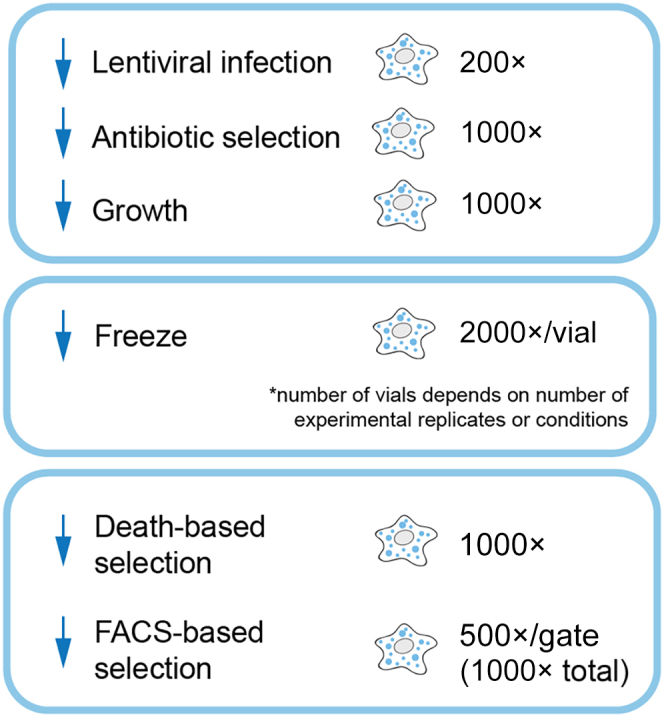
Schematic illustrating coverage maintenance at major steps of pooled CRISPR screens

Antibiotic selection

Timing: 1 week (FACS-based), 2–3 weeks (death-based)

• 12.Thaw cells in excess (2000× coverage) to prevent loss of coverage if cells die during thawing. Passage after 48 h and grow for another 48 h (96 h total).

CRITICAL: The number of passages and duration of growth can affect cellular phenotypes due to genetic compensation. When performing replicates or using multiple libraries in the same experiment, cells should be grown for the same number of days/passages.

The parameters of these steps will differ depending on whether the phenotypic selection is fluorescence-based or death-based.

• 13.
  Fluorescence-based screen.

  • a.
    Treat cells (if applicable).
  • b.
    Trypsinize (if using adherent cells) and collect cells in excess of 1000× coverage in FACS sorting media.

    Note: We recommend trypsinizing cells at >3000× coverage before FACS sorting to maintain a buffer in case of technical error and to account for sorting out any non-fluorescent cells. The number of cells that will be collected from cell sorting will be 1000× (500× in each gate). Sort cells and collect high and low fluorescence bins.

    Note: The FACS buffer used will depend on the characteristics of the cell line to be sorted. We use phenol red-free DMEM containing 3% FBS and 1% BSA for HuH7 cells.

    Note: The size of high-reporter and low-reporter bins affects the quality of screen data. A study⁵ computationally determined that collecting the highest 25% and lowest 25% bins results in the greatest signal-to-noise ratio. However, bin sizes can be altered depending on the biological question.¹¹ We have collected the top and bottom 30% fluorescence bins³ and recommend these parameters for FACS-based screens.

  • c.
    After sorting, spin cells at 500 × g for 10 min. Carefully aspirate FACS buffer and wash once with PBS. Spin cells again at 500 × g, remove PBS, and store cell pellets at −80°C.

• 14.
  Death-based screen.

  • a.
    Trypsinize and collect cells in media containing 10% FBS.
  • b.
    Count cells and seed in 245 mm square TC-treated culture dishes at 10% confluence (8–15 × 10⁶ cells, depending on the cell size).

    Note: The total amount of cells seeded should be above 1000× coverage. Use a minimum of 60 mL cell culture media containing the drug or vehicle at the desired concentration (determined in before you begin) for each plate.

  • c.
    Replace the media and drug/vehicle every 3 days and continue culturing the cells until they are confluent.
  • d.
    Repeat steps 14b–c until vehicle control treated cells divide >10 times (doubling cycles).
  • e.
    When cells reach >10 doubling cycles, harvest cells by trypsinization and wash once in media containing 10% FBS and once with PBS.
  • f.
    Spin cells at 500 × g for 5 min, aspirate PBS, and store cell pellet at −80°C. Each cell pellet should contain cells at >1000× coverage.

Preparing for deep sequencing

Timing: 1 week

To identify the sgRNAs present in each cell population, genomic DNA (gDNA) is extracted from frozen cell pellets and guide sequences are amplified by PCR.

CRITICAL: Cross contamination of libraries poses a huge risk to the integrity of screen results. To avoid contamination, some labs have designated spaces and hoods for these steps. At the very least, it is essential to thoroughly clean workspaces and equipment (e.g., pipettes, tube racks) with RNase Away (Thermo # 7002PK) or ELIMINase (Decon Labs # 1101) before the experiment and routinely wipe the bench surface and all pipettes during sample processing. Filtered pipette tips are essential. We recommend having a set of designated equipment for DNA processing.

• 15.Extract gDNA from cell pellets using Qiagen QIAamp DNA Blood Midi Kit (Cat # 51183) according to manufacturer’s instructions (link).

Note: We slightly modified this protocol for increased yield. For the DNA precipitation step, increase the spin time if centrifuging at a slower speed to fully precipitate DNA. Elute with Qiagen Buffer EB (10 mM Tris-Cl, pH 8.5; Cat # 19086) instead of Buffer AE. Spin at 4,500 × g for 5 min. Elute 2–3 times with new Buffer EB each time (do not reload eluate).

• 16.Measure the gDNA concentration by nanodrop. We typically obtain 100 μg gDNA per 20 × 10⁶ cells.

Note: Although measuring DNA by Qubit dsDNA assay is more sensitive and accurate than by nanodrop, we noticed running PCRs based on the concentration of gDNA from the Qubit assay sometimes resulted in a poor amplifying efficiency. Therefore, we recommend using a nanodrop to measure DNA concentration.

• 17.Amplify the integrated sgRNA (PCR1) with the following reagents and reaction program:

CRITICAL: To make sure the diversity and coverage of sgRNAs is not lost during PCR1, multiple 100 μL PCR reactions are required for screen preparation. Empirically, we recommend 1 PCR reaction for every 2,500 sgRNA in the library (e.g., For a customized library that has 25,000 sgRNAs, at least 10 PCR reactions are needed, and therefore a minimum of 100 μg gDNA is required).

Note: Although this protocol calls for 10 μg of genomic DNA per 100 μL PCR1 reaction, DNA input can be decreased to 5 μg or less if necessary. See troubleshooting section for a brief explanation on why a user may want to decrease the amount of input genomic DNA.

PCR1 reaction master mix

Reagent	Volume (μL)
gDNA template (10 μg)	x
Herculase II polymerase	2
oMCB_1562 (100 μM)	1
oMCB_1563 (100 μM)	1
5× Herculase buffer	20
dNTPs (100 nM)∗	1
ddH2O	75-x

∗25 nM per dNTP.

PCR1 cycling conditions

Steps	Temperature	Time	Cycles
Initial Denaturation	98°C	2 min	1
Denaturation	98°C	30 s	18 cycles
Annealing	59.1°C	30 s
Extension	72°C	45 s
Final extension	72°C	3 min	1
Hold	4°C	∞

Note: As the amount of genomic DNA collected from cell samples can be limited, especially for FACS-based screens, it is highly recommended to run a single (or “pilot”) PCR1 to ensure all conditions are correct and yield an amplified fragment.

• 18.Pool and mix all amplicons of the PCRs from the same gDNA sample. Add Illumina sequencing indexes with the following reagents and reaction program:

PCR2 reaction master mix

Reagent	Amount (μL)
PCR1 product	5
Herculase II polymerase	2
oMCB_1440 (100 μM)	0.8
oMCB_1439 (100 μM)	0.8
5× Herculase buffer	20
dNTPs (100 nM)	2
ddH2O	69.4

PCR2 cycling conditions

Steps	Temperature	Time	Cycles
Initial Denaturation	98°C	2 min	1
Denaturation	98°C	30 s	20 cycles
Annealing	59.1°C	30 s
Extension	72°C	45 s
Final extension	72°C	3 min	1
Hold	4°C	∞

Note: Though PCR1 uses 18 cycles, it was empirically determined that 20 cycles for PCR2 resulted in the best signal-to-noise ratio.

Note: Selecting index adapters with diverse sequences for pooled libraries is CRITICAL: for successful sequencing and data analysis. For information on how to optimize the color balance of the index adapters see the “Index Adapters Pooling Guide” published by Illumina (link).

Note: Only one 100 μL PCR2 reaction is sufficient to achieve sequencing depth.

• 19.Load PCR products onto 2% TBE-agarose gel.
• 20.Run the sample at 120 V for 50 min. Excise the brightest band.

Note: The size of the band is expected to be 280 bp but may run higher due to overloading of the gel.

• 21.Purify DNA products using QiaQuick Gel Extraction Kit (Cat # 28706) according to manufacturer’s instructions (link).

Note: We slightly modified this protocol for increased yield. When dissolving the gel, add 4 volumes Buffer QG instead of 3. For the DNA precipitation step, add 3 M sodium acetate pH 5.2 at a 1:100 ratio. For the wash step, wash with Buffer PE two times instead of once. Elute DNA in Buffer EB, not water.

• 22.Check DNA concentration by Qubit dsDNA HS Assay. We typically obtain 30 ng/mL DNA.
• 23.Verify DNA quality using a fragment analyzer. DNA fragments should run as a single band at ∼300 bp (Figure 6B).

• 24.
  If the DNA runs as a single band at ∼300 bp without contamination at other sizes, pool equal amounts of DNA from each screen sample so that the final concentration is 3 nM. Send the pooled library for deep sequencing.

  Note: The molecular weight of the DNA can be calculated based on the nucleotide sequence.

  • a.
    We typically send 50 μL of the pooled library at 3 nM and 30 μL of the Bassik custom sequencing Illumina sequencing primer (oMCB1672_new10gCRKO) at 100 μM. Both are sent in Qiagen EB (10 mM Tris, pH 8.5).

    CRITICAL: The pooled library loses diversity after ∼26 bp. For the sequencing read, 22–25 cycles single end read is recommended. Alternatively, request the sequencing facility to add 20%–30% PhiX to increase the diversity.

    Note: A minimum of 200× coverage is required when choosing a sequencing platform. For example, if a sgRNA library contains 30,000 elements, a pooled DNA library from 2 cell samples and 20% PhiX requires 30,000 × 200 × 2 × (100% + 20%) = 14.4 × 10⁶ single-end read. A standard MiSeq v3 has up to 25 × 10⁶ reads, which is enough to sequence this library.

    Note: We recommend requesting the sequencing data in the demultiplexed FASTQ format, as demultiplexing separates each barcoded sample reads into individual files.

Figure 6.

Troubleshooting DNA sequencing and analysis

(A) Example 2% agarose-TBE gel with a control lane (no gDNA control) and 7 samples (lanes A-G) following PCR2. Samples A and B were amplified as expected, with strong PCR2 amplicon bands at ∼300 bp. Amplification of samples C–G was inefficient, as indicated by a weaker PCR2 band (sample G) or no PCR2 band (sample C-F; red arrows).

(B) Example DNA quality control of a single sample by fragment analyzer. The DNA sample is highlighted in red with a strong peak ∼300 bp. Upper control marker (UM) and lower control marker (LM) bands are also highlighted.

(C–E) Negative control sgRNA cloud plots generated by the plotGenes script. The same library was sorted at 200× (C), 500× (D), and 1000× (E) coverage. As sgRNA representation increases, the distribution of negative control sgRNAs becomes tighter.

Analysis of deep sequencing data using casTLE

Timing: 2–5 days, not including any additional time needed by the facility performing the sequencing

Analysis of deep sequencing reads can be performed using a number of statistical frameworks, all of which involve sequence read alignment and gene enrichment calculations to identify hit genes that influence the phenotype of interest. Commonly used pipelines include MAGeCK,^12,13 MAGeCK-iNC,¹⁴ HiTSelect,¹⁵ DeSEQ,¹⁶ and RIGER.¹⁷ Here we describe the analysis pipeline for cas9 high-Throughput maximum Likelihood Estimator (casTLE⁸). The casTLE package consists of custom scripts for sequence read alignment using Bowtie, hit gene identification, and quality control and data visualization. CasTLE is built upon an empirical Bayseian framework that combines measurements from multiple targeting reagents (e.g., multiple sgRNAs per gene) to estimate a maximum effect (phenotype) size and an associated p-value by comparing each set of gene-targeting guides to the negative controls. For each gene, casTLE calculates enrichment (casTLE effect) as a median normalized log ratio of counts, with an associated confidence score (casTLE score), which is twice the log-likelihood ratio of the effect. CasTLE can analyze two replicate screens side-by-side, and a combination gene score and effect can then be calculated for each gene. CasTLE also contains plotting scripts, which allow the user to visualize the results as a volcano plot (see step 31), plot the distribution of targeting guides relative to negative controls (see step 36), graph and calculate guide representation (see step 30), and assess reproducibility between samples (see step 35).

• 25.Download and back up raw sequencing FASTQ files.

Note: Many NGS core facilities delete the FASTQ files after a few weeks, so download and back them up shortly after receiving them.

Note: Raw FASTQ files must be unzipped to be opened in a text editor. It is usually unnecessary to view them unless a potential quality issue is detected as the files are large and time consuming to download.

Note: FASTQC (link) can be used for a quality control assessment of FASTQ files (e.g., identification of irregularities, such as overrepresented sequences).

• 26.Install casTLE version 1.0 (link) and the required modules (link). We recommend running casTLE on Linux or MacOS.

Note: CasTLE scripts were written for python 2.7 (link) and Bowtie version 1 (link).

Note: Install the parallel python module (link) to increase speed of the casTLE analysis (optional but recommended).

Note: Alternatively, casTLE analysis workflow can be run on the new, web-based platform LatchBio (https://latch.bio/).

• 27.Open Terminal and navigate to the folder containing the casTLE scripts. CasTLE scripts are run from the command line.

Note: All casTLE scripts should be run from the top folder.

• 28.For screens conducted using sgRNA libraries other than the Bassik Human or Mouse CRISPR Knockout Library (Addgene # 101926-34, # 1000000121-30), create a bowtie index using the casTLE script makeIndices.py.

Note: If using the Bassik Human or Mouse CRISPR Knockout Library, skip this step and proceed to step 29.

python Scripts/makeIndices.py <list sequence file> <screen type> <screen type index>

List sequence file	The comma-delimited reference library file containing two columns: Element name, element sequence
Screen type	User-chosen name for the screen type (will need this name for the alignment script in step 29)
Screen type index	User-chosen name for the output bowtie index files (.ebwt) in the “Indices” folder

Note: In the event of the error bowtie-build: not found rerun the script with -b <bowtie-build location> at the end of the command. The error indicates that bowtie-build (the bowtie script required for casTLE’s makeIndices.py script) cannot be located, and -b will indicate the location.

• 29.Align FASTQ sequences to the reference sgRNA library using the casTLE script makeCounts.py.

python Scripts/makeCounts.py <file base for FASTQ file> <output file name> <screen type>

File base for FASTQ file	Path to the raw FASTQ file (can be .fastq or the zipped fastq.gz)
Output file name	User-chosen name of the output count file and corresponding record file
Screen type	The name of the screen type. If using Bassik libraries, the screen type is Cas9-10 (human) or mm-Cas9-10 (mouse). If using a different library, the screen type was named in step 28.

Note: To change the length of the sequencing read to be aligned, include the conditional argument -r [number] in which the number indicates how many base pairs should be used in the alignment. CasTLE’s default read length is 17 base pairs.

Note: If using a library other than the Bassik human or mouse library, the naming scheme for control sgRNAs (as used in the list sequence file) must be indicated. At the end of the argument, include -n [prefix of negative control sgRNAs].

• 30.Visualize the distribution of elements in each count file using the casTLE script plotDist.py (Figure 5A). The output is a .png file containing a plot of elements (x-axis) versus frequency (y-axis).

python Scripts/plotDist.py <output file name> <count file >

Output file name	User-chosen name of the output file
Count file	Path to the .csv count file generated in step 29

Figure 5.

CasTLE analysis of deep sequencing data

(A) Example output from the casTLE plotDist.py script. Counts for each element were normalized to the total number of counts and diversity was calculated as normalized entropy using the total number of elements to define the max entropy.

(B) Example volcano plot of casTLE effects versus casTLE scores calculated using the casTLE analyzeCounts.py script. The plot was created in GraphPad Prism.

(C and D) Reproducibility plots of casTLE scores (C) and casTLE effects (D) generated using the casTLE plotRep.py script.

(E–G) Example cloud plots and histograms for a hypothetical CRISPR screen showing genes with multiple enriched sgRNAs (E), multiple disenriched sgRNAs (F), or sgRNAs that were neither enriched nor disenriched (G). Cloud plots (top panels) show individual element counts of negative sgRNAs (grey) and sgRNAs targeting the gene of interest (color). Histograms (bottom panels) plot the null distribution (negative sgRNAs; red) and the distribution of sgRNAs targeting the gene of interest (blue), with each solid vertical line indicating the casTLE effect of an individual sgRNA and the dashed vertical line denoting that gene’s casTLE effect.

To visualize element distributions from more than one count file (e.g., three counts files), run the following script:

python Scripts/plotDist.py <output name> <count file 1> <count file 2> <count file 3> -l Sample1 Sample2 Sample3

Where -l indicates sample names to be included in the plot’s legend, in order of count files in the command.

Note: If analyzing counts from a specific sublibrary within the Bassik library, indicate the sublibrary with -x [sublibrary]. For example, -x ACOC.

• 31.Compare sgRNA enrichment between two files (e.g., vehicle vs. treated or GFP high vs. GFP low) using the casTLE script analyzeCounts.py.

python Scripts/analyzeCounts.py <count file 1> <count file 2> <output results file>

Count file 1	Path to the counts file for sample 1 (e.g., untreated or vehicle treated for death-based screen, low fluorescence population for FACS-based screen)
Count file 2	Path to the counts file for sample 2 (e.g., drug treated for death-based screen, high fluorescence population for FACS-based screen)
Output results file	User-chosen name of the output results file and corresponding record file

The output is a .csv file (and an associated record file) containing 13 columns:

Column	Heading	Description
A	GeneID	Ensembl ID
B	Gene symbol	Gene name
C	GeneInfo	Identifier
D	Localization	GO term
E	Process	GO term
F	Function	GO term
G	Element #	Number of sgRNAs targeting that gene detected
H	casTLE effect	Most likely effect size
I	casTLE score	Confidence in the casTLE effect
J	casTLE p-value	Estimated p-value from the casTLE score. This column will read N/A until the addPermutations.py script is run (step 32)
K	Minimum effect estimate	95% credible interval for the casTLE effect size estimate
L	Maximum effect estimate	95% credible interval for the casTLE effect size estimate
M	Individual elements	Individual element (sgRNA) enrichments. Formatted as <enrichment value> : <element ID>

Note: By default, casTLE removes sgRNAs with fewer than 10 sgRNA counts from the analysis. To change the threshold for removal, include -t [number] at the end of the argument. For example, -t 50 will tell casTLE to remove genes with fewer than 50 counts from the analysis.

Note: The casTLE script plotVolcano.py can be used to quickly visualize the casTLE effect (x-axis) versus casTLE score (y-axis). We recommend generating volcano plots in a program such as GraphPad Prism for publication quality figures (Figure 5B).

• 32.
  Estimate p-values using the casTLE script addPerm.py and calculate false discovery rate (FDR).

  python Scripts/addPermutations.py <results file> <number of permutations>

  Results file	Path to the results file generated in step 31
  Number of permutations	User-chosen number of permutations

  Note: For publication, we recommend that the number of permutations run is 50× the number of genes in the library. For example, run 150,000 permutations for a library that contains 3,000 genes.

  • a.
    To calculate 10% FDR, sort genes from lowest to highest p-value and use the following equation: =IF([p-value]<0.1×(ROW()-1)/[total # of genes],1,[subsequent row]).

• 33.Compare screens using the casTLE script analyzeCombo.py. The output file will contain a new, combined casTLE effect and casTLE score for each gene.

python Scripts/analyzeCombo.py <results file 1> <results file 2> <output file name>

Results file 1	Path to the results file for replicate 1
Results file 2	Path to the results file for replicate 2
Output file name	User-chosen name of the output results file and corresponding record file

• 34.Estimate p-values for the combined casTLE results using the casTLE script addCombo.py. Calculate false discovery rate (FDR) as described in step 32.

• python Scripts/addCombo.py <combo results file> <number of permutations>

• 35.Compare casTLE effects and casTLE scores between replicates using the casTLE script plotRep.py (Figures 5C and 5D). The output is two scatter plots (PNG files) with the coefficient of determination (R²).

python Scripts/plotRep.py <results file 1> <results file 2> <output file name>

• 36.Visualize distribution of sgRNAs for genes of interest versus null distribution using the casTLE script plotGenes.py (Figures 5E–5G).

python Scripts/plotGenes.py <results file 1> <gene name 1> <gene name 2>…

Note: The output is a cloud plot and a histogram. The cloud plot (top panels) is a scatter plot showing the deep sequencing counts for each element targeting the gene of interest (color scale) along with all the negative sgRNAs (gray). The histogram (bottom panels) is a frequency distribution of the casTLE effect for negative controls (red) versus the gene of interest (blue). Vertical solid lines indicate the individual casTLE effects for each guide, and the vertical dashed line indicates the casTLE effect for that gene. Figures 5E–5G shows examples of cloud plots and histograms for hypothetical enriched gene X (Figure 5E), depleted gene Y (Figure 5F), and unaffected gene Z (Figure 5G).

Note: This script also serves as a quality control step by plotting the distribution of negative control sgRNAs, in both the cloud plot and the histogram.

Note: To change the file type, add -f [file type] to the end of the command. For example, to generate SVG files instead of PNG files, the script should end with -f svg, and the output file will be a SVG file.

Expected outcomes

If the PCR is successful, a clean, bright band at ∼300 bp from PCR2 product should be visible on the 2% TBE-agarose gel. If amplicons from PCR1 are also loaded onto the agarose gel, it is not uncommon if only a very faint band or no band is seen.

For the fragment analysis, 3 peaks are expected, including a lower marker (LM) at 1 bp, an upper marker (UM) at 6,000 bp and a single peak at ∼300 bp from the DNA sample (Figure 6B).

For successful sequencing, several files in “fastq.gz” and “fastq.gz.md5” format should be generated. The “fastq.gz.md5” file contains a string of numbers and letters called md5 hash, which are identifiers of the corresponding “fastq.gz” file. It is important to check the md5 hash of each “fastq.gz” file and ensure they are identical to the record in “fastq.gz.md5” files. For a single-read run, one R1 fastq file will be created for each sample. In addition to all files associated with each sample, files named as “undetermined” could also be included. They contain sequences that have not been successfully demultiplexed on the barcode with sufficient accuracy. If PhiX is spiked in, they should also be in the “undetermined” files. Only “fastq.gz” files with the sample name are needed for the analysis.

A successful CRISPR screen should maintain high sgRNA diversity (>0.9), calculated in step 35. If diversity is lower, proceed to the troubleshooting section. CasTLE effects are standardly between 0 and 8 and casTLE scores between 0 and 500. A false discovery rate (FDR) based on casTLE effect or score can be calculated to determine “hit” genes (see step 32). The FDR cutoff will depend on the biological question, whether identifying larger compendiums of moderate- to high-confidence hits or a select few of the highest confidence hits. We use a 10% FDR for the former and a 1% or 5% FDR for the latter.

After identifying hit genes, single gene KOs should be generated to validate effects seen in the CRISPR screen. At least two independent sgRNAs should be used to mitigate false positives. The most effective sgRNAs to use for follow-up studies can be identified from the results files and counts file as well as the cloud and histogram plots made by the plotGenes script (see step 36). In a successful CRISPR screen, single KOs should replicate the effects determined by bioinformatic analysis (see troubleshooting for an explanation on why strong, real hits may not validate as individual KOs).

To further compare results and determine biological significance, data should be uploaded onto a CRISPR screen repository such as BioGRID CRISPR repository, CRISPRbrain, or CRISPRlipid.

Limitations

Compared to arrayed CRISPR/Cas9 screens, which analyze genetic perturbations independently and can therefore be paired with imaging or metabolomics profiling,¹⁸ pooled screens give limited insight into how individual perturbations affect cellular phenotypes besides the one in question. The generation of individual gene knockouts is necessary to validate and expand upon screen results. Although pooled screens are less labor-intensive than arrayed screens, they still require at least one month of cell culture, which incurs a high cost, made higher by using adherent cells and growing them at high coverage. Depending on the question of interest, using suspension cells can lower the time and cost of a genetic screen. And, although proficiency in Python is not necessary for running casTLE commands, a basic understanding of coding is useful for performing bioinformatic analysis. Analytical platforms like LatchBio negate the need for coding experience and make analysis more accessible to researchers of different backgrounds.

False positive and false negative “hits” are possible and must be mitigated at every step of the screening process. False positives can occur when sgRNAs bind off-target sites or gene expansion causes Cas9 to cleave many times, leading to upregulation of the DNA damage response.¹⁹ False negatives can occur when coverage is low or lost (Figures 6C–6E), or compensation occurs genetically or arises during the screening process.^20,21 It is therefore necessary to maintain cells at high (1000×) coverage and to grow and passage cell samples for the same length of time to prevent genetic compensation. Performing multiple replicates and using the combination analysis function of casTLE also addresses the problem of false negatives.⁸

Troubleshooting

Problem

Low titer of lentivirus packaged sgRNA library.

Potential solution

• •Poor DNA quality: Check that the pooled library is pure (260/280 and 260/230 values).
• •Issues with HEK293T cells: Cells should be low passage and seeded at the optimal confluence for transfection. Check the viability of HEK cells prior to seeding and aim for over 95% viability.
• •Issues with transfection reagents: Double-check that reagents are not expired and/or have precipitated.
• •Packaging vector issues: Ensure that the correct packaging vectors are being used (e.g., 2nd versus 3rd generation).
• •Filtering through wrong pore size: Virus-containing media should be filtered through a 0.45 μm mesh, not 0.20 μm.
• •Insufficient viral production: include a positive control, such as plasmid that has been packaged successfully in the lab.
• •If viral titer is still low, concentrate virus using a reagent such as PEG-it Virus Precipitation Solution (System Biosciences # LV810A-1).

Problem

Inefficient PCR or no PCR product (Figure 6A).

Potential solution

• •Ethanol carryover from the genomic DNA extraction can inhibit downstream PCR reactions. Prior to eluting gDNA, incubate columns at 70°C for 10 min to evaporate residual ethanol.
• •Decrease the gDNA input to ∼5 μg per PCR1 reaction (step 22). Use nanodrop concentrations of purified gDNA instead of Qubit concentrations.
• •If samples were successfully amplified but with low efficiency (Figure 6A, lane G), increase the number of PCR1 cycles to 19–20 cycles.

Problem

Low percentage of successfully mapped reads.

Potential solution

Open the FASTQ from the NGS facility in a text editor and look at the sequences to better understand the problem. NGS sequences may need to be trimmed during the read mapping step (casTLE makeCounts.py command).

Problem

Low library diversity or loss of element representation.

Potential solution

Low library diversity often results from (1) problems with the sgRNA library, (2) bottlenecks during the screening process, or (3) issues with deep sequencing preparation.

• •The sgRNA library should always be sequenced before the first use to ensure that roughly 90% of guides are present and evenly distributed. If the library is missing more than 10% of elements, it should be re-amplified.
• •
  Bottlenecks can occur during lentiviral packaging of sgRNA library, infection, and passaging.

  • ○
    Ensure that library representation will be maintained by transfecting the necessary number of HEK293T cells with enough library DNA.
  • ○
    Perform quality control (see steps 27 and 28) on NGS sequences from the initially library-infected cell population to determine whether the bottleneck occurred prior to phenotypic selection.
  • ○
    Cells should always be passaged at ≥ 1000× coverage.
• •A common limiting step in deep sequencing preparation is the gDNA extraction. When planning the screen, the user should ensure that enough cells can be collected to harvest a sufficient amount of gDNA. We typically collect 1000× cells (1000× number of gRNAs). For example, in a FACS-based screen of a 30,000 sgRNA library, at least 30 × 10⁶ cells should be collected (total).

Problem

Hit genes determined by casTLE are not replicating effects in individual knockout cell lines.

Potential solution

Some strong hits are difficult to validate as single knockouts, due to cell non-autonomous effects, viability issues when cultured with other non-KOs, or other influences on the phenotype due to culture conditions that make it difficult to compare to non-targeting controls in separate wells.

• •Prior to generating individual knockout cell lines, perform a secondary pooled screen (also known as a batch retest screen) of a custom sgRNA library consisting of significant hit genes and control sgRNAs.
• •Culture individual KO cell lines together with non-targeting cells, using different fluorescent markers.

Resource availability

Lead contact

Further information and requests for resources and reagents should be directed to the corresponding authors, Zhipeng Li (li.zhipeng@berkeley.edu) or James A. Olzmann (olzmann@berkeley.edu).

Materials availability

This study did not generate new unique reagents.

Data and code availability

This study did not generate any codes. All experimental data in the paper are available upon reasonable request to the lead contact.

References

- 1.Bersuker K., Hendricks J.M., Li Z., Magtanong L., Ford B., Tang P.H., Roberts M.A., Tong B., Maimone T.J., Zoncu R., et al. The CoQ oxidoreductase FSP1 acts parallel to GPX4 to inhibit ferroptosis. Nature. 2019;575:688–692. doi: 10.1038/s41586-019-1705-2. [DOI] [PMC free article] [PubMed] [Google Scholar]
- 2.Li Z., Ferguson L., Deol K.K., Roberts M.A., Magtanong L., Hendricks J.M., Mousa G.A., Kilinc S., Schaefer K., Wells J.A., et al. Ribosome stalling during selenoprotein translation exposes a ferroptosis vulnerability. Nat. Chem. Biol. 2022;18:751–761. doi: 10.1038/s41589-022-01033-3. [DOI] [PMC free article] [PubMed] [Google Scholar]
- 3.Roberts M.A., Deol K.K., Lange M., Leto D.E., Mathiowetz A.J., Stevenson J., Hashemi S.H., Morgens D.W., Easter E., Heydari K., et al. Parallel CRISPR-Cas9 screens reveal mechanisms of PLIN2 and lipid droplet regulation. Cell Biol. 2022 doi: 10.1101/2022.08.27.505556. [DOI] [PMC free article] [PubMed] [Google Scholar]
- 4.Hayashi H., Kubo Y., Izumida M., Matsuyama T. Efficient viral delivery of Cas9 into human safe harbor. Sci. Rep. 2020;10 doi: 10.1038/s41598-020-78450-8. [DOI] [PMC free article] [PubMed] [Google Scholar]
- 5.Nagy T., Kampmann M. CRISPulator: a discrete simulation tool for pooled genetic screens. BMC Bioinf. 2017;18:347. doi: 10.1186/s12859-017-1759-9. [DOI] [PMC free article] [PubMed] [Google Scholar]
- 6.Iyer V.S., Jiang L., Shen Y., Boddul S.V., Panda S.K., Kasza Z., Schmierer B., Wermeling F. Designing custom CRISPR libraries for hypothesis-driven drug target discovery. Comput. Struct. Biotechnol. J. 2020;18:2237–2246. doi: 10.1016/j.csbj.2020.08.009. [DOI] [PMC free article] [PubMed] [Google Scholar]
- 7.Morgens D.W., Wainberg M., Boyle E.A., Ursu O., Araya C.L., Tsui C.K., Haney M.S., Hess G.T., Han K., Jeng E.E., et al. Genome-scale measurement of off-target activity using Cas9 toxicity in high-throughput screens. Nat. Commun. 2017;8 doi: 10.1038/ncomms15178. [DOI] [PMC free article] [PubMed] [Google Scholar]
- 8.Morgens D.W., Deans R.M., Li A., Bassik M.C. Systematic comparison of CRISPR/Cas9 and RNAi screens for essential genes. Nat. Biotechnol. 2016;34:634–636. doi: 10.1038/nbt.3567. [DOI] [PMC free article] [PubMed] [Google Scholar]
- 9.Langmead B., Trapnell C., Pop M., Salzberg S.L. Ultrafast and memory-efficient alignment of short DNA sequences to the human genome. Genome Biol. 2009;10:R25. doi: 10.1186/gb-2009-10-3-r25. [DOI] [PMC free article] [PubMed] [Google Scholar]
- 10.Langmead B., Salzberg S.L. Fast gapped-read alignment with Bowtie 2. Nat. Methods. 2012;9:357–359. doi: 10.1038/nmeth.1923. [DOI] [PMC free article] [PubMed] [Google Scholar]
- 11.Leto D.E., Morgens D.W., Zhang L., Walczak C.P., Elias J.E., Bassik M.C., Kopito R.R. Genome-wide CRISPR analysis identifies substrate-specific conjugation modules in ER-associated degradation. Mol. Cell. 2019;73:377–389.e11. doi: 10.1016/j.molcel.2018.11.015. [DOI] [PMC free article] [PubMed] [Google Scholar]
- 12.Li W., Xu H., Xiao T., Cong L., Love M.I., Zhang F., Irizarry R.A., Liu J.S., Brown M., Liu X.S. MAGeCK enables robust identification of essential genes from genome-scale CRISPR/Cas9 knockout screens. Genome Biol. 2014;15:554. doi: 10.1186/s13059-014-0554-4. [DOI] [PMC free article] [PubMed] [Google Scholar]
- 13.Wang B., Wang M., Zhang W., Xiao T., Chen C.-H., Wu A., Wu F., Traugh N., Wang X., Li Z., et al. Integrative analysis of pooled CRISPR genetic screens using MAGeCKFlute. Nat. Protoc. 2019;14:756–780. doi: 10.1038/s41596-018-0113-7. [DOI] [PMC free article] [PubMed] [Google Scholar]
- 14.Tian R., Abarientos A., Hong J., Hashemi S.H., Yan R., Dräger N., Leng K., Nalls M.A., Singleton A.B., Xu K., et al. Genome-wide CRISPRi/a screens in human neurons link lysosomal failure to ferroptosis. Nat. Neurosci. 2021;24:1020–1034. doi: 10.1038/s41593-021-00862-0. [DOI] [PMC free article] [PubMed] [Google Scholar]
- 15.Diaz A.A., Qin H., Ramalho-Santos M., Song J.S. HiTSelect: a comprehensive tool for high-complexity-pooled screen analysis. Nucleic Acids Res. 2015;43:e16. doi: 10.1093/nar/gku1197. [DOI] [PMC free article] [PubMed] [Google Scholar]
- 16.Anders S., Huber W. Differential expression analysis for sequence count data. Genome Biol. 2010;11:R106. doi: 10.1186/gb-2010-11-10-r106. [DOI] [PMC free article] [PubMed] [Google Scholar]
- 17.Luo B., Cheung H.W., Subramanian A., Sharifnia T., Okamoto M., Yang X., Hinkle G., Boehm J.S., Beroukhim R., Weir B.A., et al. Highly parallel identification of essential genes in cancer cells. Proc. Natl. Acad. Sci. USA. 2008;105:20380–20385. doi: 10.1073/pnas.0810485105. [DOI] [PMC free article] [PubMed] [Google Scholar]
- 18.Bock C., Datlinger P., Chardon F., Coelho M.A., Dong M.B., Lawson K.A., Lu T., Maroc L., Norman T.M., Song B., et al. High-content CRISPR screening. Nat. Rev. Methods Primers. 2022;2:8. doi: 10.1038/s43586-021-00093-4. [DOI] [PMC free article] [PubMed] [Google Scholar]
- 19.Sheel A., Xue W. Genomic amplifications cause false positives in CRISPR screens. Cancer Discov. 2016;6:824–826. doi: 10.1158/2159-8290.CD-16-0665. [DOI] [PMC free article] [PubMed] [Google Scholar]
- 20.Krshnan L., Siu W.S., Van de Weijer M., Hayward D., Guerrero E.N., Gruneberg U., Carvalho P. Regulated degradation of the inner nuclear membrane protein SUN2 maintains nuclear envelope architecture and function. Elife. 2022;11 doi: 10.7554/eLife.81573. [DOI] [PMC free article] [PubMed] [Google Scholar]
- 21.Rossi A., Kontarakis Z., Gerri C., Nolte H., Hölper S., Krüger M., Stainier D.Y.R. Genetic compensation induced by deleterious mutations but not gene knockdowns. Nature. 2015;524:230–233. doi: 10.1038/nature14580. [DOI] [PubMed] [Google Scholar]
Associated Data
This section collects any data citations, data availability statements, or supplementary materials included in this article.
Data Availability Statement