Box dimension of the border of Kingdom of Saudi Arabia

Abstract

Fractal dimension unlike topological dimension is (usually) a non-integer number which measures complexity, roughness, or irregularity of an object with respect to the space in which the set lies. It is used to characterize highly irregular objects in nature containing statistical self-similarity such as mountains, snowflakes, clouds, coastlines, borders etc.

In this article, box dimension (a version of fractal dimension) of the border of Kingdom of Saudi Arabia (KSA) is computed using a multicore parallel processing algorithm based on the classical box-counting method. A power law relation is obtained from numerical simulations which relates the length of the border with the scale size and provides a very close estimate of the actual length of the KSA border within the scaling regions and scaling effects on the length of KSA border are considered. The algorithm presented in the article is shown to be highly scalable and efficient and the speedup of the algorithm is computed using Amdahl's and Gustafson's laws. For simulations, a high performance parallel computer is employed using Python codes and QGIS software.

1. Introduction

Fractal geometry has evolved drastically over past few decades and researchers have described many natural, scientific and engineering phenomena in the framework of fractal geometry which was not possible to achieve with tools from the classical Euclidean geometry. Fractals are ubiquitously found in natural objects, for examples in trees, snowflakes, mountains, crystals etc. and are visually attractive to human eyes. Broadly speaking a fractal is an irregular geometric object that may repeat its geometry at smaller (or larger) scales called self-similarity and has a (non-integer) fractal dimension.

Since the pioneering works by Mandelbrot [1], [2], [3], [4], fractals have been studied in almost every field of science and engineering including mathematics, computer science, physics, chemistry, biology, geology, social science, economics, engineering, technology, art, architecture, etc. Fractals and their applications have high potential to expand further encompassing many interdisciplinary and evolving fields of research. Recent survey articles by Husain et al. [5], [6] presents an eclectic review of fractals along with mathematical description, aesthetic, artistic, and architectural engineering, industry, commercial, and futuristic applications of fractals ranging from aesthetic designs in art, fashion designing, landscape generation, tessellations, fractal image compression, fractal antennas, fracture mechanics and other evolving future ready applications.

Borders and coastlines have been of paramount interest for every country since they define geographical boundaries and provide means of transport for trade and other purposes between countries. The geometry of these naturally formed objects is random having fractal character (usually irregular, zigzag, and rugged having variations at multiple scales). In case of a smooth curve (for example, a circle) the length can be calculated using successive approximations by line segments and for much better results, smaller segments can be applied. However, borders and coastlines are not smooth therefore, their lengths can not be measured by this simple Euclidean geometry techniques due to inaccurate measurements and use of various approaches by different researchers leading to substantial differences in measuring the length. As a result, the methods based on Euclidean geometry are inadequate to characterize these objects accurately and it is desirable to find better means of describing the random geometries of borders and coastlines integrated with advanced computational methods and available software.

Fractal dimension of an object is as a quantification of roughness or irregularity present in an object. For any fractal, self-similar or not there are various versions of fractal dimension studied in the literature, for example, box-dimension, similarity dimension, divider dimension, Higuchi dimension, correlation dimension, Minkowski dimension, inductive dimension and so on. All of these provide a means to compare the size of fractals mathematically relative to the underlying space. For certain well behaved fractals (e.g., self-similar) these different dimensions are equal whereas for random and irregular geometries (e.g., coastlines, time-series data, turbulent flows etc.) they yield different values. All these dimensions can be regarded as variants of a more abstract dimension called Hausdorff dimension which is based on measures and the reader may refer to Barnsley [7], Falconer [8]), Frame et al. [9] and Edgar [10] for a collated work of different kinds of fractal dimensions as well as many interesting results connecting them together.

Many real world objects and entities in nature exhibit fractal properties and calculation of fractal dimension is a classical problem which has applications in diagnostic imaging (e.g., in characterizing cells and tissues, ophthalmology [11], [12]), neuroscience (e.g., in treatment of Alzheimer's and brain related diseases [13]), electrochemistry [14], image compression, telecommunications (e.g., fractal antennas), astronomy (e.g., in observing and analyzing turbulence in terrestrial bodies [15]), earth sciences (e.g., in predicting compressive strength of volcanic welded bimrocks [16]), physics (e.g., superconductivity [17], evaluating fractal dimension of profiles [18]), urban planning [19], [20], [21], [22], [23], [24], [25], [26], magnetohydrodynamics (MHD) [27], combustion theory [28], geography [29], [30], fractal thermoelasticity [31], fluid dynamics [32], [33], [34], nuclear reactors [35], biology [36], meteorology [37] etc.

Among all types of fractal dimensions, the box-counting dimension is one of the classical and simplest type of fractal dimension which is also given by a power law relation like any other fractal dimension. It is calculated using the box-counting method in which a grid of boxes is imposed on the object and the count of boxes cutting across the object is stored at every decreasing scale to capture finer and finer details present in the geometry. Due to its simplicity and employability on computers, the box counting method can be used for any object making the box dimension more popular as compared to other fractal dimensions. Moreover, for many self-similar fractals it coincides with the abstract Hausdorff dimension.

The pioneering study on fractal dimension of borders and coastlines was started by Mandelbrot [1] in his expository article. Mandelbrot [1], [2], [3] proved that the fractal dimension of any object remains constant, while its length changes with the change in measurement scale. Since then fractal dimension of a number of land frontiers has been computed by many researchers and we refer to Husain et al. [38] for a summary of available results on fractal dimension of coastlines and borders.

We refer to the papers [25], [39], [40], [41], [42], [43], [44], [45], [46], [47], [48] for applicability of fractal dimension in several existing and evolving research areas. We also cite the book by Fernández-Martínez et al. [49] which generalizes fractal dimension to more common context of fractal structures. Use of GIS software such as ArcGIS, QGIS etc. has proven to be very effective in calculating fractal dimensions in the context of coastlines and other geological features.

In this work, we compute the box dimension of the border of Kingdom of Saudi Arabia (KSA). For this purpose, we use the box-counting method and a neoteric parallel processing algorithm introduced by Husain et al. [38] to speedup simulations. We discover a power law relation from computational results which provides an estimate of the length of the KSA border and consider the effects of length scales on length of the KSA border. In order to show the effectiveness of the algorithm we compute speedup of the algorithm using Amdahl's and Gustafson's laws.

The Kingdom of Saudi Arabia is the largest country in the Arabian peninsula which is situated at the crossroads of Europe, Asia and Africa. As per the official records (available at https://www.stats.gov.sa/en/), the total length of the KSA border (i.e., land frontier and coastline) is about 6,751 km. Out of this the land frontier is 4,431 km which is shared with 7 countries and 2,320 km is the coastline. The KSA coastline is divided into two parts east and west. The western coast is surrounded by the Red Sea and the Gulf of Aqaba, while the eastern coast goes around the Arabian Gulf.

KSA has the largest natural-resource deposits of oil and gas in the middle east as well as it is the largest exporter of oil in the world through its land frontier and coastline boundaries. The application of fractal dimension in various process of oil and gas production is already established (see Suleymanov [50] and reference therein). This makes the study important and exciting.

2. Classical methods to compute fractal dimension

Fractal geometry can model broken, irregular and rough shapes (e.g. coastlines) and the fractal dimension is a measure of roughness and complexity of an object. For instance, an object having a higher fractal dimension is more complex as compared to an object with lower fractal dimension.

By a metric space $(X,d)$, we mean a non-empty set X together with a non-negative distance function d (for instance, the Euclidean distance on ${\mathbb{R}}^m,m\ge 1$) defined on $X\times X$ satisfying the usual properties of a metric (see Edgar [10]). Here, $X\times X$ denotes the usual Cartesian product of two sets. Let $\mathcal{H}(X)$ denote the set of all non-empty compact (closed and bounded) subsets of X.

Definition 2.1

Let $A\in \mathcal{H}(X)$ and $ϵ>0$ (a typical length scale) be given. Then A is said to have fractal dimension D if there exists a positive constant C such that

$$N_{ϵ}\left(A\right)\approx C{ϵ}^{-D}.$$ (1)

Here, $N_{ϵ}(A)$ is the least number of closed balls needed to cover A.

In equation (1), the number $N_{ϵ}(A)$ make sense since A is compact and it follows that

$$D=\underset{ϵ\to 0}{\lim }\frac{\log (N_{ϵ}(A))}{\log \left(\frac{1}{ϵ}\right)}$$ (2)

provided the limit exists. Barnsley [7] proved that $D(A)$ consists for any $A\in \mathcal{H}({\mathbb{R}}^m)$, where ${\mathbb{R}}^m$ denotes the Euclidean plane (xy-plane for $m=2$ and xyz-plane for $m=3$). In particular, the fractal dimension makes sense for borders, coastlines, rivers, mountains and other natural objects since they are compact subsets of ${\mathbb{R}}^m$ for $m=2,3$. Since the border or coastline of any country is a compact subset of ${\mathbb{R}}^2$, therefore, the fractal dimension of a border or coastline is a numerical value that describes geometric complexity and randomness present in the geometry having a value between 1 and 2. Various methods have been explained in the previous works to calculate the fractal dimension of borders and coastlines (see Husain et al. [38] for more details and Table 1 for partial summary of results).

Table 1.

Divider and box dimensions of some coastlines. “−−−”denotes no data available.

Coastline	Divider Dimension (D)	Box-dimension (Db)	Reference(s)
Great Britain	1.25	−−−	Mandelbrot [1]
Australia	1.13	−−−	Mandelbrot [1]
Coastline of South Africa	1.02	−−−	Mandelbrot [1]
China	1.195	−−−	Su et al. [52]
Continental coastline of China	1.2004	1.0929	Ma et al. [53]
Coastline of Australia	−−−	1.143	Husain et al. [38]

There is no universally accepted definition of a border or coastline yet. Every country has its own way of defining coastline. A most common definition of a coastline is that it defines the boundary between land and sea which means that means the 0m contour line is next to the coastline.

Another type of fractal dimension is the divider dimension (also known as compass) which is more appropriate for characterization of land frontiers and coastlines since it is defined for all curves. A divider of step length ϵ is chosen and let $N(ϵ)$ be the total number of steps taken to travel the entire curve. Then the length of the curve is simply $L(ϵ)=N(ϵ)\times ϵ$. As ϵ decreases, on the one hand the finer features of the curve are incorporated but on the other hand the total length of the curve increases. Richardson [51] was the first to observe this phenomenon in his work on coastlines using the divider method. He found the power law relation connecting length with the step size as

$$L(ϵ)=k\times {ϵ}^{\alpha },$$ (3)

where k and α are constants.

Mandelbrot [1], [4] proved that $\alpha =1-D$. This provides us,

$$\log L(ϵ)=\log k+(1-D)\log ϵ.$$

A plot of $\log (ϵ)$ vs. $\log L(ϵ)$ is termed as the Richardson plot (also known as $\log -\log$ plot) and number D in the slope of the line is called the divider dimension.

From equation (3) with $\alpha =1-D$, we can write $ϵ\times N(ϵ)=k\times {ϵ}^{1-D}$. This allows us to write

$$\log N(ϵ)=\log k-D\log ϵ.$$ (4)

Thus, plotting $\log N(ϵ)$ against $\log ϵ$, the slope of the resulting line is −D.

At a given step size the divider method may fail to provide a good measurement at multiple forward intersections (which often in borders and coastlines). Another difficulty is that at any scale size is possible that some part of the curve (with length smaller than the scale size) is leftover to be measured which may direct to significant errors.

To overcome these obstacles, the well known box-counting method may be used which give rise to the box-counting dimension or more commonly known as the box dimension. There are also various versions of box-counting dimension and for curves, it is also given by a power law relation just like the divider dimension. It is possible to find box dimension of almost every object, it is simple to implement on computers and therefore considered as one of the most practical fractal dimension. Moreover, for many self-similar fractals it coincides with the Hausdorff dimension.

In box-counting method, a grid or mesh of boxes having size $ϵ\times ϵ$ is imposed on the given curve. Then, the number of boxes $N(ϵ)$ intersecting the curve are counted which increases as ϵ decreases. A plot of $\log N(ϵ)$ vs. $\log ϵ$ has approximate slope as $-D_b$. The number $D_b$ is called the box-counting dimension. The scaling hypothesis says that $N(ϵ)$ is related to ϵ by,

$$N\left(ϵ\right)=k\cdot {(1/ϵ)}^{D_b}.$$

Thus, the value of $D_b$ can be calculated in two ways. For some objects, an explicit formula for $N(ϵ)$ can be found and in that case $D_b$ is computed by taking a limit of the appropriate expression (see Theorem 2.1 below). For physical fractals and random fractals (such as coastlines and borders), an exact formula for $N(ϵ)$ may not be available. In such cases, $D_b$ is computed by measuring the slope of the $\log (N(ϵ))$ versus $\log (ϵ)$ graph.

As a particular case of equation (2), we have the box-counting theorem (Barnsley [7]),

Theorem 2.1 The box counting theorem —

Let A be a closed and bounded subset of${\mathbb{R}}^2({\mathbb{R}}^3)$. Cover A by square boxes of side length$\frac{1}{2^n}$. Let$N_n(A)$be the number of boxes that intersect A. Then the box-counting dimension of A is given by

$$D_b(A)=\underset{n\to \infty }{\lim }\left\{\frac{\log (N_n(A))}{\log (2^n)}\right\}.$$

Some authors [40], [53] have discussed the scaling region of coastlines which provides a means to determine the accurate value of the scale size for exact measurement of the length and fractal dimension calculation (see Dimri [40]). Thus, a careful analysis of the measurement scale is important to ensure if it is within the scaling region for accurate results. We have identified scaling regions for the border of KSA using our numerical results and plots.

3. Materials and methods

Just like other geological features, borders and coastline exhibit statistical self-similarity over a range of scales. Fig. 1 shows the border of KSA (obtained using QGIS) marked with thick black color for clarity. Our simulations are based on the novel multicore parallel processing algorithm presented in [38] written in Python and integrated with the QGIS software. We first select a high spatial resolution map of the KSA border from the GADM [55] database as a single ‘multi-polygon’ (a single feature) with longitude-latitude coordinate system. We then use the Saudi Arabia National Spatial Reference System (SANSRS) to transform it to a planar coordinate system. In our simulations, we have included only the terrestrial borders of KSA (marked with dark black color in Fig. 1. We did not consider marine borders or national waters and we have excluded all the islands (irrespective of the size i.e., large or small) in this study and only the mainland of the KSA is considered. For KSA coastline simulations we have developed a new algorithm in another upcoming work. All the islands (excluded from the study) are removed from the map by dividing the entire map into a group of features using an ‘R’-program and selecting the largest feature which corresponds to the mainland.

Figure 1.

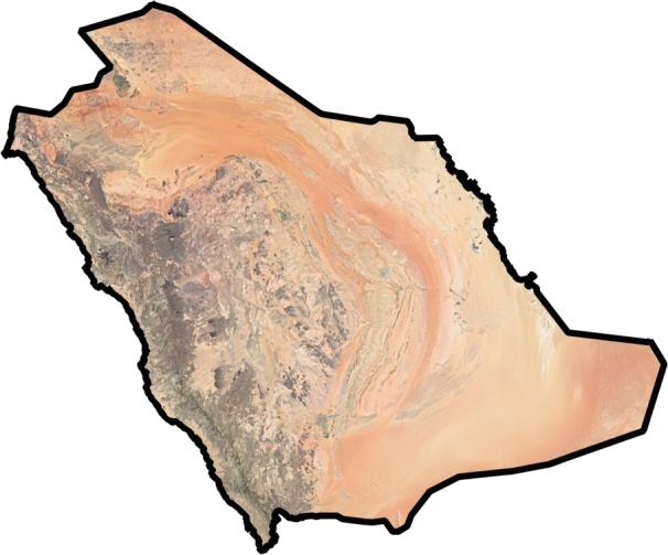
Border of the Kingdom of Saudi Arabia created using QGIS [54], Pi-version (available at https://qgis.org/downloads/).

A grid of square boxes of a chosen (input) size is superimposed on the mainland using grid layer tool in the QGIS and the number of boxes intersecting the border are counted. This process is iterated with different scales using a Python program. Flowchart of the process is given in Fig. 2.

Figure 2.

Flow chart of the method (Husain et al. [38]).

In the overall flow of our process in Fig. 2 after covering the border with grid layer tool in QGIS we apply the algorithm to obtain the count of boxes intersecting the border at various scales. On smaller scales, the number of boxes in the grid (superimposed on the curve) increases rapidly which makes the problem size very large and the box counting method becomes computationally slow. To speedup computations novel algorithms concerning parallel or multicore processing are needed. In parallel approach a group of boxes is mapped to a single processor on a machine with multiple processors and results from different processors are combined together to get the box count that intersect a given shape. A new multicore, embarrassingly parallel processing algorithm for computing box dimension was presented in [38] and successfully implemented to evaluate fractal dimension of the coastline of Australia. We compute the box dimension of KSA border using this algorithm and the reader may refer to [38] for more details on how the algorithm works. Computing the number of boxes is the core part of the algorithm therefore, we have provided a detailed explanation of the flow and working procedure of the entire algorithm to obtain the count of boxes by another systematic flowchart in Fig. 3 and for additional clarity a high level explanation of the code is given below.

• •Import multiprocessing libraries.
• •Configure environment settings such as #nodes, #cores.
• •Get layer keys for map & grip.
• •Get maplayer & gridlayer instances using keys.
• •Divide gridlayer features into parts to assign them among all cores across all nodes.
• •Create an Multiprocessing array to store results from each core and process list to store all processes.
• •Loop over the parts of grid layer and create process for each part where process runs a function counterCompute.
• •counterCompute function takes in grid part, map layer and multiprocessing array to calculate number of grid boxes has some part of map features in it.
• •Loop over each grid part features and find if there is any intersection between map layer and the grid feature, this is done using a built-in method by Qgis namely -feature.geometry().intersects(area_feature.geometry()).
• •If there is an intersection, counter is increased, final count of intersection in the given grid part is stored in multiprocessing array.
• •Program waits till all processes are complete (join() operation is used).
• •On all processes completion, sum of all values in the multiprocessing array is calculated to get count of all intersections between grid and map.
• •This program is run on multiple grid sizes and intersection counts are computed for each grid size (box size) which is used to calculate fractal dimension.

The number of features or grid cells rises with decreasing grid size which demands for more memory and as a result the performance of the algorithm will slow down on small scales. Indeed the parallelization is vastly challenging at small scales and yet to be achieved for very large objects.

Figure 3.

Systematic flow chart of the algorithm to the count number of boxes at various scales.

4. Results of simulations

In our numerical experiments, we have used total 16 measurement scales: 1000, 800, 750, 600, 500, 400, 300, 250, 100, 75, 50, 25, 10, 5, 1, and 0.5 km. We start simulations by extracting the high resolution spacial maps of Saudi Arabia (see Fig. 1) from GADM. We then remove small islands using an ‘R’ program and impose a grid of boxes on the KSA border with grid layer tool in QGIS. For every scale size (r), the algorithm then counts and stores the number of boxes (N) which intersect the border.

Fig. 4 displays plots between various parameters from the computed data within the scaling regions. In Fig. 4(a), a curve is drawn between the box size (r) and ($\log (N)$). From the plot it is evident that the box count grows sharply with decrease in the scale size confirming the inverse power law relation relating the box count with the scale being used. To get the best fit line to $\log (N)$ and $\log (r)$, we apply the method of least-squares which gives the equation of the line as

$$\log (N)=-1.0878\log (r)+4.044.$$ (5)

The corresponding plot is shown in Fig. 4(b). Comparing this with equation (4), the box dimension of the border of KSA is found to be $D=1.0878$.

Figure 4.

Plots for fractal dimension of border of Saudi Arabia: Box-counting method.

Now from $L(r)=k\times r^{1-D}$, with $\log (k)$ available from the vertical intercept of the $\log N-\log r$ curve, we obtain the length of the KSA border (by fitting the power regression curve to the data) as:

$$L(r)=7183.69r^{-0.087}$$ (6)

In Fig. 5(a), length of the border obtained from equation (6) is plotted against the scale size and in Fig. 5(b) a zoom on the plot is given for better understanding of the scaling region. It is clear that the length of the border grows without bounds with decreasing scale size. In practice, the lower limit of the scaling region is a common selection to compute the length of border or coastline. From Fig. 5(b), the lower limit of the scaling region is (approx.) 2 km below which the length of the coastline increases swiftly. This gives the length of the KSA border (approx.) 6,763.3 km using equation (6), which is in very good agreement with the actual border length (6,75f1 km).

Definition 4.1

The speedup of a parallel algorithm over a corresponding sequential algorithm is defined as the ratio of the compute time for the sequential algorithm to the time for the parallel algorithm.

Let S denote the speedup of a parallel algorithm, then from the above definition, we have

$$S=\frac{T(1)}{T(n)},$$

where $T(1)$ is the execution time using one processor and $T(n)$ is the execution time using n processors. If $S=n$, then we have n-fold speedup. For instance, if a sequential program needs 8 min of compute time and a corresponding parallel program needs 2 min, we say that there is 4-fold speedup. Typically, the speedup depends on various implementation factors such as more processors often lead to more speedup, if other programs are running on the processors at the same time then these programs may reduce the speedup and even if an algorithm is embarrassingly parallel (like the one used in our simulations), we seldom obtains n-fold speedup using n processors. It is also rare that using n processors may lead to more than an n-fold speedup.

Figure 5.

Power law for border length of Saudi Arabia.

In order to show effectiveness of the algorithm, we calculate speedup and scaled speedup (speedup under the assumption that problem size grows with the number of processors) for the algorithm using Amdahl's law and Gustafson's law respectively.

Definition 4.2 Amdahl's law [56] —

Let β denote the proportion of total sequential execution of a parallel algorithm then the speed up can be computed by the formula

$$S=\frac{1}{\beta +\frac{1-\beta }{n}}.$$

Amdahl's law computes the overall speedup assuming that computational scale remains the same when more processors are available (i.e. the sequential portion of the algorithm has no speedup and the parallel portion of the algorithm has speedup n). This may result is a lower speedup than expected by using n processors and this is due the fact that the non-parallelizable portion of the algorithm has a disproportionate effect on the overall speedup. As the number of processors increases, the term $\frac{1-\beta }{n}$ approaches 0. This implies that the maximum possible speedup is $S=\frac{1}{\beta }$. For instance, if 75% of a sequential computation is parallelizable then $\beta =0.25$ and using Amdahl's Law the maximum possible speedup would be $\frac{1}{0.25}=4$, no matter how many processes are used.

Gustafson observed that in practice, larger scale computations are possible when larger scale parallel computing systems become available.

Definition 4.3 Gustafson's law [57] —

Let ${\beta }^{\prime }$ be the ratio between the sequential part execution time and the total execution time using n processors then the speed up is given by the formula

$$S=n+(1-n){\beta }^{\prime }.$$

To compute speedup from our simulations results, we use the data from Table 2 which contains the total execution time of the sequential algorithm denoted by $T_s$ and the execution time using the parallel algorithm denoted by $T_p$.

Table 2.

Speedup calculations using Amdahl's law and Gustafson's law at various scales.

n	Box-size (km)	$T_s$ (sec.)	$T_p$ (sec.)	S (Amdahl's law)	S (Gustafson's law)
1	1000.0	0.5902	0.5902	1.00	1.00
4	750.0	5.788	1.344	3.67	3.91
4	500.0	6.432	1.447	3.67	3.91
8	250.0	20.190	2.423	6.61	7.79
8	100.0	29.130	3.546	6.61	7.79
12	50.0	75.102	6.091	9.02	11.67
18	10.0	1575.322	84.185	11.92	17.49
18	5.0	4650.144	255.669	11.92	17.49
72	1.0	114502.819	1581.855	23.00	69.87
144	0.5	487508.508	5520.121	27.22	139.71

In Fig. 6 we plot speedup computed using Amdahl's law and Gustafson's law against the number of processors and the box-size to understand how the speedup scales with decreasing box-size.

Figure 6.

Speedup calculations vs. number of processors (n) and box size (r).

It is clear from the Fig. 6(a) that the speed up obtained from Amdahl's method is about 27-fold and being saturated with increasing number of processors as remarked earlier. However, the speedup of the Gustafson's method is scaling linearly with the number of processors n and one can observe an speedup of approximately 140 with $n=144$. This shows the efficiency of the algorithms in terms of speedup and scalability on parallel computers. In Fig. 6(b) speedup is plotted against box-size (on a log-scale) which shows the scaling effects on the speedup by the two methods.

5. Discussions

Over the last few years, remote sensing and geographic information system techniques have proven to be very effective tools for obtaining information about topography of various natural features at different scales with the monitoring, analysis and visualization of the statistical and geographical data [58]. The Kingdom of Saudi Arabia (KSA) is a Southwest Asian country sharing its border with seven countries and surrounded by three water bodies namely, the Gulf of Aqaba and the Red Sea in the west and by the Arabian Gulf in the east. The total length of the KSA border is about 6,751 km, out of which the land frontier is 4,431 km and 2,320 km is the coastal boundary. The KSA also covers the majority of the Arabian Peninsula with approximately 2.15 million ${\text{km}}^2$ land area and it is considered one of the developing countries with rich natural resources. Moreover, KSA unveils diverse geological architecture containing two crustal blocks the Arabian Shield (in the west) and the Arabian shelf (in the east) comprising of the Precambrian crystalline basement, Cenozoic volcanic fields and Phanerozoic sedimentary deposits respectively. Several interesting articles are available on exploration of geological and geographical features of KSA (see recent articles on geography, cartography and geology of KSA by Almalki et al. [59], Khedher et al. [60], Aljaddani et al. [61], Murad et al. [62] and references therein).

The inherent fractal (statistically self-similar) nature of coastlines and borders has been a subject of study over the last few decades for a number of geographical, geological and political reasons. Fractal dimension provides a simple means to measure the geometrical irregularity of various landforms available in nature including coastlines, borders, mountains, rivers, valleys, plateaux etc. including underwater features, such as ocean basins and mid-oceanic ridges. We have calculated the fractal (box) dimension of the border (excluding islands and marine borders) of KSA using a multicore parallel processing algorithm which is based on the classical box-counting method on covering a given object (KSA border in our case) using boxes of a fixed size and then storing the count of boxes which intersect a part of the object using the algorithm. The algorithm is then repeated at various scales and count of boxes is stored at every scale. Finally, the fractal dimension of the object is obtained either using equation (2) or by measuring the slope of the line in equation (4). The algorithm is implemented on a parallel computer using an R-program, python codes and QGIS software.

In our analysis we have considered several evaluation scales in range starting from as large as 1,000 km to as small as 0.5 km and scaling regions are identified in order to calculate the length of the KSA border accurately. Our results show that the box-counting dimension of the border of KSA is 1.0878 and the length of KSA border is found to be approx 6,763 km which is very close to the true length 6,751 km of the border of KSA and also confirms the accuracy of the algorithm. The difference in the length occurs in the box-counting method since the coastline is covered by a mesh of boxes irrespective of how the mesh covers the coastline. This results in higher length of the border as compared to the actual length. This discrepancy can be controlled by imposing grids with boxes of small size which will capture finer details in the geometry and the residual portion will be small at a given scale size. However, this will result in an exponential increase in the number of boxes and the problem size becomes too large to control with the present algorithm.

The non-scaled and scaled speedup considerations of the algorithm are considered using Amdahl's law and Gustafson's law respectively in Fig. 6 against the number of processors and various scale sizes. The plots showed that the speedup from Amdahl's law is about 27-fold which gets saturated by increasing number of processors while the speedup from Gustafson's law scales linearly with the number of processors and we observed a speedup of about 140-fold with 144 processors confirming the efficiency of the method in terms of speedup and scalability on high performance computers.

Several fractal patterns have been identified in urban planning with advances in geographic information systems, images and digital maps in analysis of urban boundary, road networks, and city-scale traffic flows etc. The inverse power law relation obtained between the scale size and the length of the border appear naturally in urban planning models in urban boundary, population density, building geometries for land use, traffic flow distribution (city-scale), Covid-19 pandemic growth pattern, income distribution, job vacancies, road networks, and land prices etc. Many authors have translated these findings into implications for urban design and we refer to the review article by Jahanmiri et al. [25] and references therein for an overview and a depth of literature dedicated to urban planning using fractals. In most of these works fractal dimension is used as a metric for a better understanding of urban cities and planning. Hence, the findings of this article are important for international policies and law makers, researchers and planners to define borders and coastlines more precisely by calculating the length very accurately.

The algorithm is easy to implement yet it has some limitations both at the design and implementation level. At the design level there may be ambiguities in covering the object under consideration with square boxes (due to left over portions specially at large scale sizes), limited data points (for a given scale size) and difficulty in determining proper scaling range. All these may lead to non-reliable estimates of box-counting dimension. Moreover at implementation level, the count of boxes increases rapidly with decreasing scale size and as a result the performance of the method degrades at small scales. In order to circumvent all these difficulties a fully parallel algorithm needs to be developed using MPI or GPUs or OpenCL framework combined with rectangular boxes (instead of squares to find a proper box covering), pseudo-geometric sequence of scale sizes (for sufficiently many data points) and sliding window algorithm (to determine the scaling range) [63]. We plan to address all these issues in future works by improving the algorithm presented here.

6. Conclusions

The Kingdom of Saudi Arabia (KSA) is the largest country in the Arabian peninsula, it is the largest exporter of the crude oil in the world and also growing rapidly towards becoming a non-oil economy. An efficient algorithm has been employed to calculate the box dimension of the border of KSA based on multicore parallel processing approach integrated with QGIS software and Python codes. Based on simulation results the fractal dimension of the border of KSA is found to be 1.0878. Power law relationship among the length of the border as well as the scale size is also obtained using power regression method. This yielded very close estimates of the length of the border of KSA within the scaling regions. Speedup of the algorithm is computed using two well known methods and it is observed that the algorithm is highly scalable with a speedup almost equal to the number of processors used in computations.

As a follow up of this work, we plan to compute the fractal dimension of the coastline of KSA by applying the divider method, the box-counting method and the fractal interpolation function (FIF) method. The FIF is a very promising and evolving interpolation method based on iterated function systems and can be applied to coastlines without much difficulties.

The algorithm combines fractal geometry of the border with the flexibility of QGIS and the parallel architecture of the algorithm making it a robust and scalable algorithm to compute fractal dimension of borders, coastlines as well as other natural objects (e.g., mountains, rivers, glaciers and so on). The design and development of good parallel algorithms in fractal geometry is still in developing stages. We plan to extending the method and algorithm presented here to a truly parallel paradigm for more accurate computation of fractal dimension and better length estimates of coastlines and borders.

Funding statement

Prof. Mohammad Sajid was supported by Qassim University [QU-IF-4-3-1-28888]; Deputyship for Research & Innovation, Ministry of Education, Saudi Arabia [QU-IF-4-3-1-28888].

CRediT authorship contribution statement

Mohammad Sajid: Performed the experiments; Analyzed and interpreted the data; Wrote the paper. Akhlaq Husain: Performed the experiments; Contributed reagents, materials, analysis tools or data; Wrote the paper. Jaideep Reddy: Conceived and designed the experiments; Performed the experiments. Mohammad T. Alresheedi, Sulaiman A. Al Yahya & Ahmed Al-Rajy: Analyzed and interpreted the data.

Declaration of Competing Interest

The authors declare no conflict of interest.

Data availability

Data included in article/supplementary material/referenced in article.

References

- 1.Mandelbrot B.B. How long is the coast of Britain? Statistical self-similarity and fractional dimension. Science. 1967;156(3775):636–638. doi: 10.1126/science.156.3775.636. [DOI] [PubMed] [Google Scholar]
- 2.Mandelbrot B.B. Stochastic models for the Earth's relief, the shape and the fractal dimensio of the coastlines, and the number-area rule for islands. Proc. Natl. Acad. Sci. USA. 1975;72(10):3825–3828. doi: 10.1073/pnas.72.10.3825. [DOI] [PMC free article] [PubMed] [Google Scholar]
- 3.Mandelbrot B.B. W.H. Freeman & Co.; San Francisco: 1977. Fractals: Form, Chance and Dimension. [Google Scholar]
- 4.Mandelbrot B.B. W.H. Freeman & Co.; San Francisco: 1982. Fractal Geometry of Nature. [Google Scholar]
- 5.Husain A., Nanda M.N., Chowdary M.S., Sajid M. Fractals: an eclectic survey, part-I. Fractal Fract. 2022;6(89) [Google Scholar]
- 6.Husain A., Nanda M.N., Chowdary M.S., Sajid M. Fractals: an eclectic survey, part-II. Fractal Fract. 2022;6:379. [Google Scholar]
- 7.Barnsley M.F. Academic Press, Elsevier Inc.; 1993. Fractals Everywhere. [Google Scholar]
- 8.Falconer K. John Wiley & Sons; 1990. Fractal Geometry: Mathematical Foundations and Applications. [Google Scholar]
- 9.Frame M., Urry A., Strogatz S.H. Yale University Press; 2016. Fractal Worlds: Grown, Built and Imagined. [Google Scholar]
- 10.Edgar G.A. Springer-Verlag; New York: 2008. Measure, Topology, and Fractal Geometry. [Google Scholar]
- 11.Cheng Q. Multifractal modeling and lacunarity analysis. Math. Geol. 1997;29(7):919–932. [Google Scholar]
- 12.Landini G., Murray P.I., Misson G.P. Local connected fractal dimensions and lacunarity analyses of 60 degrees fluorescein angiograms. Investig. Ophthalmol. Vis. Sci. 1995;36(13):2749–2755. [PubMed] [Google Scholar]
- 13.Burns T., Rajan R. 2015. Combining complexity measures of EEG data: multiplying measures reveal previously hidden information. F1000Research 4:137 PMC-PubMed. [DOI] [PMC free article] [PubMed] [Google Scholar]
- 14.Eftekhari A. Fractal dimension of electrochemical reactions. J. Electrochem. Soc. 2004;151(9):E291–E296. [Google Scholar]
- 15.Caicedo-Ortiz H.E., Santiago-Cortes E., López-Bonilla J., Castañeda H.O. Fractal dimension and turbulence in Giant HII Regions. J. Phys. Conf. Ser. 2015;582(1):1–5. [Google Scholar]
- 16.Avşar E. Contribution of fractal dimension theory into the uniaxial compressive strength prediction of a volcanic welded bimrock. Bull. Eng. Geol. Environ. 2020;79(7):3605–3619. [Google Scholar]
- 17.El-Nabulsi R.A., Anukool W. Some new aspects of fractal superconductivity. Physica B, Condens. Matter. 2022;646 [Google Scholar]
- 18.Dubuc B., Quiniou J., Roques-Carmes C., Tricot C., Zucker S. Evaluating the fractal dimension of profiles. Phys. Rev. A. 1989;39(3):1500–1512. doi: 10.1103/physreva.39.1500. [DOI] [PubMed] [Google Scholar]
- 19.Chen Y. Fractal dimension evolution and spatial replacement dynamics of urban growth. Chaos Solitons Fractals. 2012;45(2):115–124. [Google Scholar]
- 20.Chen Y., Feng J. Fractal-based exponential distribution of urban density and self-affine fractal forms of cities. Chaos Solitons Fractals. 2012;45(11):1404–1416. [Google Scholar]
- 21.Chen Y. Fractal analytical approach of urban form based on spatial correlation function. Chaos Solitons Fractals. 2013;49:47–60. [Google Scholar]
- 22.Frankhauser P. The fractal approach: a new tool for the spatial analysis of urban agglomerations. Population. 1998;10(1):205–240. [Google Scholar]
- 23.Frankhauser P. Comparing the morphology of urban patterns in Europe-a fractal approach, European cities, insights on outskirts, report cost action 10. Urban Civ. Eng. 2004;2:79–105. [Google Scholar]
- 24.Frankhauser P. In: Computational Approaches for Urban Environments. Helbich M., Arsanjani J.J., Leitner M., editors. Springer International Publishing; Switzerland: 2015. From fractal urban pattern analysis to fractal urban planning concepts. [Google Scholar]
- 25.Jahanmiri F., Parker D.C. An overview of fractal geometry applied to urban planning. Land. 2022;11:475. [Google Scholar]
- 26.Jevric M., Romanovich M. Fractal dimensions of urban border as a criterion for space management. Proc. Eng. 2016;165:1478–1482. [Google Scholar]
- 27.El-Nabulsi R.A., Anukool W. Grad-Shafranov equation in fractal dimensions. Fusion Sci. Technol. 2016;78(6):449–467. [Google Scholar]
- 28.El-Nabulsi R.A., Anukool W. Modeling of combustion and turbulent jet diffusion flames in fractal dimensions. Contin. Mech. Thermodyn. 2022;34:1219–1235. [Google Scholar]
- 29.Chen Y. The distance-decay function of geographical gravity model: power law or exponential law? Chaos Solitons Fractals. 2015;77:174–189. [Google Scholar]
- 30.Jiang B., Brandt S.A. A fractal perspective on scale in geography. ISPRS Int.l J. Geo-Inf. 2016;5(95) [Google Scholar]
- 31.El-Nabulsi R.A., Anukool W. Fractal nonlocal thermoelasticity of thin elastic nanobeam with apparent negative thermal conductivity. J. Therm. Stresses. 2022;45(4):303–318. [Google Scholar]
- 32.El-Nabulsi R.A., Anukool W. Fractal dimensions in fluid dynamics and their effects on the Rayleigh problem, the Burger's Vortex and the Kelvin–Helmholtz instability. Acta Mech. 2022;233:363–381. [Google Scholar]
- 33.El-Nabulsi R.A. On nonlocal fractal laminar steady and unsteady flows. Acta Mech. 2021;232:1413–1424. [Google Scholar]
- 34.El-Nabulsi R.A. Geostrophic flow and wind-driven ocean currents depending on the spatial dimensionality of the medium. Pure Appl. Geophys. 2019;176:2739–2750. [Google Scholar]
- 35.El-Nabulsi R.A. Fractal neutrons diffusion equation: uniformization of heat and fuel burn-up in nuclear reactor. Nucl. Eng. Des. 2021;330 [Google Scholar]
- 36.El-Nabulsi R.A. Fractal Pennes and Cattaneo-Vernotte bioheat equations from product-like fractal geometry and their implications on cells in the presence of tumour growth. J. R. Soc. Interface. 2021;18 doi: 10.1098/rsif.2021.0564. [DOI] [PMC free article] [PubMed] [Google Scholar]
- 37.El-Nabulsi R.A., Anukool W. Ocean–atmosphere dynamics and Rossby waves in fractal anisotropic media. Meteorol. Atmos. Phys. 2022;134:33. [Google Scholar]
- 38.Husain A., Reddy J., Bisht D., Sajid M. Fractal dimension of coastline of Australia. Sci. Rep. 2021;11:6304. doi: 10.1038/s41598-021-85405-0. [DOI] [PMC free article] [PubMed] [Google Scholar]
- 39.Cosandey D. In: Fractals in Biology and Medicine: Mathematics and Biosciences in Interaction. Losa G.A., Merlini D., Nonnenmacher T.F., Weibel E.R., editors. Birkhäuser; Basel: 2002. The fractal dimension of the coastline as a determinant of western leadership in science and technology. [Google Scholar]
- 40.Dimri V.P. Fractal behavior and detectibility limits of geophysical surveys. Geophysics. 1998;63(6):1943–1946. [Google Scholar]
- 41.Fernández-Martínez M., Sánchez-Granero M.A., Trinidad Segovia J.E. Fractal dimension for fractal structures: applications to the domain of words. Appl. Math. Comput. 2012;219(3):1193–1199. [Google Scholar]
- 42.Fernández-Martínez M., Juan Guirao L.G., Sánchez-Granero M.A. Calculating Hausdorff dimension in higher dimensional spaces. Symmetry. 2019;11(4):564. [Google Scholar]
- 43.Gonzato G. Practical implementation of the box counting algorithm. Comput. Geosci. 1998;24(1):95–100. [Google Scholar]
- 44.Hayward J., Orford J.D., Whalley W.B. Three implementations of fractal analysis of particle outlines. Comput. Geosci. 1989;15(2):199–207. [Google Scholar]
- 45.Khoury M., Wenger R. On the fractal dimension of isosurfaces. IEEE Trans. Vis. Comput. Graph. 2010;16(6):1198–1205. doi: 10.1109/TVCG.2010.182. [DOI] [PubMed] [Google Scholar]
- 46.Li J., Du Q., Sun C. An improved box-counting method for image fractal dimension estimation. Pattern Recognit. 2009;42(11):2460–2469. [Google Scholar]
- 47.Wu J., Jin X., Mi S., Tang J. An effective method to compute the box-counting dimension based on the mathematical definition and intervals. Results Eng. 2020;6 [Google Scholar]
- 48.Turcotte D.L. Cambridge University Press; 1992. Fractal and Chaos in Geology and Geophysics. [Google Scholar]
- 49.Fernández-Martínez M., García Guirao J.L., Sánchez-Granero M.A., Trinidad Segovia J.E. vol. 19. Springer; 2019. Fractal Dimension for Fractal Structures: with Applications to Finance. (SEMA SIMAI Springer Series). [Google Scholar]
- 50.Suleymanov A.A., Abbasov A.A., Ismaylov A.J. Application of fractal analysis of time series in oil and gas production. Pet. Sci. Technol. 2009;27:915–922. [Google Scholar]
- 51.Richardson L. The problem of contiguity: an appendix of statistics of deadly quarrels. Gen. Syst. Yearb. 1961;6:139–187. [Google Scholar]
- 52.Su F., Gao Y., Zhou C., Yang X., Fei X. Scale effects of the continental coastline of China. J. Geogr. Sci. 2011;21(6):1101–1111. [Google Scholar]
- 53.Ma J., Liu D., Chen Y. Random fractal characters and length uncertainty of the continental coastline of China. J. Earth Syst. Sci. 2016;125(8):1615–1621. [Google Scholar]
- 54.QGIS QGIS: open source geographic information system. 2023. https://www.qgis.org/en/site/
- 55.GADM GADM maps and data. 2023. https://gadm.org/maps.html
- 56.Amdahl G.M. Validity of single-processor approach to achieving large-scale computing capability. Proc. AFIPS Conf.; Reston, VA; 1967. pp. 483–485. [Google Scholar]
- 57.Gustafson J.L. Reevaluating Amdahl's law. Commun. ACM. 1988;31(5):532–533. [Google Scholar]
- 58.Napieralski J., Barr I., Kamp U., De Meerendre M.K. Remote Sensing and GIScience in Geomorphological Mapping. Academic Press; 2013. pp. 187–227. [Google Scholar]
- 59.Almalki K.A., Al Mosallam M.S., Aldaajani T.Z., Al-Namazi A.A. Landforms characterization of Saudi Arabia: towards a geomorphological map. Int. J. Appl. Earth Obs. Geoinf. 2022;112 [Google Scholar]
- 60.Khedher K.M., Abu-Taweel G.M., Al-Fifi Z., et al. Farasan Island of Saudi Arabia confronts the measurable impacts of global warming in 45 years. Sci. Rep. 2022;12 doi: 10.1038/s41598-022-18225-5. [DOI] [PMC free article] [PubMed] [Google Scholar]
- 61.Aljaddani A.H., Song X.P., Zhu Z. Characterizing the patterns and trends of urban growth in Saudi Arabia's capital cities using a landsat time series. Remote Sens. 2022;14:2382. [Google Scholar]
- 62.Murad A., Khashoggi B.F. Using GIS for disease mapping and clustering in Jeddah, Saudi Arabia. ISPRS Int.l J. Geo-Inf. 2020;9:328. [Google Scholar]
- 63.Brewer J., Girolamo L.D. Limitations of fractal dimension estimation algorithms with implications for cloud studies. Atmos. Res. 2006;82(1–2):433–454. [Google Scholar]
Associated Data
This section collects any data citations, data availability statements, or supplementary materials included in this article.
Data Availability Statement