Abstract
Cryo-Electron Tomography (cryo-ET) is an emerging 3D imaging technique which shows great potentials in structural biology research. One of the main challenges is to perform classification of macromolecules captured by cryo-ET. Recent efforts exploit deep learning to address this challenge. However, training reliable deep models usually requires a huge amount of labeled data in supervised fashion. Annotating cryo-ET data is arguably very expensive. Deep Active Learning (DAL) can be used to reduce labeling cost while not sacrificing the task performance too much. Nevertheless, most existing methods resort to auxiliary models or complex fashions (e.g. adversarial learning) for uncertainty estimation, the core of DAL. These models need to be highly customized for cryo-ET tasks which require 3D networks, and extra efforts are also indispensable for tuning these models, rendering a difficulty of deployment on cryo-ET tasks. To address these challenges, we propose a novel metric for data selection in DAL, which can also be leveraged as a regularizer of the empirical loss, further boosting the task model. We demonstrate the superiority of our method via extensive experiments on both simulated and real cryo-ET datasets. Our source Code and Appendix can be found at this URL.
Keywords: Deep active learning, Cryo-electron tomography, Classification
1. INTRODUCTION
Recent efforts [1, 2, 3] exploit deep learning to perform various tasks on cryo-ET data, especially subtomogram classification for separating macromolecules with respect to their structures. Nevertheless, training successful deep networks relies on numerous labeled data in supervised fashion, which has been demonstrated more reliable than unsupervised and semi-supervised learning [4]. Unfortunately, annotating cryo-ET data is extremely expensive. One solution is using deep active learning (DAL) to select and annotate a portion of all unlabeled data and use the selected data to train a task model in supervised fashion.
Most existing methods [5, 6, 7, 8, 4, 9] resort to specially designed auxiliary models (e.g. VAE [10]) or complex training fashions (e.g. adversarial [9, 8, 7]) to estimate data uncertainty. In addition, a recent study [5] designs a GCN (graph convolutional network) [11] to estimate uncertainty, and another work [4] facilitates such an estimation with a predicted loss, learned by an auxiliary network. However, these methods are not a good fit for cryo-ET tasks since customizing the auxiliary models to 3D structures is arguably challenging and a well tailored training scheme is also necessary, rendering a difficulty of deployment in real DAL scenarios. While the Bayesian methods [12, 13] are free of auxiliary models, they still suffer from inefficiency due to thousands of feed-forward steps for each unlabeled data sample. Several other methods [14, 15] need to solve classical optimization problems when estimating data uncertainty, such as K-center or 0–1 Knapsack problem, yielding very inefficient pipelines for uncertainty estimation. Therefore, these methods are not suitable for cryo-ET tasks either.
To address the aforementioned challenges, we propose a simple yet effective DAL method, which is highly compatible with cryo-ET tasks. The core idea is to adopt the distance between the task model and its mean version to estimate uncertainty for unlabeled data. The weights of the mean model can be easily obtained by averaging that of the task model at different training stages. Therefore, for an individual unlabeled sample, our computed distance reflects how the sample’s posterior deviates from its average posterior (obtained from the mean model). In data selection phase, the unlabeled data of a higher such distance will be selected for annotation. However, such selected data may result in over-fitting, a common issue in DAL, due to the deviation brought to the task model. To reduce this deviation introduced by newly annotated data, we conversely leverage the distance (again, between task model and its mean version) as a regularizer to the task loss. Experimental results on cryo-ET tasks demonstrate the competence of our method. More importantly, since our method is free of auxiliary models or learning fashions, it is quite applicable to cryo-ET tasks.
We summarize our main contributions as follows. Firstly, we propose a novel uncertainty estimator for cryo-ET data in DAL. Secondly, we leverage the proposed estimator as a regularizer to train the task model, aiming to enhance the generalization. We then unify uncertainty estimation and task model training in one framework. Lastly, we theoretically interpret why our method works and conduct extensive experiments to validate its efficacy on both simulated and real cryo-ET data.
2. METHOD
We firstly present the pipeline of our method and then discuss why it works. We summarize our method in Algorithm 1.
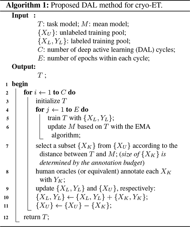
|
2.1. Pipeline of the Proposed Method
Notation.
We denote an unlabeled pool with and a labeled pool with , which is initially empty. Active learning is to select data from for annotation and to add the newly annotated data to , which is used to train the task model. The number of selected samples is determined by a given annotation budget. We use to denote the task model and the feed-forwarding operation. and denote the mean model and its feed-forwarding operation, respectively. For the other notations, we follow the definitions in Algorithm 1.
Data Selection.
For each unlabeled sample , we compute as the uncertainty for , where denotes a certain distance metric, such as MSE or KL divergence. We select unlabeled data of higher value for annotation. In fact, this selection scheme aims to pick out the data which leads to a higher deviation of output posteriors. We leave a discussion of its rationale in Section 2.2.
The Mean Model and EMA.
Exponential moving average (EMA) imposes greater significance on recent data and less significance on earlier data. This can be easily achieved by using a smoothing coefficient. [16] pioneered to apply the EMA technique in deep learning research. We denote the weights of with , and compute the weights of using
| (1) |
where refers to a training step and denotes the smoothing coefficient. We use for all the experiments.
In our method, the architecture of the mean model is exactly the same as that of the task model . The weights of can be obtained using Eq. (1). As a result, does not need to be trained in the whole DAL procedure, leading to a high efficiency of the proposed method.
Regularizer to Task Loss.
Unfortunately, data of higher deviation may result in poor generalization of the task model due to over-fitting. To mitigate this issue, we propose to use as a regularizer to the task loss, aiming to reduce the deviation introduced by newly annotated data. As a result, the entire loss function of the task model can be written as
| (2) |
where is an empirical loss (e.g. cross-entropy loss in classification) and is a trade-off coefficient. We choose unlabeled data of higher during data selection but minimize for labeled data during the task model training. Therefore, such a fashion to some extent can be regarded as “adversarial”. Since the model will not be trained, minimizing Eq. (2) only updates the model to make it approach , leading to a reduced deviation for the labeled data . This helps to mitigate overfitting and enhance the generalization of .
The Distance .
There are multiple options for the distance metric , such as MSE over feature space and KL divergence over output posteriors. In our method, has two modalities. Specifically, during data selection, we choose the KL divergence as over the posteriors of the two model outputs. Then the uncertainty of can be reformulated as
| (3) |
where denotes the softmax computation. During the task model training, we choose as over the output logits before softmax. Then Eq. (2) can be rewritten as
| (4) |
We observe that such a setting of yields the best performance, and provide an experimental analysis of in the ablation study.
2.2. Why Our Method Works
The rationale of a DAL method can be interpreted from two aspects, namely data selection and task model training. Here, we discuss the rationale of our method from these two aspects. Deviation-based Data Selection. This type of schemes have been demonstrated very effective in traditional active learning [17, 18, 19]. However, little work has managed to extend it for DAL. In addition, the deviation in a dataset is widely acknowledged to be capable of reflecting data uncertainty, but it fails to take task model into consideration. As illustrated in Eq. (3), for unlabeled data, our method evaluates how its posterior deviates from its average posterior (obtained from the mean model). Therefore, our method takes into account both data and task model, leading to a more accurate uncertainty estimation in the DAL context.
3. EXPERIMENT
We evaluate our method using three simulated and one real cryo-ET datasets. We compare our method with the state-of-the-art DAL baselines on the classification task. Given an unlabeled pool, we follow a common practice to randomly select 10% of the data for annotation and use it as the initial labeled data, which is kept the same for all the methods. We run each experiment for 3 trials and report the mean results. We refer readers to Appendix 1.1 for the training details, and Appendix 1.2 for an analysis of time efficiency.
3.1. Cryo-ET Datasets
Simulated Data.
We follow [20] to prepare the simulated data. All the simulated datasets consist of 50 classes but with three different SNRs (i.e. infinity, 0.05, and 0.03), leading to three datasets. A SNR of infinity is equivalent to “noise-free”. Each dataset includes 24000 training and 1000 testing samples, uniformly distributed across 50 classes. Each sample is a subtomogram, which is a 3D subimage of a tomogram that is likely to contain a single macromolecule.
Real Data.
The real cryo-ET data [21, 22] is collected from medical practices. The dataset consists of 4318 training samples and 1080 testing samples, distributed across 10 classes. It is a highly imbalanced dataset. For the training data, the number of samples in each class varies from 320 to 876. For the testing data, such a number varies from 80 to 219.
3.2. Classification Performance
Model Selection.
For the task model, we customize the original ResNet-18 [23] with 3D operations (e.g. 3D convolutions) to fit the cryo-ET input that is 3D grey scale image. We utilize the same architecture for the mean model, but its weights will not be updated via gradient descent. Both models are randomly and independently initialized. We use the same task model for all the compared methods for fair comparison.
Results and Analysis.
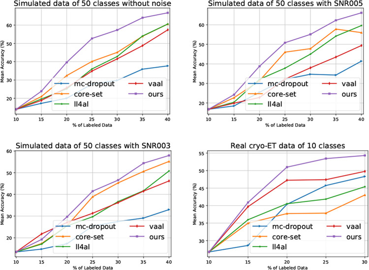
We compare our method with typical DAL baselines, including mc-dropout [13], core-set [15], vaal [8], and ll4al [4]. As illustrated in Fig. 1, our method outperforms the others on all the datasets. In addition, we have the following observations. Firstly, for almost each labeling budget, our method yields higher accuracy, demonstrating its reliability. Secondly, the real cryo-ET dataset is highly imbalanced and the superior performance demonstrates our method’s robustness to imbalanced data. Lastly, as the noise level increases (i.e. SNR005 to SNR003), our method still yields better results, demonstrating its robustness to noise.
Fig. 1.
Performance comparison between our method and the state-of-the-art DAL baselines on the cryo-ET datasets.
3.3. Ablation Study
Distance Metric.
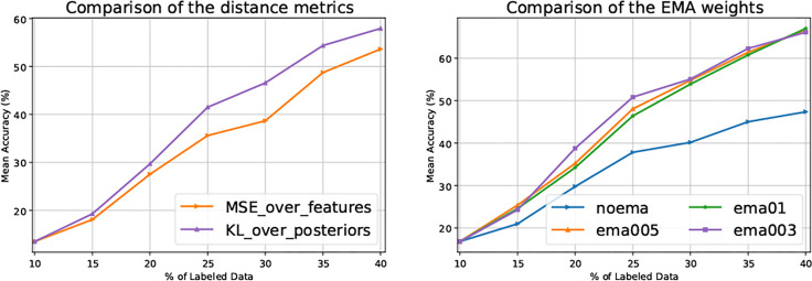
As shown in Eq. (3), we use the KL divergence as over the output posteriors to estimate uncertainty for unlabeled data. Here, we investigate what if MSE is used over output logits for uncertainty estimation. As illustrated in Fig. 2 Left, the KL divergence yields much better results, suggesting that the metric should be used over output posteriors rather than over output logits for uncertainty estimation. However, for the regularizer in Eq. (4), we observe that employing MSE as over output logits yields a better performance.
Fig. 2.
Left: Comparison of the distance metrics on the 50-class simulated dataset with a SNR of 0.03; Right: Comparison of the trade-off coefficients ( in Eq. (4)) on the 50-class simulated dataset with a SNR of 0.05.
Effect of the Regularizer.
As shown in Eq. (4), we propose to use a regularizer to reduce the deviation introduced by newly annotated data. In Fig. 2 Right, we study the trade-off coefficient . As can be seen, the performance is severely degraded when the regularizer is not used (i.e. , namely noema in the figure). For the other values, the results are slightly different. At the last cycle (i.e. annotation budget of 40%), the results are very close, indicating that there is no need of an extra effort to fine-tune this hyper-parameter. We use in all the experiments of our method.
Semi-Supervised Fashion.
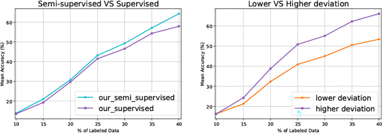
Till now, the regularizer in Eq. (4) only takes as input labeled data. Since the computation of MSE in Eq. (4) does not have to rely on label information, the regularizer can also work with unlabeled data, naturally leading to a semi-supervised fashion, even though can only be computed with labeled data. As shown in Fig. 3 Left, the semi-supervised version of our method further improves the task model performance, demonstrating the scalability of our method. Note that we conduct all the other experiments of our method in supervised fashion only, aiming at fair comparisons with the DAL baselines.
Fig. 3.
Left: The performance of our method and its semi-supervised version on the 50-class simulated dataset with a SNR of 0.03; Right: Comparison between selecting data of lower deviation and selecting that of higher deviation. This experiment is conducted on the 50-class simulated dataset with a SNR of 0.05.
Lower vs Higher Deviation.
As discussed in Section 2.1, we select unlabeled data of higher deviation for annotation. Here, we investigate what if data of lower deviation is selected for annotation. As shown in Fig. 3 Right, selecting data of higher deviation yields superior results. This observation also validates the rationale of our data selection scheme.
Number of Classes.
To explore how the number of classes in a dataset impacts our method performance, we run experiments on the simulated datasets of 10 and 50 classes, respectively. We compare the final accuracy at the last cycle (i.e. annotation budget of 40%), and show the performance improvement in Fig. 4. As illustrated, our method outperforms the others by a larger margin on the 50-class datasets than on the 10-class datasets, regardless of noise levels (i.e. SNR003 or SNR005), demonstrating the superiority of our method on datasets that consist of more classes.
Fig. 4.
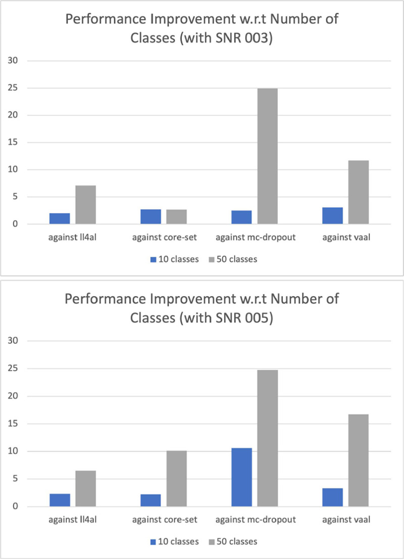
The performance improvement of our method over the others on the 10-class and 50-class simulated datasets. Top: With a SNR of 0.03 for both datasets; Bottom: With a SNR of 0.05 for both datasets.
4. CONCLUSION
In this paper, we propose a deviation based scheme for unlabeled data selection in deep active learning, highly applicable to cryo-ET challenges. To reduce the deviation incorporated by newly annotated data, we propose a regularizer for the task model training, leading to enhanced generalization. We unify the data selection and the task model training in a deep active learning framework and interpret its rationale based on the dropout and the deviation theories. We also show that our method can be easily extended to a semi-supervised fashion. Experimental results demonstrate the efficacy and efficiency of our method on both simulated and real cryo-ET data.
Acknowledgements
This work was supported in part by U.S. NSF grants DBI-1949629, IIS-2007595, and MCB-2205148, NIH grants R01GM134020 and P41GM103712, and Mark Foundation for Cancer Research 19-044-ASP. The computational resources were supported by AMD COVID-19 HPC Fund. XZ was supported in part by a fellowship from Center of Machine Learning and Health at Carnegie Mellon University. WW and BL were supported in part by the Microsoft AI4Earth grant.
5. REFERENCES
- [1].Gubins I, van der Shot G, Veltkamp RC, Foerster F, Du X, Zeng X, et al. , “Shrec’19 track: Classification in cryo-electron tomograms,” in Proceedings of the 12th EG Workshop 3D Object Retrieval, 2019. [Google Scholar]
- [2].Chen Muyuan, Dai Wei, Sun Stella Y, Jonasch Darius, He Cynthia Y, Schmid Michael F, Chiu Wah, and Ludtke Steven J, “Convolutional neural networks for automated annotation of cellular cryo-electron tomograms,” Nature Methods, vol. 14, no. 10, pp. 983, 2017. [DOI] [PMC free article] [PubMed] [Google Scholar]
- [3].Moebel Emmanuel, Martinez-Sanchez Antonio, Lariviere Damien, Fourmentin Eric, Ortiz Julio, Baumeister Wolfgang, and Kervrann Charles, “Deep learning improves macromolecules localization and identification in 3d cellular cryo-electron tomograms,” bioRxiv, 2020. [Google Scholar]
- [4].Yoo Donggeun and Kweon In So, “Learning loss for active learning,” in Proceedings of the CVPR, 2019, pp. 93–102. [Google Scholar]
- [5].Caramalau Razvan, Bhattarai Binod, and Kim Tae-Kyun, “Sequential graph convolutional network for active learning,” in Proceedings of the CVPR, 2021, pp. 9583–9592. [Google Scholar]
- [6].Du Xuefeng, Wang Haohan, Zhu Zhenxi, Zeng Xiangrui, Chang Yi-Wei, Zhang Jing, Xing Eric, and Xu Min, “Active learning to classify macromolecular structures in situ for less supervision in cryo-electron tomography,” Bioinformatics, vol. 37, no. 16, pp. 2340–2346, 2021. [DOI] [PubMed] [Google Scholar]
- [7].Zhang Beichen, Li Liang, Yang Shijie, Wang Shuhui, Zha Zheng-Jun, and Huang Qingming, “State-relabeling adversarial active learning,” in Proceedings of the CVPR, 2020, pp. 8756–8765. [Google Scholar]
- [8].Sinha Samarth, Ebrahimi Sayna, and Darrell Trevor, “Variational adversarial active learning,” in Proceedings of the ICCV, 2019, pp. 5972–5981. [Google Scholar]
- [9].Ducoffe Melanie and Precioso Frederic, “Adversarial active learning for deep networks: a margin based approach,” arXiv Preprint arXiv:1802.09841, 2018. [Google Scholar]
- [10].Kingma Diederik P and Welling Max, “Auto-encoding variational bayes,” arXiv Preprint arXiv:1312.6114, 2013. [Google Scholar]
- [11].Kipf Thomas N and Welling Max, “Semi-supervised classification with graph convolutional networks,” in Proceedings of the ICLR, 2017. [Google Scholar]
- [12].Gal Yarin and Ghahramani Zoubin, “Dropout as a bayesian approximation: Representing model uncertainty in deep learning,” in Proceedings of the ICML, 2016, pp. 1050–1059. [Google Scholar]
- [13].Gal Yarin, Islam Riashat, and Ghahramani Zoubin, “Deep bayesian active learning with image data,” in Proceedings of the ICML, 2017, pp. 1183–1192. [Google Scholar]
- [14].Kuo Weicheng, Christian Häne Esther Yuh, Mukherjee Pratik, and Malik Jitendra, “Cost-sensitive active learning for intracranial hemorrhage detection,” in Proceedings of the MICCAI, 2018. [Google Scholar]
- [15].Sener Ozan and Savarese Silvio, “Active learning for convolutional neural networks: A core-set approach,” in Proceedings of the ICLR, 2018. [Google Scholar]
- [16].Tarvainen Antti and Valpola Harri, “Mean teachers are better role models: Weight-averaged consistency targets improve semi-supervised deep learning results,” arXiv preprint arXiv:1703.01780, 2017. [Google Scholar]
- [17].Zidek James V and van Eeden Constance, “Uncertainty, entropy, variance and the effect of partial information,” Lecture Notes-Monograph Series, pp. 155–167, 2003. [Google Scholar]
- [18].Ji Ming and Han Jiawei, “A variance minimization criterion to active learning on graphs,” in AISTATS. PMLR, 2012, pp. 556–564. [Google Scholar]
- [19].Yang Yazhou and Loog Marco, “A variance maximization criterion for active learning,” Pattern Recognition, vol. 78, pp. 358–370, 2018. [Google Scholar]
- [20].Liu Sinuo, Ma Yan, Ban Xiaojuan, Zeng Xiangrui, Nallapareddy Vamsi, Chaudhari Ajinkya, and Xu Min, “Efficient cryo-electron tomogram simulation of macromolecular crowding with application to sars-cov-2,” in Proceedings of the BIBM. IEEE, 2020, pp. 80–87. [Google Scholar]
- [21].Noble Alex J, Dandey Venkata P, Wei Hui, Brasch Julia, Chase Jillian, Acharya Priyamvada, Tan Yong Zi, Zhang Zhening, Kim Laura Y, Scapin Giovanna, et al. , “Routine single particle cryoem sample and grid characterization by tomography,” Elife, vol. 7, pp. e34257, 2018. [DOI] [PMC free article] [PubMed] [Google Scholar]
- [22].Guo Qiang, Lehmer Carina, Martínez-Sánchez Antonio, Rudack Till, Beck Florian, Hartmann Hannelore, Pérez-Berlanga Manuela, Frottin Frédéd eric, Hipp Mark S, Hartl F Ulrich, et al. , “In situ structure of neuronal c9orf72 poly-ga aggregates reveals proteasome recruitment,” Cell, vol. 172, no. 4, pp. 696–705, 2018. [DOI] [PMC free article] [PubMed] [Google Scholar]
- [23].He Kaiming, Zhang Xiangyu, Ren Shaoqing, and Sun Jian, “Deep residual learning for image recognition,” in Proceedings of the CVPR, 2016, pp. 770–778. [Google Scholar]


