A New Reaction for Improved Calibration of EPR Rapid-Freeze Quench Times: Kinetics of Ethylene Diamine Tetraacetate (EDTA) Transfer from Calcium(II) to Copper(II)

Abstract

The kinetics of the transfer of the chelate, ethylenediamine tetraacetate (EDTA), from Calcium(II) to Copper(II) in imidazole (Im) buffers near neutral pH, corresponding to the conversion, [Cu(II)Im₄]²⁺→ [Cu(II)EDTA]²⁻, are characterized with stopped-flow absorption spectroscopy and implemented as a tool for calibrating the interval between mixing and freezing, the freeze-quench time (t_Q), of a rapid freeze-quench (RFQ) apparatus. The kinetics of this reaction are characterized by monitoring changes in UV–visible spectra (300 nm) due to changes in the charge-transfer band associated with the Cu²⁺ ions upon EDTA binding. Stopped-flow measurements show that the rates of conversion of the Cu²⁺ ions exhibit exponential kinetics on millisecond time scales at pH values less than 6.8. In parallel, we have developed a simple but precise method to quantitate the speciation of frozen solution mixtures of [Cu(II)(EDTA)]²⁻ and tetraimidazole Cu(II) ([Cu(Im)₄]²⁺) in X-band EPR spectra. The results are implemented in a simple high-precision ‘recipe’ for determining t_Q. These procedures are more accurate and precise than the venerable reaction of aquometmyoglobin with azide for calibrating RFQ apparatus, with the benefit of avoiding high-concentrations of toxic azide solutions.

1. Introduction

Rapid-Freeze-Quench (RFQ) techniques provide a method to determine the kinetics of formation of reaction intermediates and to characterize those intermediates with spectroscopic techniques that are not amenable to stopped-flow technologies. Advances in methodology and the convenience of commercially available apparatus have greatly expanded this approach. In general, the most common system used to calibrate mixing/quenching times in RFQ systems is the kinetics of binding of azide (N₃⁻) to aquometmyoglobin (metMb) [1–4]. The progress of that reaction can be monitored by numerous techniques (e.g., EPR, Raman, Mossbauer); for example, it is easily measured via stopped-flow absorption due to changes in the Soret band upon azide binding. For EPR, frozen-solution EPR spectra of the high-spin (HS) (S = 5/2) iron Fe(III) in aquometmyoglobin (metMb) exhibits a characteristic axial-EPR spectrum (g_⊥ = 6.0, g_∥ = 2.0) while the EPR spectrum for the low-spin (LS) (S = 1/2) metMbN₃ complex is rhombic with g = (2.82, 2.22, 1.73). The kinetics can be monitored by measuring the peaks heights of the g = 6 feature from the high-spin Mb and either the g₁ = 2.82 or the g₂ = 2.22 features of the low-spin MbN₃ complex, and thereby used to calibrate the interval between mixing and freezing, the freeze-quench time (t_Q), of an RFQ apparatus.

Though use of the metMb/azide reaction for calibration, testing, and training has a long and successful history, the toxicity of azide solutions causes practical storage and disposal issues in modern laboratories. This problem is amplified when calibrating an RFQ apparatus, especially working on an extremely short time scale. It can often take multiple samples to achieve a single consistent t_Q, which must be repeated for multiple configurations of the RFQ apparatus when characterizing the kinetics of formation of an intermediate. Beyond that, we show here that the quantitation of the metMb/azide reaction extent suffers from intrinsic weaknesses that are overcome by the procedures described here.

This work began with an effort to develop a new calibration reaction(s) that achieves comparable experimental utility and occurs on the same timescale as that for azide binding to metMb, that was convenient to apply in ordinary CW EPR spectroscopy at X-band, yet avoided the need for toxic solutions of azide, We note that Potapov and Goldfarb [5] reported an alternative azide-free EPR calibration reaction that could be used at X-band only with pulsed EPR, and was developed to calibrate RFQ with higher microwave frequencies, in particular W-Band (94 GHz).

As a benchmark for the rate of reactions that are required, we took the pseudo-first order rate constant of 25 s⁻¹ for a 10 mM azide solution reacting with solution of 1 mM metMb at pH 7.8 [1], which gives an approximate t_1/2 of 30 ms. We here describe the use of the ubiquitous chelate, ethylenediamine tetraacetate (EDTA), and its reaction with Cu²⁺. The reaction of H_nEDTAⁿ⁻⁴ with Cu²⁺ is too fast (second order rate constant 1.3 × 10⁹ M⁻¹ s⁻¹ at 25 °C) [6] to provide a calibration reaction. However, because Cu²⁺ has one of the highest affinities (binding constant, K) of all + 2 metal ions for the EDTA ligand (log(K) > 18), [7] mixtures of [M(II) (EDTA)]²⁻ and thus the [Cu(II)(Im)₄]²⁺ present in imidazole buffers will quantitatively evolve to [Cu(II)(EDTA)]²⁻ over time, corresponding to the EPR-observable conversion,

$${[\text{Cu}(\text{II}){(\text{Im})}_4]}^{2+}\to {[\text{Cu}(\text{II})\text{EDTA}]}^{2-}$$

In such a reaction, the off-rate of the ligand from the M(II) will determine the effective rate of formation of [Cu(II)(EDTA)]²⁻. We restricted the possible choices of metal ions to those that are (A) air stable to oxidation for ease of sample preparation and handling and (B) EPR-inactive for easier analysis, and (C) non-toxic. Tests of multiple such ions led us to focus on Ca²⁺and Zn²⁺, log(K) = 10.6 and 16.4, respectively [7], ultimately choosing the former. Through calibration with stopped-flow optical spectroscopy, we found that the reaction of solutions of the complex [Ca(II)(EDTA)]²⁻ (CaL²⁻) with Cu²⁺ in imidazole buffers near neutral pH have appropriate kinetic properties for testing and calibration of RFQ-EPR systems, while we show that the EPR changes seen in the RFQ-samples that result from this reaction are readily quantitated with high precision. This reaction not only provides an excellent and non-hazardous alternative to the metMb/azide system, but also one we show to be more accurate. In this paper, we detail the development and procedures for usage of the ‘Cu-calibration’ procedure, culminating with the presentation of a ‘simple recipe’ for determining the t_Q of any particular configuration of a freeze-quench apparatus.

2. Experimental

Depending on the pH required, buffers were prepared with 50 mM imidazole and 100 mM of either 2-(N-morpholino)ethanesulfonic acid (MES) or 3-(N-morpholino) propanesulfonic acid (MOPS). Sufficient NaCl was added to bring the ionic strengths (I) to 0.15 M. The pH was measured with Beckman/Coulter pHi 510 at ambient conditions. Imidazole (Aldrich), MES monohydrate (Alfa Aesar), MOPS sodium salt (DOT Scientific), CaCl₂·2H₂O (Sigma), CuCl₂·2H₂O (Aldrich), ZnSO₄·7H₂O, (EM Industries), disodium ethylenediamine tetraacetate (BDH) were used without further purification. Solutions were prepared in MilliQ purified water using standard precision volumetric techniques.

UV–visible spectra were acquired on an Agilent 8413 at ambient conditions using a 1.00 cm quartz cuvette. Stopped flow optical absorption spectra were taken with an Applied Photophysics SX-17 with a xenon arc lamp source that was equipped with an Applied Photophysics photomultiplier tube detector. The path length of the cell was 1.00 cm.

All EPR spectra were collected on a Bruker ESP-300 equipped with TE-102 resonator; temperature was controlled and monitored with an Oxford ESR-900 cryostat and Oxford Mercury ITC controller. Data acquisition was performed with locally constructed software using National Instruments multifunction DAQ hardware. EPR spectra were recorded at 30 K. Each spectrum consists of 2048 points across the field range of 240.0–360.0 mT. Scan rates were 1.0 mT/s (120 s/scan) and 4 scans were averaged. Microwave power (2.0 mW), time constant (160 ms), modulation amplitude (0.60 mT), receiver gain (5.0 × 10⁴) were kept constant for all measurements. The microwave frequencies were measured with an EIP 548A counter and were in the range 9.360–9.365 GHz for all samples.

RFQ samples were prepared using an Update Instruments model 715 equipped with the commercial mixer. The reaction mixture was quenched by spraying onto two rotating aluminum wheels cooled to liquid nitrogen temperatures as previously described [3, 8]. The frozen powder was collected in a funnel and packed into standard 4 mm OD X-band EPR tubes. RFQ- EPR samples were annealed in a dry ice-methanol bath for 5 + minutes to remove as much frozen air as possible. A tamping rod held the sample in place during the annealing process.

3. Kinetics Model

In the buffer/imidazole solutions employed, with high concentrations of imidazole relative to Cu²⁺ concentrations, Cu²⁺ is present as the complex tetraimidazole Cu(II), [Cu(II)(Im)₄]²⁺ (Cu(Im)₄²⁺). We use a simplified model for the rate of formation of the complex [Cu(II)(EDTA)]²⁻ (CuL²⁻) from a mixture of [Ca(II)(EDTA)]²⁻ (CaL²⁻) and Cu²⁺ in imidazole (Im) buffer solutions on the two-step process based on the two on-rates of EDTA ligand to (k₁ and k₂) to the Ca²⁺ and Cu²⁺ ions respectively, and the two off-rates of EDTA ligand from their respective complexes (k₋₁ and k₋₂):

$$\begin{gathered} \text{n}({\text{BH}}^{+})+{\text{CaL}}^{2-}\underset{k_1}{\overset{k_{-1}}{\rightleftarrows }}{\mathrm{H}}_{\text{n}}{\text{L}}^{n-4}+{\text{Ca}}^{2+} \\ {\mathrm{H}}_{\text{n}}{\text{L}}^{n-4}+\text{Cu}{\left(\text{Im}\right)}_4^{2+}\underset{k_{-2}}{\overset{k_2}{\rightleftarrows }}{\text{CuL}}^{2-}+\text{n}({\text{BH}}^{+}) \end{gathered}$$ (1)

where B is buffer (either imidazole or the co-buffer). The off-rate for CuL²⁻ (k₋₂) under the experimental conditions in this paper was found to be 5 × 10^–3 s⁻¹ (details in SI) and therefore can be ignored on time scales below 1 s. We apply the steady-state approximation for the free ligand (H_nLⁿ⁻⁴) and make the testable hypotheses that k₋₁ < < k₁ = k₂ and solve for the fraction of total Cu²⁺ that is bound to EDTA (fr_E) as a function of time

$$f{r}_E(t)=\frac{1-\text{exp(−}{k}^{\prime }t\text{)}}{1-R^{-1}\text{exp}(-k^{\prime }t)};k^{\prime }=(R-1)[{({BH}^{\text{+}}]}^n{k}_{-1}$$ (2)

where R is the ratio of the initial CaL²⁻ concentration to the initial Cu²⁺ concentration ([CaL²⁻]₀/[Cu²⁺]₀) and R > 1[9] We are using the second-order integrated rate law rather than the simplified pseudo-first order solution as the range of R values studied is not large enough to justify the assumptions of pseudo-first order kinetic behavior.

As a method of testing the hypothesis that the on-rate of EDTA to Ca²⁺ (k₁) is equal to the on-rate of EDTA to Cu²⁺ (k₂), we employed solutions with excess Ca²⁺ as a technique of slowing the rate of the formation of CuL²⁻. We employ a simplified notation, R×C, to denote a solution that where the ratio of [CaL²⁻]₀/[Cu²⁺]₀ is R and the ratio of excess [Ca²⁺]₀/[Cu²⁺]₀ is C. Therefore, when reacted in equal volumes with a 1.00 mM Cu²⁺ solution, a solution that is 6.00 mM in Ca²⁺ and 4.00 mM EDTA contains 4.00 mM CaL²⁻, 2.00 mM excess Ca²⁺, so this solution is denoted 4 × 2.

Under the conditions of excess Ca²⁺, we get the same time course described above but the observed rate constant becomes

$$k^{\prime }=\left(\frac{R-1}{C+1}\right)k_{\text{off}}:k_{\text{off}}={[{(BH)}^{+}]}^n{k}_{-1}$$ (3)

At a given pH, plotting k′ versus (R − 1)/(C + 1) for a set of CaL²⁻/Ca²⁺ solutions that vary R and C will have a slope of k_off = [(BH⁺)]ⁿk_−1, which we take to be the effective off-rate of EDTA from Ca²⁺ at that pH. Details of the derivations of Eqs. (2) and (3) are given the SI.

4. Developing the Kinetics of the [Cu(II)(Im)₄]²⁺→ [Cu(II)(EDTA)]²⁻ Conversion

4.1. UV–Visible Spectra

The [Cu(II)(EDTA)]²⁻ complex has an intense ligand-to-metal charge transfer band in the UV region that can be monitored to follow the course of the reaction [10]. Electronic spectra recorded from 250 to 400 nm of a titration in which aliquots of CaL²⁻ were added to 0.50 mM Cu²⁺ in 100 mM MES, 50 mM Im (MES/Im) buffer at pH 6.50 are shown in Fig. 1 (ambient temperature (23 °C)). The absorbance at 300.0 nm rises linearly from 0.119 (ε = 238 M⁻¹ cm⁻¹) to 0.674 (ε = 1350 M⁻¹ cm⁻¹) as the concentration of CaL²⁻ is increased from 0.00 to 0.50 mM. We have chosen 300.0 nm for the wavelength to monitor as it is the shortest wavelength for observation that is available on our stopped-flow system.

Fig. 1.

UV–Visible spectra from 250–400 nm of titration of Ca(EDTA)²⁻ into 0.50 mM Cu²⁺ in 100 mM MES/50 mM imidazole at pH 6.50. Inset: a plot of the absorbance at 300 nm vs μM of Ca(EDTA)²⁻ showing that the change at this wavelength is directly related to the fraction of [Cu(II)(EDTA)]²⁻ complex in the mixture. Ambient temperature (23 °C)

4.2. Stopped-Flow of Calcium-EDTA/ Cu(II) Kinetics

All stopped-flow absorption experiments were done using equal volumes of 1.00 mM Cu²⁺ solutions and R×C solutions of CaL²⁻/Ca²⁺ in at a given pH in buffers described above. With the exception of the temperature dependence, all measurements were done at 23.0 °C. Single wavelength kinetic measurements were observed at 300.0 nm. All time traces represent a linear array of 1000 time points across the given time scale.

The time traces were fit using non-linear least squares procedure to extract three terms (A₀, ΔA, k′) given the value of R in the CaL²⁻/Ca²⁺ mixture.

$$A(t)=A_0+\Delta Af{r}_E(t;R):f{r}_E(t;R)=\left(1-\text{exp}(-k^{\prime }t)\right)/\left(1-R^{-1}\text{exp}(-k^{\prime }t)\right)$$ (4)

Here, A₀ is the absorbance of 0.50 mM Cu(Im)₄²⁺ in the buffer at 300 nm, ΔA is the absorption difference between 0.50 mM CuL²⁻ and 0.50 mM Cu(Im)₄²⁺ in the given buffer at 300 nm, and k′ is the observed rate constant. The values of A₀ and ΔA are allowed to vary to compensate for small differences in concentrations or slight changes in properties that might to due to the small deviations in the pH of the solutions.

4.2.1. Dependence of Rate of Reaction on pH

A series of buffers from pH = 6.50–7.55 were prepared. In each buffer, mixtures of 4.00 mM CaL²⁻ + 2.00 mM Ca²⁺ (4 × 2) was reacted with an equal volume of 1.00 mM Cu²⁺ in the same buffer solution and the time course of the reaction monitored at 300.0 nm at 23 °C. The rate of the reaction is strongly dependent on pH as shown in Fig. 2. At pH 7.55, the reaction is complete in ~ 10 s where at pH 6.50 the reaction is complete in less the 0.5 s. Best-fit parameters, including the rateconstants, k’ are listed in Table S1. A plot of log(k′) vs pH gives a straight line with slope = − 1.4, corresponding to an increase in the rate of the reaction of approximately 25-fold by lowering the pH by 1 unit.

Fig. 2.

pH dependence of the rates of the transfer of EDTA from [Ca(II)(EDTA)]²⁻ to Cu²⁺ in 100 mM MOPS/50 mM imidazole or 100 mM MES/50 mM imidazole buffers. Single wavelength stopped-flow measurement at absorbance at 300 nm. Each time trace consists of 1000 time points taken over the relevant total time period. Each reaction consists of a mixture of 6.00 mM Ca²⁺, 4.00 mM EDTA (4 × 2) reacted with an equal volume of 1.00 mM Cu²⁺ in the given buffer system. The inset details a log plot of the best fit k′ vs pH. Temperature was held constant at 23.0 °C for all measurements

The simple kinetics model described above successfully fits the time dependence at all pH values but shows systemic errors for pH values above pH = 7.0 and the extent of the errors increases as the pH increases between 7.00 and 7.55 as shown by the increasing χ² (sum square of residuals) of the fit. The least-squares fit to the simple model predicts a much slower early phase of the experiment (fit curve below experiment) than is observed which then crosses (fit curve above experiment) at longer times to compensate. An example is shown in Fig. S4.1. This shows that at the higher pH values, the reaction does not obey single-exponential behavior. This same behavior is observed in other CaL²⁻/Ca²⁺ mixtures in this pH range. The nature of this breakdown of the simple kinetics model is beyond the scope of this paper. Because the kinetics in the lower pH range comport to our simple model, we chose the single buffer system of 100 mM MES, 50 mM imidazole at pH = 6.50 and I = 0.15 M for all other measurements.

4.2.2. Rates of Reactions at pH 6.50, 23.0 °C

A set of solutions CaL²⁻ with excess Ca²⁺ ranging from 5 × 1 (fastest) to 3 × 3 (slowest) were prepared in MES/Im at pH 6.50 and the absorbance was monitored at 300.0 nm. The absorbance data were fit using the procedure described above and the best-fit results are summarized in Table S2. A plot of the k′ vs. (R − 1)/(C + 1), Fig. 3, gives a straight line with slope 15.0 s⁻¹. The linear dependence of the observed rate on the value of (R − 1)/(C + 1) confirms the assumption that the on-rates of EDTA to Ca²⁺ (k₁) and Cu²⁺ (k₂) are effectively equal under this set of conditions. The slope of the line is the effective off-rate of EDTA from Ca²⁺ at the given pH, k_off of Eq. (3). We also have found that using excess Ca²⁺ in the solutions has an additional benefit of ensuring that there is no ‘free’ EDTA that might be the result of slight errors in sample preparation when attempting to make exactly 1:1 Ca²⁺/EDTA in the solutions.

Fig. 3.

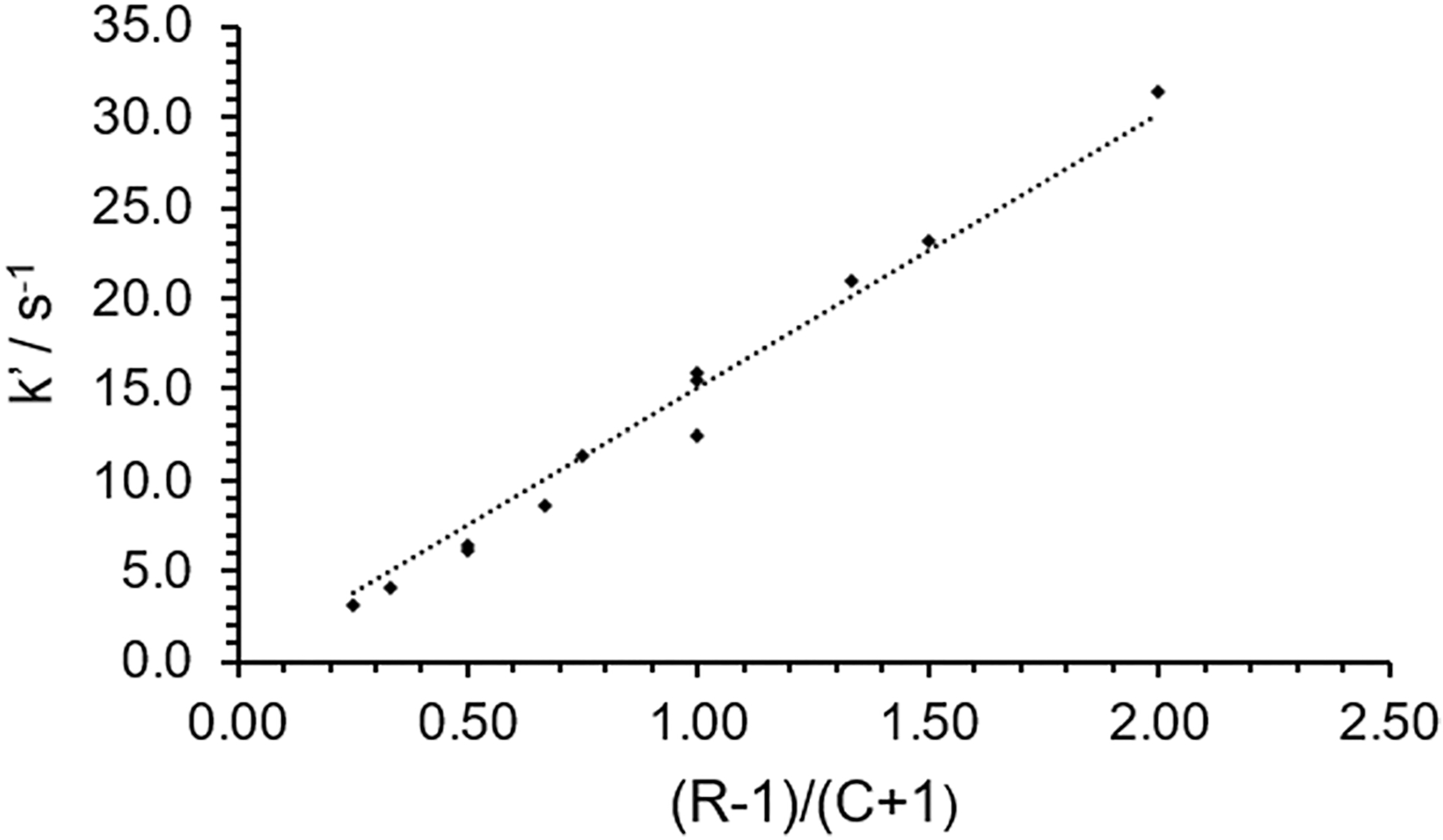
Plot of best-fit k′ vs the reaction mixture ratio of (R − 1)/(C + 1) at pH 6.50 in MES/Im buffer at 23.0 °C. The straight-line shows that in this regime of concentrations in this buffer system, the on-rates of EDTA to Ca²⁺ and Cu²⁺ are similar. The trend line has a slope of 15 s⁻¹ which represents the effective off-rate of EDTA from Ca²⁺ (k_off) in this buffer system at this temperature

4.2.3. Temperature Dependence

At pH 6.52, stopped-flow absorption measurements were done across the temperature range from 13.7 °C to 27.9 °C (see Fig. S5.1). The results give an activation barrier of 78 kJ mol⁻¹. This predicts about a 12% change/°C in reaction rate in the temperature range around 23 °C. The release of EDTA from Ca²⁺ under these conditions, k_off = 15 s⁻¹, gives a t_1/2 of approximately 50 ms for reactions with the value of (R − 1)/(C + 1) of 1.0 (3 × 1, 4 × 2, 5 × 3 etc.). The results of the stopped-flow absorption measurements thus demonstrate that the kinetics of the transfer of EDTA from [Ca(II)EDTA]²⁻ to [Cu(II)(Im)₄]²⁺ at pH 6.50 under the described conditions are in the range required for calibrating millisecond scale quench times (t_Q) for RFQ systems.

5. EPR Spectroscopy

5.1. Spectral Fitting Procedure

In this section, we show that we can precisely quantitate the fractions of the two Cu(II) complexes, [Cu(II)EDTA]²⁻ and [Cu(II)(Im)₄]²⁺, in EPR spectra of mixtures of these two species, both in frozen solution and in RFQ samples (packed powders). Figure 4 shows examples of normalized frozen-solution X-band EPR spectra of CuL²⁻ and Cu(Im)₄²⁺, obtained as described directly below. The spectra of these two Cu(II) complexes have significant spectral overlap and there are no simple features that can ‘eyeballed’ and utilized to extract the relative concentrations of the two species as can be done with the metMb-azide system. Nonetheless, the two spectra do have significant, readily quantitated, differences. For CuL²⁻, g_||= 2.30, A_||= 450 MHz and the perpendicular region of the spectrum is relatively narrow with an approximate g_⊥ of 2.07; for Cu(Im)₄²⁺, g_||= 2.26, A_||= 540 MHz and the perpendicular region is broader, shifted to higher field, g_⊥ = 2.055, and exhibits resolved ¹⁴ N hyperfine from the imidazole ligands. These apparently small differences in spin-hamiltonian parameters lead to the substantial difference in the numerical difference spectrum shown in Fig. 4.

Fig. 4.

Normalized frozen solution EPR spectra of 0.50 mM CuL²⁻ (red) and 0.50 mM Cu(Im)₄²⁺ (black) in MES/imidazole buffer at pH 6.50 and the normalized difference spectrum (CuL²⁻–Cu(Im)₄²⁺ blue dash). Details of normalization process given in text. Conditions as described in Experimental (Sect. 2)

To quantitate these differences, all collected EPR spectra are normalized to the same double integral by the following procedure:

1. The background spectrum of a frozen buffer solution is subtracted from the sample spectrum

2. The script described below corrects for a sloped baseline by averaging the first 10 points and the last 10 points of the Y and subtracting a line across the spectrum based on these two values. This step is carried out on all spectra but in fact is necessary only for RFQ samples, and there the influence is minimal.

3. The average of the Y array is subtracted.

4. The integral spectrum is calculated and checked for any systemic errors.

5. The value of the double integral (DI) is calculated and the derivative spectrum after step C is adjusted by a given scale value, in this case by 10,000/DI. (X-axis units in Gauss).

We denote the normalized Y array of each spectrum as S_Z, where Z is the unique identifier: E for CuL²⁻, Im for Cu(Im)₄²⁺, X for mixture. This normalization process ensures that we can analyze spectra with different spin concentrations. This is important as RFQ samples are frozen ‘snows’ that are physically packed into an EPR tube, and thus inevitably of different densities, yielding differing effective spin concentrations and EPR intensities. We note this process is nearly identical to that proposed by Cherepanov and de Vries[2] and very similar to that suggested by Pievo et al. [4] for the far more challenging task of improving the precision of quantitation in the metMb/azide system (see below).

To decompose the spectra of mixtures into components, we use the fact that there are only two EPR-detectable complexes in the sample, Cu(Im)₄²⁺ and CuL²⁻ and any mixture of CuL²⁻ and Cu(Im)₄²⁺ will generate a normalized spectrum (S_X) that is simply the weighted average of the two normalized component spectra, S_E and S_Im for CuL²⁻ and Cu(Im)₄²⁺ respectively.

$$S_X=f{r}_E{S}_E+f{r}_{Im}{S}_{Im}$$ (5)

Using the requirement that the fractions sum to 1.00 (fr_E + fr_Im = 1.00) and rearranging gives a simple 1-parameter linear equation for fr_E at each mixture

$$(S_X-S_{\text{Im}})=f{r}_E(S_E-S_{\text{Im}})$$ (6)

Therefore, a simple linear least-squares fit extracts the fr_E from the normalized experimental spectra of mixtures of CuL²⁻ and Cu(Im)₄²⁺. We first demonstrate the precision of this approach on static frozen solution mixtures of EDTA with 0.50 mM Cu²⁺ in MES/Im buffers, Fig. 5. In Sect. 5.2, we then apply this technique to freeze-quench reactions experiments where the value of fr_E(t) determines the extent of reaction and thereby the effective quench times.

Fig. 5.

Example of fitting procedure with sample that is 0.15 mM CuL²⁻ and 0.35 mM Cu(Im)₄²⁺. Top: Normalized frozen solution spectra of 100% Cu(Im)₄²⁺ (S_Im) (Black) and 30% CuL²⁻ + 70% Cu(Im)₄²⁺ (S_X) (Red). Bottom: Black, normalized experimental difference of (S_X−S_Im) compared with a 30% scaling of the normalized exemplar difference 0.3(S_E − S_Im) (red dashed)

Figure. 5 shows a simple system in which a solution that is 0.50 mM Cu²⁺ and 0.15 mM EDTA (fr_E = 0.30) in the pH 6.50 MES/Im buffer system is frozen and the EPR recorded at standard conditions. The normalized experimental spectrum (S_X) is shown in red and the normalized imidazole spectrum is shown in black in Fig. 5 top. The difference (S_X − S_Im) and 0.3(S_E − S_Im) is shown in Fig. 5 bottom. In this case, the best fit for fraction of CuL²⁻ is 0.297.

To facilitate use of this approach, we have automated the normalization and fitting method with a Python script that is provided in the SI.

5.1.1. Tests of the Procedure

We have tested this method on a series of frozen solutions of 0.50 mM Cu(II) in MES/Im buffers at pH 6.50 with values of fr_E ranging from 0.05 to 0.75. The normalized difference spectra are shown in Fig. S6.1. When applying the procedures detailed in Sect. 5.1 to each of the 9 spectra to obtain an EPR-determined fraction of EDTA-bound Cu(II) in the solution, we find that all but one fit gave a fraction of EDTA-bound Cu(II) that agreed with the actual value of fr_E = 0.15 to within 0.01. (Data given in Table S3). Given these results we employ a generous uncertain in fr_E ± 0.02 in analyses below.

The normalization and fitting procedure by which we determine the reaction extent, fr_E, was further tested by comparing the spectrum decomposition of a frozen solution prepared with 0.50 mM Cu²⁺ + 0.15 mM EDTA in MES/Im buffer, corresponding to fr_E = 0.30, to that of an RFQ sample prepared using the same in both syringes (a null reaction). This simple quick test ensures that the process of collecting and packing an RFQ sample does not compromise the accuracy or precision of the quantitation. In Fig. 6 (upper), we show a comparison of the ‘raw’ spectra after simple baseline subtraction of the frozen solution of this composition versus the same solution packed in an EPR tube after RFQ preparation. When the normalization process is applied to both spectra, the resulting normalized spectra are effectively identical as shown in Fig. 6 (lower). The double integrals of the two spectra show that effective spin concentration of the RFQ sample is approximately 50% of the frozen solution sample. The processing of these two spectra is shown in more detail in the supplement.

Fig. 6.

Comparison of EPR spectra of frozen solution (black) and RFQ hand packed sample (red) after simple baseline corrections and no normalization. Solution is 0.50 mM Cu(II), 0.15 mM EDTA in MES/Im buffer at pH 6.50. The relative double integral areas are approximately 2:1, so the packing density of the RFQ sample is approximately 50%. Bottom: Same spectra normalized by double integral. The blue line is the difference between the two normalized spectra

6. Application of the Cu(Im)₄→Cu(EDTA) Conversion to Determining t_Q in RFQ EPR

6.1. RFQ Kinetics

RFQ samples were prepared with different mixer conditions for samples generated with each of two different mixtures of CaL²⁻/Ca²⁺ solutions 5 × 1 and 5 × 2 (pH = 6.50 in MES/Im buffer) reacted with the [Cu(II)(Im)₄]² complex that forms upon the addition of Cu²⁺ to this same buffer, each reaction having been calibrated and its value for the conversion, k′ determined with stopped flow measurements. The calibration curves for the two mixtures are shown in Fig. 7. The quench times, t_Q, subsequent to mixing were then determined for each mixture with three different configurations of ageing-tube length and ram speed. For each configuration, a freeze-quench sample was collected for each mixture and its EPR spectrum taken. From this spectrum and the three reference spectra (background (buffer); Cu(Im)₄²⁺; CuL²⁻), the fractions of EDTA-bound Cu(II), the fr_E(t_Q) for each configuration of each solution were determined by simply running the script given in SI. Through use of Eq. (2), the script extracted the value of t_Q from the value of the rate constant, k’ for the reaction mixture, the initial ratio R, and the value of fr_E(t_Q) obtained in the analysis of the RFQ EPR spectrum,

$$\text{exp}(-k^{\prime }{t}_Q)=\frac{1-f{r}_E(t_Q)}{1-R^{-1}f{r}_E(t_Q)}:t_Q=-\frac{1}{k^{\prime }}\ln \left(\frac{1-f{r}_E(t_Q)}{1-R^{-1}f{r}_E(t_Q)}\right)$$ (7)

Fig. 7.

Plot of quench time versus fraction of CuL²⁻ formed during reactions of 1.00 mM Cu²⁺ reacted with 5.00 mM CaL²⁻ + 1.00 mM Ca²⁺ (5 × 1, black) and 5.00 mM CaL²⁻ + 2.00 mM Ca²⁺ (5 × 2, red) in MES/Im buffer pH 6.50. The dashed curves are calibrations obtained from stopped-flow absorption on these same samples. The points represent fr_E(t_Q) from EPR RFQ measurements of each sample using RFQ samples prepared with the three different mixer configurations listed in the text. Error bars in t_Q are determined by assuming the error in fr_E(t) to be ± 0.02

The measured fr_E and calculated t_Q are summarized in Table 1; the spectra and fits are shown in the supplement. The experimental points on Fig. 7 display the value of t_Q(fr_E) for each sample as determined from the measured fractions for the three RFQ configurations. The error limits in the quench times are determined by the statistical uncertainties in the fr_E of ± 0.02. As listed in Table 1 and displayed in Fig. 7, at modest levels of conversion, say 0.05 ≲ fr_E ≲ 0.75, the uncertainties in t_Q are truly insignificant; as the conversion of Cu2+ approaches completion by extending the quench time, the uncertainties associated with the quench times increase, but still remain quite small. Significantly, the values of quench times for the CaL²⁻/Cu²⁺ reactions for the two solutions are consistent with each other and this experiment demonstrates the simplicity and precision of this reaction and data processing method.

Table 1.

RFQ results for CaL²⁻/Cu²⁺ reactions

Solution mixture	RFQ configuration	Fraction reacted (frE)	χ 2	Calculated quench time
5×1	A	0.49	2.71×10−2	23 ± 1.5 ms
5×1	B	0.69	1.57×10−2	42 ± 2.5 ms
5×1	C	0.87	1.52×10−2	74 ± 6 ms
5×2	A	0.39	5.2×10−2	26 ± 0.5 ms
5×2	B	0.52	0.79×10−2	39 ± 2 ms
5×2	C	0.79	0.83×10−2	87 ± 6 ms

Summary of best-fit parameters of fraction CuL²⁻ (fr_E) in RFQ mixtures of CaL²⁻/Cu²⁺ in pH 6.50 MES/imidazole buffers at different quench times. Reactions were done at ambient conditions (23 °C). The three different configurations are detailed in the text. Error limits on quench times estimated from assuming ± 0.02 for fr_E. RFQ configurations: (A) 21 mm ageing tube, 6.5 cm/s, (B) 53 mm ageing tube, 6.5 cm/s, (C) 53 mm ageing tube, 1.6 cm/s

Significantly, we have found that the quench times measured with the metMb/azide reaction do not match those measured with the CaL²⁻/Cu²⁺ reactions. For the three configurations of the RFQ apparatus, a 5 mM azide solution reacted with a 1 mM metMb at pH 7.0, 23 °C yielded a quench time that in each case is approximately a factor of two shorter than the quench time measured with the CuL²⁻/Cu²⁺ reactions. Two major factors lead us to believe the ‘new’ reaction quench times are more accurate than the results of the standard reaction: (1) the rate constants for EDTA transfer for the CaL²⁻/Cu²⁺ reactions were verified by stopped-flow on the same solutions used for RFQ. (2) More important is the major and intrinsic weakness of the standard reaction: the quality of the EPR spectra using 0.50 mM Cu²⁺ samples is significantly better for quantitation than that for 0.50 mM metMb. The first disadvantage of the standard method is lower EPR signal intensity, which is firstly related simply to the criterion of spins/gauss, but secondly involves characteristics of the derivative EPR signal. The Cu²⁺ spectra cover a relatively narrow X-band total field range, from 260 to 340 mT, and both ‘reactant’ and ‘product’ Cu(II) complexes have derivatives with comparable peak-peak intensities. The second weakness is the difference in breadth and shapes of the derivative EPR spectra. The derivative EPR spectrum of the HS metMb covers the broad X-band field range of ~ 100–380 mT and it has an intense and narrow feature at approximately 120 mT and then continues with negligible intensity up to 360 mT; the g_|| feature is relatively weak and buried under the LS signal. The LS metMbN₃ spectrum has relatively broad derivative features across a field range from approximately 280–400 mT. In the ‘olden days’, when this method was initially devised and EPR spectra were recorded on paper, the large field range and separation of the features was a benefit. However, the large dynamic range in the Y (intensity) axis of the two derivative spectra combined with the wide field sweep required on the X axis creates baseline ‘roll’ that affects the precision of any double-integration-based method.

These baseline problems are exacerbated in RFQ samples, which tend to contain varying quantities of frozen O₂ that generate EPR signals in addition to the signals from the species of interest. The issues with the variable packing density and variable baselines were discussed in detail by Cherapanov and de Vries [2], and the magnitude of the problems they face is highlighted by the ‘raw’ spectra shown in their paper. They provide a detailed method for improving the quantitation the metMb/azide RFQ reactions that involves static mixtures and null RFQ reactions. We have chosen to change the reaction rather than the attempting to incrementally improve upon the method. Using the [Cu(II)(Im)₄]²⁺→[Cu(II)EDTA]²⁻ reaction, we find that the small effect of frozen O₂ on annealed RFQ samples is seamlessly removed by Step B in the procedure shown above. While the metMb/azide reaction has excellent properties for an optical experiment such as stopped-flow absorption, the issues addressed by de Vries and coworkers demonstrate that this reaction has poor properties for EPR quantitation. By switching to a reaction that is based upon Cu²⁺ EPR spectra, we have focused on the accuracy and precision of the EPR measurement first, and found that we did not need to sacrifice the accuracy and simplicity of the stopped-flow absorption measurements for the calibration of reaction rates.

6.2. Simple Recipe

We provide the following procedure that we use for determining the t_Q of an RFQ apparatus:

1. Prepare and record EPR spectra of three frozen solution static samples, 0.50 mM Cu²⁺ in pH 6.5 MES/Im buffer, 0.50 mM CuL²⁻ in pH 6.50 MES/Im buffer (best to use a small excess of EDTA), and third, pure buffer.

2. Select a R×C solution that yields a t_1/2 in the time range for t_Q you are expecting. In general, this is done by reference to Fig. 8. If higher precision is required, carry out a stopped flow measurement to determine k’ of reaction mixture(s). Input the values of k’ and R in the Python script.

3. Prepare pH 6.50 MES/Im buffer solutions of 1.00 mM Cu²⁺ as well as the R×C solution of CaL²⁻/Ca²⁺

4. Perform RFQ experiment and record EPR spectrum.

5. Edit script to provide pathways to the 4 spectra: background, Cu(Im)₄²⁺, CuL²⁻, and RFQ experiment.

6. Run script(

7. The script will output both extent of reaction (fr_E) and quench time (t_Q).

Fig. 8.

Measured or estimated t_1/2 for different reaction mixtures of R × C (R mM CaL²⁻ + C mM Ca²⁺) reacted with 1.00 mM Cu²⁺ in 100 mM MES/50 mM Im at 23 °C, pH 6.50. The # represent solutions where the k′ and t_1/2 calculated using Eq. (3) with k_off = 15 s⁻¹

7. Summary and Conclusions

The [Ca(II)(EDTA)]²⁻/[Cu(II)(Im)₄]²⁺ reaction has many attractive ‘practical’ features that recommend its use in testing and calibrating RFQ systems for EPR spectroscopy. Firstly of course, it does not use toxic azide solutions, but beyond that, the chemicals used are all solids with long shelf lives and require no special handling or disposal. Secondly, the use of this system enjoys the advantage that precisely the same solutions are used for both RFQ and stopped-flow absorption, thus yielding high-precision values for the rate constants k’ as a function of solution conditions. In contrast, the azide/metMb method employs optical and EPR solutions of widely different concentrations. Finally, the availability of modern data acquisition and analysis software makes, the analysis/calibration process of double-integration normalization both fast and precise, easily yielding high-precision values for the quench-times, t_Q, for each configuration of an RFQ apparatus. In contrast, it is a major challenge to accurately integrate and normalize spectra associated with the azide/metMb procedure. As an additional bonus, the Cu-conversion process yields a rather precise measurement of packing density of the RFQ samples.

In conclusion, the observations reported here suggest that the conversion, [[Cu(II) (Im)₄]²⁺→[Cu(II)(EDTA]²⁻, should be used as the primary reaction for calibrating RFQ EPR quench times on the millisecond time scale. The simple quantitative analysis of mixtures of [Cu(II)(EDTA]²⁻ and [Cu(II)(Im)₄]²⁺ through use of the recipe presented here is more convenient, faster, cheaper, and more precise means of obtaining t_Q than the venerable metMb/azide reaction and does not employ any toxic solutions.

References

- 1.Ballou DP, Palmer G, Anal. Chem 46, 1248 (1974) [Google Scholar]
- 2.Cherepanov AV, de Vries S, Biochim. et Biophys. Acta Bioenerg 1656, 1 (2004) [DOI] [PubMed] [Google Scholar]
- 3.Lin Y, Gerfen GJ, Rousseau DL, Yeh SR, Anal. Chem 75, 5381 (2003) [DOI] [PubMed] [Google Scholar]
- 4.Pievo R, Angerstein B, Fielding AJ, Koch C, Feussner I, Bennati M, ChemPhysChem 14, 4094 (2013) [DOI] [PubMed] [Google Scholar]
- 5.Potapov A, Goldfarb D, Appl. Magn. Reson 37, 845 (2010) [Google Scholar]
- 6.Rorabacher DB, Margerum DW, Inorg. Chem 3, 382 (1964) [Google Scholar]
- 7.Martell AE, Smith RM, Critical Stability Constants, vol. 1 (Plenum Press, New York, 1974) [Google Scholar]
- 8.Schmidt B, Mahmud G, Soh S, Kim SH, Page T, O’Halloran TV, Grzybowski BA, Hoffman BM, Appl. Magn. Reson 40, 415 (2011) [DOI] [PMC free article] [PubMed] [Google Scholar]
- 9.Rodiguin NM, Rodiguina EN, in Consectutive Chemical Reactions. ed. by Schneider RF (D Van Nostrand Co Inc, Princeton, 1964) [Google Scholar]
- 10.Solomon EI, Inorg. Chem 45, 8012 (2006) [DOI] [PubMed] [Google Scholar]
Associated Data
This section collects any data citations, data availability statements, or supplementary materials included in this article.