Kinetic modeling of substrate-water exchange in Photosystem II

Highlights

• •We derive a model that provides an exact solution to the substrate-water exchange kinetics in a double-conformation system.
• •This model is used to interpret recently published data for Ca²⁺- and Sr²⁺-containing PSII in the S₂ state, in which the g = 2.0 and g = 4.1 conformations coexist.
• •The component concentrations derived from the kinetic model provide an analytic description of the substrate-water exchange kinetics.
• •Contrary to previous reports, there is no significant effect of substituting Sr²⁺ for Ca²⁺ on any of the exchange rate constants.
• •The exchange rate of the slowly-exchanging water (W_s) in the S₂ state g = 4.1 conformation is much faster than that in the g = 2.0 conformation, consistent with the assignment of W_s to W1 or W2 bound as terminal ligands to Mn4.

Abstract

We derive a model that provides an exact solution to the substrate-water exchange kinetics in a double-conformation system and use this model to interpret recently published data for Ca²⁺- and Sr²⁺-containing PSII in the S₂ state, in which the g = 2.0 and g = 4.1 conformations coexist. The component concentrations derived from the kinetic model provide an analytic description of the substrate-water exchange kinetics, allowing us to more accurately interpret the results. Based on this model and the previously reported data on the S₂ state g = 2.0 conformation, we obtain the substrate-water exchange rates of the g = 4.1 conformation and the conformational change rates. Two conclusions are made from the analyses. First, contrary to previous reports, there is no significant effect of substituting Sr²⁺ for Ca²⁺ on any of the exchange rate constants. Second, the exchange rate of the slowly-exchanging water (W_s) in the S₂ state g = 4.1 conformation is much faster than that in the S₂ state g = 2.0 conformation. The second conclusion is consistent with the assignment of W_s to W1 or W2 bound as terminal ligands to Mn4; Mn4 has been proposed to undergo an oxidation state change from Mn(IV) in the g = 2.0 conformation to Mn(III) in the g = 4.1 conformation.

1. Introduction

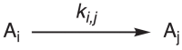
Natural photosynthesis is the only system for solar fuel production on a global scale and can serve as a blueprint for design of artificial photosynthesis. Oxygenic photosynthesis is initiated by the water-oxidation reaction catalyzed by the protein complex photosystem II (PSII) (Eq. 1).

(1)

An understanding of the water-oxidation reaction is crucial to the progress towards global solar fuel production in that this reaction provides abundant reducing equivalents for fuel production. However, despite decades of research, the mechanism of water oxidation in PSII is still unclear.

The catalytic center of PSII is the oxygen-evolving complex (OEC), located on the lumenal side of the membrane protein complex. The OEC is a Mn₄CaO₅ cluster with the geometry of a ‘distorted chair’.^1,2 It carries out the water-oxidation reaction (Eq. 1) in four light-driven one-electron steps. The intermediate oxidation states of the OEC are described by the S (storage) states;³ the most reduced state is S₀, whereas the most oxidized is S₄. The dark-stable state of the OEC is the S₁ state. Following light excitation and energy transfer in antenna cofactors, charge separation results in the OEC losing one electron, advancing it to the next S state. At the S₄ state, the OEC spontaneously releases dioxygen and resets its oxidation state to S₀. This S₄ to S₀ transition, when the most important chemistry happens, is very fast and light-independent, making it challenging to study the O-O bond-formation mechanism.

Substrate-water exchange experiments were developed to gain insight into substrate-water molecules, thereby probing the mechanism of the water-oxidation reaction.[4], [5], [6], [7], [8], [9] In such experiments, the OEC is advanced to either the S₀, S₁, S₂, or S₃ state by applying 3, 0, 1, or 2 flashes, respectively, to a dark-adapted PSII sample in an H₂¹⁶O-containing buffer. Then, a small amount of H₂¹⁸O is injected into the system followed by an incubation time t before giving one or more additional flashes to result in oxygen evolution. The yield of each isotopically labeled O₂ is detected by using membrane-inlet mass spectroscopy (MIMS). The single ¹⁸O-labeled O₂ yield, denoted as ³⁴Y for m/z = 34, and the double ¹⁸O-labeled O₂ yield, denoted as ³⁶Y, can be obtained simultaneously. The kinetics of substrate-water exchange in each of the intermediate S states can then be obtained by analyzing the relation between the yields, ³⁴Y and ³⁶Y, and the exchange time, t.

Previously, the data were analyzed by fitting the Y-versus-t plots using Eq. 2.[4], [5], [6], [7], [8], [9] The singly ¹⁸O-labeled O₂ yield, ³⁴Y, was fitted using two exponential terms, corresponding to the fast- and slow-exchange rate constants k_f and k_s, whereas the doubly ¹⁸O-labeled O₂ yield, ³⁶Y, was fitted with only one exponential term. The pre-exponential constant a describes the exponential component proportions of the fast and slow exchange in the ³⁴Y data and is derived from the ratio of [H₂¹⁸O] and [H₂¹⁶O] used in the experiments. The value of a has been very consistent in the literature, and the equation becomes ${}^{34}Y=1-0.57e^{-k_{f}t}-0.43e^{-k_{s}t}$. The reasoning is that the single ¹⁸O exchange requires exchange of either one or the other of the two substrate waters so the data were fit using a linear combination of two exponentials. On the other hand, the doubly ¹⁸O-labeled O₂ yield would be limited by the substrate water that exchanges more slowly. As a result, it was found that the value in Eq. 2 for k_s to fit ³⁴Y matches well with the value for k to fit ³⁶Y.

$${}^{34}Y=a\left(1-e^{-k_{f}t}\right)+\left(1-a\right)\left(1-e^{-k_{s}t}\right)$$

$${}^{36}Y=1-e^{-kt}$$ (2)

These results are important as they provide insight into the binding of the two substrate waters among all solvent water molecules near the OEC, thereby shedding light on the water-oxidation mechanism. It is, therefore, vital to ensure that the data interpretation is appropriate for a given model. The kinetic model to explain the data described above is based on an assumption of exponential terms, as shown in Eq. 2, but a detailed kinetic model is lacking. Here, we present two inclusive and generalized kinetic models with the derivations of their exact analytical solutions for analyzing and interpreting the experimental kinetic data. The first model has a single conformation and two substrate-water binding sites, applicable to most OEC systems. The other model has two interconvertible conformations with distinct substrate-water exchange kinetics, applicable to PSII samples in the S₂ state where the g = 2.0 and g = 4.1 conformations coexist.

The time-dependent concentrations of PSII that binds either two or one H₂¹⁸O can be calculated, and those concentrations translate directly to the time-dependent doubly- and singly-¹⁸O-labeled O₂ yields (Fig. 1). To construct the kinetic models, we start with a consideration of associative and dissociative exchange mechanisms at a single substrate-water binding site. Next, we expand the model to include two substrate-water binding sites to get our single-conformation model, and then we expand it again to include two conformations to get our double-conformation model.

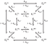
Fig. 1.

Scheme of the substrate-water exchange kinetic model at the OEC. The OCE has two substrate-water binding sites, shown as rectangles and ovals, each with corresponding different exchange rate constants. The ¹⁸O-labeled water and the resultant ¹⁸O-labeled O₂ are shown with gray background. Note that the concentrations of the labeled OECs at each time point translate directly to the labeled O₂ yields at those time points, as the two substrate waters would be used to produce dioxygen.

2. Materials and methods

Multiple-concentration rate equations are solved using the method below.¹⁰ Consider a system containing n components: A₁, A₂, …, A_j, …, A_n. Let the rate constant of conversion from any component A_i to another component A_j be k_i,j: (Note that k_i,i is defined to be 0.)

(3)

Then, the concentration change rate of the component A_j in the system is given by all conversions to A_j minus all conversions from A_j:

$$\frac{d\left[{\mathrm{A}}_{\mathrm{j}}\right]}{dt}=\sum _{i=1}^n\left(k_{i,j}\left[{\mathrm{A}}_{\mathrm{i}}\right]-k_{j,i}\left[{\mathrm{A}}_{\mathrm{j}}\right]\right)$$ (4)

All the rate equations in the system can be most conveniently expressed in a matrix form:

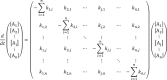(5)

Let c_t denote the vector containing the time-dependent concentrations [A₁], [A₂], ..., [A_n], and let k denote the n-by-n matrix containing the rate constants. Eq. 5 can thereby be expressed as follows:

$$\frac{d{\mathit{c}}_{\mathit{t}}}{dt}=\mathit{k}{\mathit{c}}_{\mathit{t}}$$ (6)

We can solve Eq. 6 to obtain c_t. The solution is given by

$${\mathit{c}}_{\mathit{t}}=e^{\mathit{k}t}{\mathit{c}}_0,$$ (7)

where c₀ is the concentration vector c_t at time 0. This solution is fully analogous to a differential equation that involves only real numbers. The definition of the matrix exponential that appears in Eq. 7 is again analogous to that of a real number exponential:

$$e^{\mathit{M}}=\sum _{i=0}^{\infty }\frac{1}{i!}{\mathit{M}}^i$$ (8)

The time-dependent concentration of the component A_j can be generalized to

$$\left[{\mathrm{A}}_{\mathrm{j}}\right]=\sum _{i=1}^n{c}_{j,i}{e}^{{\lambda }_{i}t},$$ (9)

where ${\lambda }_i$ are the eigenvalues of the n by n matrix k, and c_j,i are the constants corresponding to the component A_j and the eigenvalues ${\lambda }_i$. Because one of the eigenvalues is guaranteed to be 0, the solution is composed of a linear combination of n−1 exponential terms.

3. Results and discussion

3.1. Dissociative and associative mechanisms in a single-conformation, single-site model

In this section, we analyze the simplest building block of our kinetic model for substrate-water exchange. We show that no matter whether the system undergoes a dissociative or associative exchange mechanism, this model is equivalent to a simpler model without an intermediate.

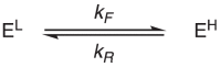
We first consider a dissociative water-exchange mechanism, where there is a rate-limiting substrate-water dissociation step, followed by a rapid association step (Eq. 10). Consider an enzyme with a single conformation and a single substrate-water binding site. An enzyme bound with a light water (H₂¹⁶O) is denoted by E^L, and that bound with a heavy water (H₂¹⁸O) by E^H. The intermediate enzyme with no water bound is denoted as E. We describe the first and second steps using the rate constants k' and k'', respectively.

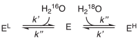(10)

Note that the dissociation rate constant k' is a first-order rate constant, whereas the association rate constant k'' is a second-order rate constant, because the latter involves both the enzyme and a water. The water concentrations are so high that they can be treated as constants; therefore, we can use the pseudo-first order rate constants k''[H₂¹⁶O] and k''[H₂¹⁸O] to describe the association step.

The rate equations of the system can be expressed in a matrix form, as described in Materials and Methods:

$$\frac{d}{dt}\left(\begin{array}{c}\left[{\mathrm{E}}^{\mathrm{L}}\right]\\ \left[\mathrm{E}\right]\\ \left[{\mathrm{E}}^{\mathrm{H}}\right]\end{array}\right)=\left(\begin{array}{ccc}-k^{\prime }& k^{″}\left[{\mathrm{H}}_2^{16}\mathrm{O}\right]& 0\\ k^{\prime }& -k^{″}\left[{\mathrm{H}}_2^{16}\mathrm{O}\right]-k^{″}\left[{\mathrm{H}}_2^{18}\mathrm{O}\right]& k^{\prime }\\ 0& k^{″}\left[{\mathrm{H}}_2^{18}\mathrm{O}\right]& -k^{\prime }\end{array}\right)\left(\begin{array}{c}\left[{\mathrm{E}}^{\mathrm{L}}\right]\\ \left[\mathrm{E}\right]\\ \left[{\mathrm{E}}^{\mathrm{H}}\right]\end{array}\right)$$ (11)

The solution is given by:

$$\left[{\mathrm{E}}^{\mathrm{L}}\right]=\frac{1}{\frac{k^{\prime }}{k^{″}\left[{\mathrm{H}}_2^{16}\mathrm{O}\right]}+\frac{1+r}{r}}\left[\frac{\left(k^{\prime }+k^{″}{c}_w\right)}{r{k}^{″}{c}_w}{e}^{-k^{\prime }t}+\frac{k^{\prime }}{k^{″}{c}_w}{e}^{-\left(k^{\prime }+k^{″}{c}_w\right)t}+1\right]$$

$$\approx \frac{r}{1+r}\left[\frac{1}{r}{e}^{-k^{\prime }t}+1\right]$$

$$\left[\mathrm{E}\right]=\frac{k^{\prime }}{k^{\prime }+k^{″}{c}_w}\left[-e^{-\left(k^{\prime }+k^{″}{c}_w\right)t}+1\right]$$

$$\approx 0$$

$$\left[{\mathrm{E}}^{\mathrm{H}}\right]=\frac{1}{\frac{k^{\prime }}{k^{″}\left[{\mathrm{H}}_2^{18}\mathrm{O}\right]}+\left(1+r\right)}\left[-\frac{k^{\prime }+k^{″}{c}_w}{k^{″}{c}_w}{e}^{-k^{\prime }t}+\frac{k^{\prime }}{k^{″}{c}_w}{e}^{-\left(k^{\prime }+k^{″}{c}_w\right)t}+1\right]$$

$$\approx \frac{1}{1+r}\left[-e^{-k^{\prime }t}+1\right]$$ (12)

We use c_w to denote the overall water concentration [H₂¹⁶O] + [H₂¹⁸O], and r to denote the ratio of the water concentrations [H₂¹⁶O]/[H₂¹⁸O]. The approximations are based on the assumption that the association rate is much faster than the dissociation rate (k'' ≫ k').

Next, we examine the associative exchange mechanism, where a rate-limiting substrate-water association is followed by a rapid dissociation (Eq. 13). The intermediate enzyme bound with two water molecules is denoted as E^LH. We still use k' to describe the first, slow step and k'' the second, fast step, so in this case, k' is the association rate constant. Again, the pseudo-first order association rate constants are k'[H₂¹⁸O] and k'[H₂¹⁶O].

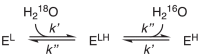(13)

Similarly, we can solve the rate equations using the same method. The solution is more complicated and can be found in the Appendix. Here, for simplicity, we only show the solution after the approximation that k'' ≫ k'.

$$\left[{\mathrm{E}}^{\mathrm{L}}\right]\approx \frac{r}{1+r}\left[\frac{1}{r}{e}^{-\frac{1}{2}{k}^{\prime }{c}_{w}t}+1\right]$$

$$\left[{\mathrm{E}}^{\text{LH}}\right]\approx 0$$

$$\left[{\mathrm{E}}^{\mathrm{H}}\right]\approx \frac{1}{1+r}\left[-e^{-\frac{1}{2}{k}^{\prime }{c}_{w}t}+1\right]$$ (14)

Since the concentrations of the intermediates in both models (E and E^LH) are both 0 under the limit of k'' ≫ k', we can simplify the model to one without an intermediate:

, (15)

where k_F is the apparent first-order forward rate constant and k_R is the apparent first-order reverse rate constant. The time-dependent concentrations of E^L and E^H in this simplified model are given by:

$$\left[{\mathrm{E}}^{\mathrm{L}}\right]=\frac{k_R}{k_F+k_R}\left[\frac{k_F}{k_R}{e}^{-\left(k_F+k_R\right)t}+1\right]=\frac{k_R}{k_F+k_R}\left[\frac{k_F}{k_R}{e}^{-k^{*}t}+1\right]$$

$$\left[{\mathrm{E}}^{\mathrm{H}}\right]=\frac{k_F}{k_F+k_R}\left[-e^{-\left(k_F+k_R\right)t}+1\right]=\frac{k_F}{k_F+k_R}\left[-e^{-k^{*}t}+1\right]$$ (16)

$k^{*}$ denotes the overall decay constant in the exponential term, which equals k_F + k_R.

In the final step in the analysis, we compare the dissociative (Eq. 10) and associative (Eq. 13) models with the simplified one (Eq. 15) by equating the coefficients between Eqs. 12, 14 and Eq. 16. From the pre-exponential terms, we get

$$r\equiv \frac{\left[{\mathrm{H}}_2^{16}\mathrm{O}\right]}{\left[{\mathrm{H}}_2^{18}\mathrm{O}\right]}=\frac{k_R}{k_F},$$ (17)

and from the exponent, we have

$$k^{*}\equiv k_F+k_R=C_m{k}^{\prime },$$ (18)

where k' is the rate constant for the rate-limiting dissociation step in Eq. 10, or that for the rate-limiting association step in Eq. 13, and C_m is the mechanism-dependent constant: C_m = 1 for the dissociative mechanism and C_m = c_w/2 for the associative mechanism. This makes sense from a dimensional analysis perspective. k* is a first-order rate constant with a unit of s⁻¹, and so is the dissociative rate constant k'; thus, the dissociative C_m is dimensionless. On the other hand, the associative rate constant k' is a second-order rate constant with a unit of s⁻¹M⁻¹, so the associative C_m has a unit of M. This mechanism-dependent constant can potentially help to distinguish between the two exchange mechanisms and shed light on the geometry and oxidation state of the Mn ion involved in substrate-water binding, as will be discussed further in section 3.8.

Looking at the solution of the simplified model in Eq. 16, the information about the equilibrium, which is dictated by the light and heavy water concentrations, can be found in the ratio of the reverse and forward rate constants k_R/k_F Eq. 17; the information about the rate of the first slow step, k', can be found in the sum of the forward and reverse rate constants k_F + k_R (Eq. 18); and the information about the second fast step k'' is lost, because it doesn't have an impact on the apparent rate.

With the relation in Eq. 17, we then substitute the forward rate constant with k, and reverse rate constant with r∙k, so Eq. 15 becomes:

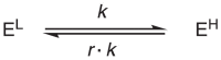(19)

Plugging (15), (17) into Eq. 14, we get:

$$\left[{\mathrm{E}}^{\mathrm{L}}\right]=\frac{r}{1+r}\left[\frac{1}{r}{e}^{-C_m{k}^{\prime }t}+1\right]$$

$$\left[{\mathrm{E}}^{\mathrm{H}}\right]=\frac{1}{1+r}\left[-e^{-C_m{k}^{\prime }t}+1\right]$$ (20)

3.2. Single-conformation model with two binding sites

In this section, we consider the single-conformation model with two substrate-water binding sites, shown in Eq. 21 for a dissociative system, and in Eq. 22 for an associative system.

(21)

(22)

Experimentally, it is observed that the exchange at one of the binding sites is fast, where the rate constants associated are k_f' and k_f'', and that the exchange at the other site is slow, described by the rate constants k_s' and k_s''. E^LL denotes an OEC that binds two light waters, E^LH denotes an OEC that binds one light water and one heavy water, and so on. The two exchange reactions can occur independently in any order and result in an equilibrium.

We have shown in Section 3.1 that the concentrations of the intermediates are approximately zero given that k'' ≫ k'; therefore, we can omit the intermediates and simplify the chemical equations. Both Eqs. 21-22 can be simplified from 8 components to 4, as shown in Eq. 23, which is the same model as depicted in Fig. 1. We call Eq. 23 the single-conformation model. This model is suitable for analyzing the majority of previously-reported substrate-water exchange data,^5,7,8 in which only a single OEC conformation was involved.

(23)

The rate equations arranged in matrix form are given by:

$$\frac{d}{dt}\left(\begin{array}{c}\left[{\mathrm{E}}^{\text{LL}}\right]\\ \left[{\mathrm{E}}^{\text{LH}}\right]\\ \left[{\mathrm{E}}^{\text{HL}}\right]\\ \left[{\mathrm{E}}^{\text{HH}}\right]\end{array}\right)=\left(\begin{array}{cccc}-k_f-k_s& r{k}_f& r{k}_s& 0\\ k_f& -r{k}_f-k_s& 0& r{k}_s\\ k_s& 0& -k_f-r{k}_s& r{k}_f\\ 0& k_s& k_f& -r{k}_f-r{k}_s\end{array}\right)\left(\begin{array}{c}\left[{\mathrm{E}}^{\text{LL}}\right]\\ \left[{\mathrm{E}}^{\text{LH}}\right]\\ \left[{\mathrm{E}}^{\text{HL}}\right]\\ \left[{\mathrm{E}}^{\text{HH}}\right]\end{array}\right)$$ (24)

The individual concentrations [E^LL], [E^LH], [E^HL], and [E^HH] can be solved as described in section 3.1. The observables in the substrate-water exchange experiments, singly-labeled O₂ yield, ³⁴Y, and doubly-labeled O₂ yield, ³⁶Y, can be expressed in terms of the labeled OEC concentrations, [E^LH], [E^HL], and [E^HH]:

$${}^{34}Y\propto \left[{\mathrm{E}}^{\text{LH}}\right]+\left[{\mathrm{E}}^{\text{HL}}\right]=\frac{2r}{{(1+r)}^2}\left[-\frac{1}{r}{e}^{{\lambda }_{1}t}-\frac{r-1}{2r}{e}^{{\lambda }_{2}t}-\frac{r-1}{2r}{e}^{{\lambda }_{3}t}+1\right]$$

$${}^{36}Y\propto \left[{\mathrm{E}}^{\text{HH}}\right]=\frac{1}{{(1+r)}^2}\left[e^{{\lambda }_{1}t}-e^{{\lambda }_{2}t}-e^{{\lambda }_{3}t}+1\right]$$ (25)

The λ's are the eigenvalues of the k matrix in Eq. 24 and are given by

$${\lambda }_1=-C_m\left(k_f^{\prime }+k_s^{\prime }\right)=-\left(k_f^{*}+k_s^{*}\right)$$

$${\lambda }_2=-C_m{k}_f^{\prime }=-k_f^{*}$$

$${\lambda }_3=-C_m{k}_s^{\prime }=-k_s^{*}$$

$${\lambda }_4=0,$$ (26)

where C_m = 1 for a dissociative mechanism and C_m = c_w/2 for an associative mechanism, and k_f' and k_s' are the rate constants of the dissociation steps in Eq. 21 or those of the association steps in Eq. 22. For simplicity, we substitute C_mk' with k* as shown in Eq. 18. The eigenvalues reflect the substrate-water exchange rate of the fast-exchanging site (λ₂), that of the slowly-exchanging site (λ₃), and the two combined (λ₁). When k_f' ≫ k_s', we have λ₁ ≈ λ₂ = −k_f*, so Eq. 25 becomes:

$${}^{34}Y\propto \left[-\frac{r+1}{2r}{e}^{-k_f^{*}t}-\frac{r-1}{2r}{e}^{-k_s^{*}t}+1\right]$$

$${}^{36}Y\propto \left[-e^{-k_s^{*}t}+1\right]$$ (27)

This is the same expression as Eq. 2, which was used to fit the data from substrate-water exchange experiments, with r = 6.4, the [H₂¹⁶O]/[H₂¹⁸O] used in the experiments.^5,7,8

Eq. 2 is a good approximation of the analytical solution of the single-conformation model (Eq. 25) in the limit when k_f' ≫ k_s' and appears to work pretty well to describe the experimental data.^5,7,8 However, for other regimes, the Y-versus-t relation deviates from what is described by Eq. 27. If equal amounts of H₂¹⁶O and H₂¹⁸O are used in the substrate-water exchange experiments, such that r = 1, we have the pre-exponential terms (r−1)/2r = 0 in Eq. 25, and only one exponential term would remain in ³⁴Y: ³⁴Y ∝ {1 − exp[−(k_f*+k_s*)t]}. On the other hand, if k_f' ≫ k_s' does not hold true, ³⁴Y would show a third exponential term with λ₁ as the decay constant, which reflects both k_f' and k_s'. Thus, when using Eq. 2 to fit experimental substrate-water exchange data, it is important to make sure that the experiments are performed under conditions where k_f' ≫ k_s' and r ≠ 1.

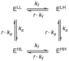
3.3. Double-conformation model

Finally, we expand the single-conformation model in Section 3.2 to include a second conformation. The two conformations (E₁ and E₂) may have different sets of substrate-water exchange rates (k_f,1, k_s,1, and k_f,2, k_s,2, respectively) and are connected by conformation-change rate constants k_c,1 and k_c,2. (Eq. 28) We call Eq. 28 the double-conformation model. This model is suitable for analyzing the substrate-water exchange data of a system where the S₂ g = 2.0 and S₂ g = 4.1 conformations coexist.¹¹

(28)

Again, the yields ³⁴Y and ³⁶Y can be expressed in terms of the concentrations of the singly- and doubly-labeled enzymes, respectively. The expression is more complex and involves many parameters. Here, we will present the complete expression of the solution and the definitions of the parameters before diving into further discussion. The yields are given by

$$\begin{array}{ccc}& & {}^{34}Y\propto \left[{\mathrm{E}}_1^{\text{LH}}\right]+\left[{\mathrm{E}}_1^{\text{HL}}\right]+\left[{\mathrm{E}}_2^{\text{LH}}\right]+\left[{\mathrm{E}}_2^{\text{HL}}\right]=\frac{2r}{{(1+r)}^2}[-\frac{1}{r}\left(c_1^{+}{e}^{{\lambda }_1^{+}t}+c_1^{-}{e}^{{\lambda }_1^{-}t}\right)\hfill \\ & & -\frac{r-1}{2r}\left(c_2^{+}{e}^{{\lambda }_2^{+}t}+c_2^{-}{e}^{{\lambda }_2^{-}t}\right)-\frac{r-1}{2r}\left(c_3^{+}{e}^{{\lambda }_3^{+}t}+c_3^{-}{e}^{{\lambda }_3^{-}t}\right)+1]\hfill \end{array}$$

$$\begin{array}{ccc}& & {}^{36}Y\propto \left[{\mathrm{E}}_1^{\text{HH}}\right]+\left[{\mathrm{E}}_2^{\text{HH}}\right]=\frac{1}{{(1+r)}^2}[\left(c_1^{+}{e}^{{\lambda }_1^{+}t}+c_1^{-}{e}^{{\lambda }_1^{-}t}\right)-\left(c_2^{+}{e}^{{\lambda }_2^{+}t}+c_2^{-}{e}^{{\lambda }_2^{-}t}\right)\hfill \\ & & -\left(c_3^{+}{e}^{{\lambda }_3^{+}t}+c_3^{-}{e}^{{\lambda }_3^{-}t}\right)+1],\hfill \end{array}$$ (29)

where the $\lambda$'s in the exponential terms are the eigenvalues of the k matrix describing this model, given by

$$\begin{array}{ccc}& & {\lambda }_1^{+,-}=\frac{1}{2}[-\left(k_{f,1}^{*}+k_{s,1}^{*}+k_{f,2}^{*}+k_{s,2}^{*}+k_{c,1}+k_{c,2}\right)\hfill \\ & & \pm \sqrt{{\left(k_{f,1}^{*}+k_{s,1}^{*}+k_{f,2}^{*}+k_{s,2}^{*}+k_{c,1}+k_{c,2}\right)}^2-4\left[\right(k_{f,1}^{*}+k_{s,1}^{*}\left)\right(k_{f,2}^{*}+k_{s,2}^{*})+(k_{f,1}^{*}+k_{s,1}^{*})k_{c,1}+(k_{f,2}^{*}+k_{s,2}^{*})k_{c,2}]}]\hfill \end{array}$$

$$\begin{array}{ccc}& & {\lambda }_2^{+,-}=\frac{1}{2}[-\left(k_{f,1}^{*}+k_{f,2}^{*}+k_{c,1}+k_{c,2}\right)\hfill \\ & & \pm \sqrt{{\left(k_{f,1}^{*}+k_{f,2}^{*}+k_{c,1}+k_{c,2}\right)}^2-4\left(k_{f,1}^{*}{k}_{s,2}^{*}+k_{f,1}^{*}{k}_{c,1}+k_{f,2}^{*}{k}_{c,2}\right)}]\hfill \end{array}$$

$$\begin{array}{ccc}& & {\lambda }_3^{+,-}=\frac{1}{2}[-\left(k_{s,1}^{*}+k_{s,2}^{*}+k_{c,1}+k_{c,2}\right)\hfill \\ & & \pm \sqrt{{\left(k_{s,1}^{*}+k_{s,2}^{*}+k_{c,1}+k_{c,2}\right)}^2-4\left(k_{s,1}^{*}{k}_{s,2}^{*}+k_{s,1}^{*}{k}_{c,1}+k_{s,2}^{*}{k}_{c,2}\right)}]\hfill \end{array}$$

$${\lambda }_4=-\left(k_{c,1}+k_{c,2}\right)$$

$${\lambda }_5=0.,$$ (30)

where k* C_m ∙ k' = (1+r) ∙ k; and the pre-exponential constants in Eq. 29 are given by

$$c_i^{+,-}=\frac{1}{2}\pm \frac{1}{2}\left\{\frac{k_{c,1}+k_{c,2}}{\Delta {\lambda }_i^{+-}}+\frac{\left(k_{c,1}-k_{c,2}\right)\left[x\left(-k_{f,1}^{*}+k_{f,2}^{*}\right)+y\left(-k_{s,1}^{*}+k_{s,2}^{*}\right)\right]}{\left(k_{c,1}+k_{c,2}\right)\Delta {\lambda }_i^{+-}}\right\},$$ (31)

where $[\begin{array}{c}x=1,y=1ifi=1\\ x=1,y=0ifi=2\\ x=0,y=1ifi=3\end{array}$and ∆λ_i⁺⁻ is defined as λ_i⁺ − λ_i⁻. Note that, for example, λ₁^+,− are two eigenvalues, and λ₁⁺ corresponds to the + sign of the ± in the expression, whereas λ₁⁻ corresponds to the − sign. The interpretation is the same for c_i^+,−.

We found that the solution of the single-conformation model (Eqs. 25–26) is analogous to that of the double-conformation model (Eqs. 29–31). Each of the eigenvalues λ_1-3 in the single-conformation model (Eq. 26) splits into two eigenvalues, λ_1-3⁺ and λ_1-3⁻, in the double-conformation model (Eq. 30). Similar to λ_1-3 in Eq. 26, the eigenvalues in Eq. 30 reflect the substrate-water exchange rates of the fast-exchanging sites in both conformations (λ₂^+,−), those of the slowly-exchanging sites (λ₃^+,−), and those of the all four sites (λ₁^+,−). The conformational change rates, k_c,1 and k_c,2, are found in all the non-zero eigenvalues, including λ₄, which is −(k_c,1 + k_c,2), although this eigenvalue does not appear in the expression of the concentrations in Eq. 29. Finally, each exponential term, exp(λ_it), in Eq. 25, also splits into a linear combination of two exponentials, [c_i⁺ exp(λ_i⁺t) + c_i⁻ exp(λ_i⁻t)], in Eq. 29. As a result, in the double-conformation model, both ³⁴Y and ³⁶Y are composed of a linear combination of 6 exponentials.

The pre-exponential constants c_i^+,− precede the exponential terms containing the eigenvalues λ_i^+,−. As mentioned before, each λ reflects a different subset of the substrate-water exchange rate constants, and so does each c. Therefore, we see in Eq. 31 that c₂^+,− consists of the fast-exchanging rate constants in both conformations, c₃^+,− consists of the slowly-exchanging rate constants, and c₁^+,− consists of all four rate constants.

The complete analytical solution of the double-conformation model (Eqs. 29-31) is so complex that one cannot easily see the physical meanings as it is. Thus, only for the purpose of getting a better grasp of the physical meanings, we apply some approximations to simplify the expressions, although as discussed later in Section 3.5, some approximations we apply here might not be valid when dealing with the experimental data.

We first assume that the conformational change is much slower than the substrate-water exchange (k_c ≪ k_f* & k_s*). This way, the square root terms in Eq. 30, ∆λ_i⁺⁻ λ_i⁺ − λ_i⁻, can be simplified to:

$$\Delta {\lambda }_i^{+-}\approx \left|x\left(k_{f,1}^{*}-k_{f,2}^{*}\right)+y\left(k_{s,1}^{*}-k_{s,2}^{*}\right)\right|,$$ (32)

where $[\begin{array}{c}x=1,y=1ifi=1\\ x=1,y=0ifi=2\\ x=0,y=1ifi=3\end{array}$

Thereby, we obtain expressions of λ_1-3^+,−, now without the conformational change rate constants k_c,1 and k_c,2. λ_1-3^+,− becomes:

$${\lambda }_1^{+,-}\approx \frac{1}{2}\left[-\left(k_{f,1}^{*}+k_{s,1}^{*}+k_{f,2}^{*}+k_{s,2}^{*}\right)\pm \left|k_{f,1}^{*}+k_{s,1}^{*}-k_{f,2}^{*}-k_{s,2}^{*}\right|\right]$$

$${\lambda }_2^{+,-}\approx \frac{1}{2}\left[-\left(k_{f,1}^{*}+k_{f,2}^{*}\right)\pm \left|k_{f,1}^{*}-k_{f,2}^{*}\right|\right]$$

$${\lambda }_3^{+,-}\approx \frac{1}{2}\left[-\left(k_{s,1}^{*}+k_{s,2}^{*}\right)\pm \left|k_{s,1}^{*}-k_{s,2}^{*}\right|\right]$$ (33)

To further simplify the expressions containing absolute values, we conveniently assume that both sites in conformation 1 exchange faster than those in conformation 2 (i.e. k_f,1* > k_f,2* & k_s,1* > k_s,2*). Note that whatever assumption made here to remove the absolute value leads to the same result. After the simplification, the eigenvalues can be given by:

$${\lambda }_1^{+}\approx -\left(k_{f,2}^{*}+k_{s,2}^{*}\right)$$

$${\lambda }_1^{-}\approx -\left(k_{f,1}^{*}+k_{s,1}^{*}\right)$$

$${\lambda }_2^{+}\approx -k_{f,2}^{*}$$

$${\lambda }_2^{-}\approx -k_{f,1}^{*}$$

$${\lambda }_3^{+}\approx -k_{s,2}^{*}$$

$${\lambda }_3^{-}\approx -k_{s,1}^{*}$$ (34)

We see that the λ_i⁺ and λ_i⁻ now reflect the substrate-water exchange kinetics of the individual conformation. λ_i⁺ corresponds to the slow conformation (conformation 2 in this case, corresponding to k_f,2* and k_s,2*), whereas λ_i⁺ corresponds to the fast conformation (conformation 1, corresponding to k_f,1* and k_s,1*).

With k_c ≪ k_f* & k_s*, Eq. 32, and k_f,1* > k_f,2* & k_s,1* > k_s,2*, we now simplify the pre-exponential constants in Eq. 31:

$$\begin{array}{ccc}& & c_i^{+,-}\approx \frac{1}{2}\pm \frac{1}{2}\left\{\frac{\left(k_{c,1}-k_{c,2}\right)\left[x\left(-k_{f,1}^{*}+k_{f,2}^{*}\right)+y\left(-k_{s,1}^{*}+k_{s,2}^{*}\right)\right]}{\left(k_{c,1}+k_{c,2}\right)\left|x\left(k_{f,1}^{*}-k_{f,2}^{*}\right)+y\left(k_{s,1}^{*}-k_{s,2}^{*}\right)\right|}\right\}\hfill \\ & & \approx \frac{1}{2}\left[1\mp \frac{k_{c,1}-k_{c,2}}{k_{c,1}+k_{c,2}}\right]\hfill \end{array}$$ (35)

Note that c_i⁺ corresponds to the + in the ± and the − in the ∓. Now, we have expressions for c_i⁺ and c_i⁻ that are not i-dependent:

$$[\begin{array}{c}{c}_i^{+}\approx \frac{k_{c,2}}{k_{c,1}+k_{c,2}}\\ c_i^{-}\approx \frac{k_{c,1}}{k_{c,1}+k_{c,2}}\end{array}$$ (36)

c_i⁺ is the equilibrium fraction of the slow conformation, whereas c_i⁻ is that of the fast one. We will drop the subscript i in the rest of this section.

With some rearrangements, the yields of labeled O₂ in Eq. 29 become:

$$\begin{array}{ccc}& & {}^{34}Y\propto c^{+}\left[-\frac{1}{r}·e^{{\lambda }_1^{+}t}-\frac{r-1}{2r}·e^{{\lambda }_2^{+}t}-\frac{r-1}{2r}·e^{{\lambda }_3^{+}t}+1\right]\hfill \\ & & +c^{-}\left[-\frac{1}{r}·e^{{\lambda }_1^{-}t}-\frac{r-1}{2r}·e^{{\lambda }_2^{-}t}-\frac{r-1}{2r}·e^{{\lambda }_3^{-}t}+1\right]\hfill \end{array}$$

$${}^{36}Y=c^{+}\left[e^{{\lambda }_1^{+}t}-e^{{\lambda }_2^{+}t}-e^{{\lambda }_3^{+}t}+1\right]+c^{-}\left[e^{{\lambda }_1^{-}t}-e^{{\lambda }_2^{-}t}-e^{{\lambda }_3^{-}t}+1\right]$$ (37)

If we further assume k_f* ≫ k_s*, we have ${\lambda }_1$≈${\lambda }_2$ and

$$\begin{array}{ccc}& & {}^{34}Y\propto c^{-}\left[-\frac{r+1}{2r}{e}^{-k_{f,1}^{*}t}-\frac{r-1}{2r}{e}^{-k_{s,1}^{*}t}+1\right]\hfill \\ & & +c^{+}\left[-\frac{r+1}{2r}{e}^{-k_{f,2}^{*}t}-\frac{r-1}{2r}{e}^{-k_{s,2}^{*}t}+1\right]\hfill \end{array}$$

$${}^{36}Y\propto c^{-}\left[-e^{-k_{s,1}^{*}t}+1\right]+c^{+}\left[-e^{-k_{s,2}^{*}t}+1\right]$$ (38)

We can see clearly that Eq. 38 is a linear combination of the single-conformation model solution (Eq. 27) based on the equilibrium fractions of the two conformations (c⁺ and c⁻). When k_c ≪ k_f* & k_s* is true, the system described by the double-conformation model acts as if the two conformations carry out the substrate-water exchange reaction independently. However, when the above assumptions are not true, the complete, unsimplified model is needed to describe the system accurately.

3.4. Application of the single-conformation model to published data

Previously, experimental substrate-water exchange data were reported on Ca²⁺-containing PSII⁸ and Sr²⁺-containing PSII⁷ from spinach for each of the S_i (i = 0 – 3) states, and the data were all analyzed using linear combinations of exponential terms (Eq. 2). In addition, substrate-water exchange data using Ca²⁺-containing cyanobacterial PSII in the S₂ and S₃ states were also reported.¹¹ As we pointed out in section 3.2, Eq. 2 is a very good approximation of the complete analytical solution of the single-conformation model shown in Eq. 25 when k_f' ≫ k_s' is satisfied. Therefore, we expect to obtain similar results when fitting the data using the single-conformation model compared with the exponential fittings using Eq. 2.

Here, we demonstrate the fit of the S₂ state data of Ca²⁺-containing PSII and Sr²⁺-containing PSII^7,8,11 using the single-conformation model (Eq. 25) and using linear combinations of exponentials (Eq. 2) (Table 1). We get very similar results except for the k_f of Sr²⁺-containing PSII, which was too fast to be fully resolved by MIMS.⁷ The resolution was capped at 120 s⁻¹ by the time needed to allow injection and mixing of ¹⁸O-labeled H₂O. Although the single-conformation model suggests a very fast k_f for Sr²⁺-containing PSII based on the data, the model fits the data similarly well as long as k_f is larger than 120 s⁻¹.

Table 1.

Summary of the rate constants obtained from the substrate-water exchange experiments^7,8,11 using the single-conformation model (Eq. 25) described in this work and using linear combinations of exponentials (Eq. 2), which was originally used in Refs. 7, 8, 11 to fit the data. k_f* and k_s* denote the apparent fast- and slowly-exchanging rate constants, whose relation to the elementary associative or dissociative rate constant k' is described by k* = C_m ∙ k' and depends on the exchange mechanism.

Sample	Model	kf* (s−1)	ks* (s−1)
Ca2+-PSII (cyanobacterium)11	This work (Eq. 25)	94	1.1
	Ref. 11 (Eq. 2)	102	1.1
Ca2+-PSII (spinach)8	This work (Eq. 25)	120	2.0
	Ref. 8 (Eq. 2)	120	2.0
Sr2+-PSII (spinach)7	This work (Eq. 25)	5700	8.3
	Ref. 7 (Eq. 2)	>120	9.0

3.5. Application of the double-conformation model to published data

It was revealed by EPR spectroscopy that there are two conformations of the S₂ state, one with an EPR signal centered at g = 2.0[12], [13], [14], [15], [16], [17], [18] and the other at g = 4.1.^15,[19], [20], [21], [22] The modeled S₂-state structures are depicted in Fig. 2. The g = 2.0 conformation corresponds to a Mn oxidation-state pattern of (III, IV, IV, IV from Mn1 to Mn4) and an open-cubane structure. Here, we follow the nomenclature used in references (11,23) and denote the low-spin structure by S₂^A, where the A indicates an open-cubane configuration. On the other hand, the structure of the g = 4.1 conformation is under debate, partly due to the absence of crystal structures. There are currently three models that may account for the g = 4.1 EPR signal. It was first proposed that the g = 4.1 conformation corresponds to a closed-cubane structure, where the O5 µ-oxo ligand moves away from the dangling Mn4 and towards Mn1, with an oxidation-state swap between Mn1 and Mn4, resulting in an oxidation-state pattern of (IV, IV, IV, III).[24], [25], [26] This structure is denoted by S₂^B, where the B indicates a closed cubane configuration. Recently, two alternative structures were proposed, both with open-cubane-like structures. One has an additional hydroxide bound on Mn1 and with an oxidation-state pattern of (IV, IV, IV, III), the same as the closed-cubane structure[27], [28], [29] and is denoted by S₂^AW, where the A indicates an open-cubane structure and the W indicates an additional water ligand. The other has O4 protonated, with an oxidation-state pattern of (III, IV, IV, IV)³⁰ and is denoted by S₂^PI, meaning proton isomer. No matter what structure the g = 4.1 conformation corresponds to, it is likely that the two conformations exhibit distinct substrate-water exchange kinetics. The S₂^BW conformation is similar to S₂^B, with an additional water bound on Mn4. It was proposed that the conformational change between S₂^A and S₂^B might go through S₂^A, S₂^AW,S₂^BW, and finally to S₂^B,^11,23 which we discuss in more detail in Section 3.7.

Fig. 2.

Structural models of the S₂ state of the OEC. S₂^A is the open-cubane structure corresponding to the multiline g = 2 EPR signal. For the g = 4.1 EPR signal, various models have been proposed, including S₂^B, S₂^AW, and S₂^PI. The additional water ligands in S₂^AW and S₂^BW are highlighted with red glows. Note that in S₂^A and S₂^PI, the oxidation state pattern of the Mn ions is (III, IV, IV, IV) for Mn1 to Mn4, whereas in S₂^B, S₂^AW, and S₂^BW, the pattern is (IV, IV, IV, III).

Recently, substrate-water exchange data for samples prepared with varied proportions of the two S₂ state conformations were reported.¹¹ In untreated cyanobacterial PSII, only the S₂ state g = 2.0 conformation is observed.^11,31 de Lichtenberg and Messinger raised the pH to increase the proportion of the S₂ state g = 4.1 conformation, and carried out the substrate-water exchange experiments.¹¹ The system with coexisting conformations can be suitably described by our double-conformation model (Eq. 28). As discussed in Section 3.3, even in a simplified scenario where the rate of conformation change is much slower than the rates of the substrate-water exchange (k_c ≪ k_f* & k_s*), the data would reflect a condition where the two conformations carry out the substrate-water exchange reactions independently, so it is expected that the data would be harder to interpret, as there are more variables to fit. de Lichtenberg and Messinger fit their data using the following equations:¹¹

$${}^{34}Y=a\left(1-e^{-k_{f}t}\right)+\left(1-a\right)\left[b\left(1-e^{-k_{i}t}\right)+\left(1-b\right)\left(1-e^{-k_{s}t}\right)\right]$$

$${}^{36}Y=b\left(1-e^{-k_{i}t}\right)+\left(1-b\right)\left(1-e^{-k_{s}t}\right),$$ (39)

where the pre-exponential constant a describes the exponential component proportions of the fast and slow exchange in the ³⁴Y data and is related to the labeled-water ratio r, and b represents the equilibrium ratio of the two conformations, which corresponds to c⁺ and c⁻ of our model in Section 3.3. In Eq. 39, only three rate constants are fitted; in addition to the fast and slow rate constants, k_f and k_s, an intermediate rate constant, k_i, is added to the linear combinations of exponentials. Due to the complex nature of the data, it was not clear how to assign k_s. It was proposed to be either the slowly-exchanging rate constant in S₂ state g = 2.0 conformation, or the conformational change rate constant. On the other hand, k_i was assigned to be the slowly-exchanging rate constant of the S₂ state g = 4.1 conformation.¹¹ Here, with our double-conformation model in hand, we were able to assign k_s, as well as other rate constants in Eq. 39 explicitly to the rate constants of the double-conformation kinetic model (Eq. 28). We were also able to gain insights in identifying the regime where Eq. 39 is valid to fit the data.

We can rearrange Eq. 39 to Eq. 40:

$$\begin{array}{ccc}& & {}^{34}Y=\left(1-b\right)\left[a\left(1-e^{-k_{f}t}\right)+\left(1-a\right)\left(1-e^{-k_{s}t}\right)\right]\hfill \\ & & +b\left[a\left(1-e^{-k_{f}t}\right)+\left(1-a\right)\left(1-e^{-k_{i}t}\right)\right]\hfill \end{array}$$

$${}^{36}Y=\left(1-b\right)\left(1-e^{-k_{s}t}\right)+b\left(1-e^{-k_{i}t}\right)$$ (40)

We can see that Eq. 40 is a further simplification of Eq. 38, which is an already-simplified version of the complete analytical solution of the double-conformation model, with the additional assumption of the two conformations sharing the fast exchange rate (k_f,1* = k_f,2*). In summary, it takes three assumptions to simplify the complete solution to Eq. 40. The assumptions are: (a) the rate of conformational change is much slower than that of water exchange (k_c ≪ k_f* & k_s*); (b) the rate at the fast-exchanging site is much faster than that at the slow one (k_f' ≫ k_s'); and (c) the fast-exchanging rate is the same for the two conformations (k_f,1* = k_f,2*). By comparing Eq. 40 to Eq. 38, we were able to assign the k's in Eq. 40 to the k's in the double-conformation model shown in Eq. 29. k_f in Eq. 40 is assigned to k_f,1* and k_f,2* in Eq. 29, k_i to k_s,2*, and k_s to k_s,1*. The assignments confirm that k_s corresponds to the slowly-exchanging rate constant of conformation 1 (k_s,1*), rather than the conformational change rate constants (k_c,1 or k_c,2). This makes sense because the contribution of k_c,1 and k_c,2 in the exponents disappear after making the approximation that k_c ≪ k_f* & k_s* (Eq. 30 to Eq. 34), so there is no contribution from the conformational change rate to the apparent rate constants of substrate-water exchange under this assumption. Without the assumption of k_c ≪ k_f* & k_s*, the solution cannot be reduced to a simple form as shown in Eq. 39. Therefore, we conclude that k_s in Eq. 39 is not the conformational change rate constants (k_c,1 or k_c,2). Note that in our double-conformation model, the relation between the apparent rate constant k*, the elementary associative or dissociative rate constant k', and the compound associative or dissociative rate constant k is k* = C_m ∙ k' = (1+r) ∙ k. The assumption that k_f' ≫ k_s' in (b) is most appropriate in the context of the derivation, but saying k_f' ≫ k_s' is the same as saying k_f* ≫ k_s* or k_f≫ k_s, because the differences between the three are just scaling factors.

We can proceed with the analysis using the complete analytical solution of the double-conformation model (Eq. 29) without making those three assumptions above. After obtaining the rate constants using this model, we will come back to examine if Eq. 39 is valid for the specific data set. Both the ³⁴Y and ³⁶Y data were fitted simultaneously, rather than separately, to find a single set of parameters that minimized the sum of fitting errors from both yields. We tried fitting the data with 6 variables (k_f,1*, k_s,1*, k_f,2*, k_s,2*, k_c,1, and k_c,2), but the results were unsatisfactory due to too few restraints. Therefore, we assumed that k_f,1* and k_s,1* can be treated as known parameters to reduce the number of variables. Here, we let conformation 1, described by k_f,1* and k_s,1*, be the S₂ state g = 2.0 conformation, and conformation 2, described by k_f,2* and k_s,2*, be the S₂ state g = 4.1 conformation. Because the S₂ state g = 2.0 conformation is the predominant one of the two, its water-exchange kinetics have already been well-studied.^7,8,11 We pre-set k_f,1* and k_s,1* in the double-conformation model based on the analysis in Section 3.4 on the single-conformation experiments (Table 1). After restraining these two parameters, the reliability of the fit using Eq. 29 was dramatically improved.

The double-conformation experiments were done using PSII core complexes from the cyanobacterium Thermosynechococcus elongatus, and ideally, we would use the k_f,1* and k_s,1* values from the same organism. The k_f,1* and k_s,1* values for Ca²⁺-containing PSII were taken from the single-conformation results using the same organism.¹¹ However, single-conformation data were not available for Sr²⁺-containing PSII in the cyanobacterium T. elongatus because the Sr²⁺ substitution appeared to promote the S₂ state g = 4.1 conformation significantly, already making the second conformation detectable.¹¹ We, therefore, used the data taken from spinach PSII membranes.⁷ Although it is possible that the PSII in these two organisms exhibit distinct substrate-water exchange kinetics, it should be reasonable to assume that they are very similar based on the highly conserved amino-acid residues near the OEC.³² We also assumed that the change of pH from 6 to 8 does not significantly affect the substrate-water exchange kinetics in conformation 1; we also note that there is a lack of a pH dependence for the S₁- to S₂-state transition.^9,33

With k_f,1* and k_s,1* fixed, we analyzed the experimental substrate-water exchange data performed in a double-conformation system in the S₂ state¹¹ using our double-conformation model (Eq. 29). The analyses were run using MATLAB scripts. We looked at three conditions where the secondary S₂ state g = 4.1 conformation is present. One is done using Ca²⁺-containing PSII at pH 8.6, and the other two using Sr²⁺-containing PSII at pH 6.0 and pH 8.3. The results of the fitting can be found in Fig. 3 and Table 2.

Fig. 3.

Substrate-water exchange data in two-conformation systems taken from reference 11 and fitted using the double-conformation model (Eq. 29). The singly-¹⁸O-labeled O₂ yield, indicated by m/z = 34, is shown on the left, and the doubly-¹⁸O-labeled O₂ yield, indicated by m/z = 36, is shown on the right. The results of Ca²⁺-PSII at pH 8.6 is shown in the top panel, those of Sr²⁺-PSII at pH 6.0 in the middle panel, and those of Sr²⁺-PSII at pH 8.3 in the bottom panel. The preset values of k_f,1* & k_s,1* are listed in Table 2:k_f,1* = 94 s⁻¹ & k_s,1* = 1.1 s⁻¹ for the Ca²⁺-PSII results, and k_f,1* = 120 s⁻¹ (solid black lines) or 300 s⁻¹ (broken blue lines) & k_s,1* = 1.1 s⁻¹ for the Sr²⁺-PSII results. The two k_f,1* values result in similarly good fits for the Sr²⁺-PSII results, as the two fits are mostly overlapping. Only data recorded before 3 seconds are presented to better show the biphasic behavior.

Table 2.

Summary of the rate constants obtained from the substrate-water exchange experiments¹¹ using the double-conformation model (Eq. 29) described in this work and using linear combinations of exponentials (Eq. 40), which was originally used in Ref. 11 to fit the data. k* denotes apparent rate constants, which depend on the exchange mechanism (associative/dissociative). The first subscript of k denotes the kind of the rate constant; k_f and k_s are the fast- and slowly-exchanging rate constants, and k_c is the conformational change rate constant. The second subscript of k denotes the conformation. The error of the double-conformation model fit is estimated from the bootstrapping distribution.

Sample	Model	kf,1* (s−1)	ks,1* (s−1)	kf,2* (s−1)	ks,2* (s−1)	kc,1 (s−1)	kc,2 (s−1)	kc,2/kc,1
Ca2+-PSII pH 8.6	This work (Eq. 29)	94 (Fixed)	1.1 (Fixed)	73 ± 14	11.7 ± 1.3	0.084 ± 0.13	0.62 ± 0.63	7.5 ± 1.5
	Ref. 11 (Eq. 40)	-	1.6 ± 0.9	75 ± 7	10.5 ± 0.6	-	-	0.9/0.1
Sr2+-PSII pH 6.0	This work (Eq. 29)	120 (Fixed)	1.0 (Fixed)	75 ± 21	28.6 ± 13.5	0.30 ± 0.30	0.32 ± 0.23	1.0 ± 0.2
		300 (Fixed)	1.0 (Fixed)	52 ± 16	29.4 ± 8.4	0.23 ± 0.21	0.26 ± 0.19	1.1 ± 0.1
	Ref. 11 (Eq. 40)	-	1.5 ± 0.1	85 ± 10	29.7 ± 3.2	-	-	0.49/0.51
Sr2+-PSII pH 8.3	This work (Eq. 29)	120 (Fixed)	1.0 (Fixed)	65 ± 9	50 ± 10	3.6 ± 2.9	12 ± 6	3.4 ± 1.8
		300 (Fixed)	1.0 (Fixed)	70 ± 11	37.8 ± 6.9	1.0 ± 1.7	7.0 ± 5.0	7.0 ± 3.4
	Ref. 11 (Eq. 40)	-	-	76 ± 7	24.3 ± 1.1	-	-	Large

To estimate the error of the fit, we use the bootstrapping method. Briefly, we resample the data points in a substrate-water exchange experiment with replacement to get a new dataset. The number of data points is the same in the original and the new datasets, so some data points might be sampled more than once, while some might not be sampled at all. We then fit this new dataset using our models to obtain the fitting parameters. This procedure is performed multiple times (5000 times in this work) and, therefore, we can get distributions for each parameter. We can imagine that if the data points lie perfectly on a curve, the bootstrapping distribution would be very narrow, because the resampled data points would still lie perfectly on the same curve, leading to very similar best fits. On the other hand, if the data points are more spread out around the curve due to some random noise, the best fit would change in each resampling, and the extent of the variability depends on the noise. Thus, the standard deviations of the bootstrapping distributions give us a measure of the quality of the fits, and in this work, we use the standard deviations as errors of the fitted parameters, as listed in Table 2. The bootstrapping data can be found in the Supplementary Information (Figs. S1-S5). It is worth noting that despite the complexity of the double-conformation model, the fitted k_f,2*, k_s,2*, and k_c,2/k_c,1 do converge mostly on one set of values, and sometimes on two sets of values, as shown in the bootstrapping distributions. From the bootstrapping results, we confirm that the double-conformation model performs reliably and generates fits with good confidence.

First, we examined the data of Ca²⁺-containing PSII at pH 8.6. The fitting results using the double-conformation model (Eq. 29) are listed in Table 2, with the result of fitting using linear combinations of exponentials (Eq. 40) also listed for comparison. As mentioned above, we assumed the substrate-water exchange rates of conformation 1 to be known to enhance the fit using the double-conformation model. The values of k_f,1* = 94 s⁻¹ and k_s,1* = 1.1 s⁻¹ from Table 1 were fixed in the fitting program and worked well, as shown in Fig. 3. We were able to obtain the exchange rate constants of conformation 2, k_f,2* and k_s,2*, with high confidence. Although the conformational change rate constants, k_c,1 and k_c,2, show wide distributions as seen in the bootstrapping data, translating to larger errors, the error of the ratio k_c,2/k_c,1 is very small. This means that as long as both k_c,1, and k_c,2 are small compared to the water-exchange rate constants, only their ratio is important. This ratio is the equilibrium constant that describes the equilibrium ratio of the two conformations. The values of k_c,1 and k_c,2 are within an order of magnitude of that obtained by extrapolating the rate of conversion of the two conformations using the Arrhenius equation.³⁴ This is a reasonable agreement, considering the errors and that the extrapolation from 150-170 K to 293 K might not be highly accurate. Overall, the results obtained using Eq. 29 and Eq. 40 agree well. As we discussed earlier in this section, Eq. 40 is simplified from Eq. 29 with three approximations. The first approximation, k_c ≪ k_f* & k_s*, is correct. However, the second one, k_f' ≫ k_s', is not correct for conformation 2, since k_f,2* (73 s⁻¹) and k_s,2* (11.7 s⁻¹) are on the same order of magnitude. Lastly, we also show that k_f,1* = k_f,2* is not necessarily true, as here we get a good fit when k_f,1* ≠ k_f,2* (94 s⁻¹ ≠ 73 s⁻¹). As a result, the linear combinations of exponentials (Eq. 40) are not valid in this regime, and thus, the unsimplified Eq. 29 is a better model to describe this dataset and would generate more accurate results.

Next, we examined the data of Sr²⁺-containing PSII at pH 6.0 using the double-conformation model. Because k_f,1* was not resolved in the single-conformation results, we tried two possible values, 120 s⁻¹ and 300 s⁻¹. Note that the fit is minimally affected by k_f,1* when it is larger than 300 s⁻¹. We found that we were not able to obtain a satisfactory fit with k_s,1* = 8.3 s⁻¹ and either of the values of k_f,1*. The fitted curve does not seem to capture the ‘biphasic turning point’ at around 0.1 s (Fig. S6). Although this does not necessarily mean that the preset parameters are wrong, we went on to explore other possible inputs to improve the fit. We found that by setting k_s,1* to be 1.0, 25, and 40 s⁻¹, we were able to obtain good fits with minimal residuals. The different input values of k_s,1* resulted in very different values of k_f,2* and k_s,2*. The existence of multiple local minima is consistent with the complex nature of a double-conformation system. As discussed earlier in this section, even under those assumptions (which do not hold true here), the ³⁴Y and ³⁶Y data would be linear combinations of four and two exponential functions, respectively.

We assumed that the water-exchange rate constants, k_f,1*, k_s,1*, k_f,2*, and k_s,2* are similar for Sr²⁺-containing PSII at pH 6.0 and at pH 8.3. We found that only when k_s,1* is set to be 1.0 s⁻¹ would the resulting values of k_f,2* and k_s,2* match well in the two datasets corresponding to the two pHs. Therefore, we surmised that k_s,1* = 1.0 s⁻¹ is likely the correct value. On the other hand, both the possible values of k_f,1*, 120 s⁻¹ and 300 s⁻¹, resulted in reasonable values of k_f,2* and k_s,2*. The results obtained using the double-conformation model (Eq. 29) are listed in Table 2, with the results obtained using linear combinations of exponentials (Eq. 40) also listed for comparison. Again, the results using both equations agree fairly well, but because the assumptions made to simplify to Eq. 40 from Eq. 29 are not completely valid, the results from Eq. 29 should be more accurate and reliable.

3.6. Sr²⁺-/Ca²⁺-substitution dependence of W_s and W_f

One way to understand the water-oxidation mechanism is by identifying the two substrate waters. From the locations of the two substrate waters, one can make inferences on possible O-O bond-formation mechanisms. Perhaps the most acknowledged proposal for a substrate-water binding site is the assignment of the slowly-exchanging water (W_s) to O5.^9,35,36 From both the Ca²⁺- and Sr²⁺-containing PSII data, it was concluded that the slowly-exchanging water has a stronger Sr²⁺/Ca²⁺-substitution dependence (k_s from 2.0 to 9.0 s⁻¹) than the fast-exchanging water (k_f from 120 to >120 s⁻¹). Along with the fact that the exchange kinetics of both waters highly depend on the S state, and thus the oxidation states of the Mn ions, it was concluded that W_s binds with both Ca²⁺/Sr²⁺ and Mn, whereas the fast-exchanging water (W_f) binds only to Mn. This narrows down the possible sites for W_s to O1, O2, and O5. O1 and O2 have been ruled out as potential substrate waters due to exchange rates that are expected to be too slow.³⁷ Therefore, O5 has been assigned as W_s; this assignment has been used to argue in favor of an oxo-oxyl radical coupling mechanism of O-O bond formation.⁹

However, from our analysis in Sections 3.4 and 3.5, we do not see a significant Ca²⁺/Sr²⁺-substitution dependence (Table 2). If either W_f or W_s binds to Sr²⁺, we expect to see a Sr²⁺ effect in both conformations. That is, we expect to see a Sr²⁺ effect on both k_f/s,1* and k_f/s,2*, or neither. For W_f, the change of k_f,2* of the S₂ state g = 4.1 conformation caused by Sr²⁺ substitution is within the error bar, and the Sr²⁺ effect on k_f,1* of the S₂ state g = 2.0 conformation is not clear because k_f,1* of Sr²⁺-containing PSII was not resolved and was reported to be > 120 s⁻¹. Although potentially k_f,1* in Sr²⁺-containing PSII can be much faster than 120 s⁻¹, thereby much faster than the k_f,1* in Ca²⁺-PSII, it does not seem likely given that in conformation 2, k_f,2* is barely affected by the Ca²⁺/Sr²⁺ substitution. For W_s, in conformation 1, k_s,1*, contrary to the previous finding, does not exhibit a strong Ca²⁺/Sr²⁺ dependence, and in conformation 2, k_s,2* increases to 2- to 3-fold from Ca²⁺- to Sr²⁺-containing PSII.

Our conclusion that there is no significant Sr²⁺ effect contradicts what has been widely accepted.^9,35,36 Therefore, the assignments coming from the previous conclusion, such as those of W_s to O5, should be reassessed. Based on our analyses, W3 and W4, which are the terminal water ligands of the Ca²⁺/Sr²⁺, are unlikely substrate waters due to the lack of a significant Sr²⁺ effect.

3.7. k_s,2* ≫ k_s,1* and the assignment of W_s to W1 or W2

In Table 2, we see that the exchange kinetics of W_s increase more than 10-fold from conformation 1 (g = 2.0) to conformation 2 (g = 4.1), in both Ca²⁺- and Sr²⁺-containing PSII (i.e., k_s,2*/k_s,1* > 10). The interpretation of this observation depends on the model of the S₂ state g = 4.1 structure. First, we consider the case where the S₂ state high-spin conformation corresponds to the S₂^PI model (Fig. 2). Not only does the S₂^PI model have the same oxidation-state pattern on the Mn ions as the S₂^A structure, the ion-ion distances within the cluster of S₂^PI are also similar to those in S₂^A. Therefore, any difference between the substrate-water exchange kinetics in these two conformations is likely to be subtle, and computational studies might be needed to help make sense of the k_s,2* ≫ k_s,1* observation and make the W_s assignment. However, if the model is one of the others that involves an oxidation-state swap between Mn1 and Mn4, namely S₂^B or S₂^AW, the observation would be consistent with the exchange kinetics of W1 and W2, which are the terminal water ligands of the dangling Mn4. The oxidation state of Mn4 in the S₂ state g = 2.0 conformation is IV, whereas in the g = 4.1 conformation the oxidation state is III.²⁴ Thus, we expect W1 and W2 exchange to be much slower in conformation 1, due to a higher oxidation state on Mn4, and thus a smaller ionic radius; in addition, Mn(IV) with a high-spin octahedral d³ configuration is expected to have slow ligand-exchange kinetics.

Another exchange mechanism was proposed, which involves conformational changes and rearrangements of the water ligands in a carousel-like fashion.^11,23 In the S₂^AW conformation, the OEC was proposed to first undergo a conformational change to S₂^BW (Fig. 2), during which the additional water ligand bound to Mn1 (Ox in Fig. 2) becomes O5, and the original O5 becomes an terminal water ligand on Mn4 (highlighted with red glow in Fig. 2). If this process is fast, it would make O5 readily exchangeable. In this exchange mechanism where both S₂^AW and S₂^B are taken into consideration, we surmise that O5, as a terminal ligand on Mn4, can also be a candidate of W_s based on the same reasoning.

3.8. Proposed experiments to distinguish between associative and dissociative mechanisms

It is unlikely that a 6-coordinate Mn(III) or Mn(IV) ion would undergo an associative water-exchange mechanism, because there would be little room for the addition of the 7^th ligand to the high-valent Mn ion, considering its small radius. Hence, it is much more likely for water molecules on such Mn ions to exchange in a dissociative fashion. On the other hand, a 5-coordinate Mn(III) ion may undergo an associative exchange mechanism. Therefore, by investigating the substrate-water exchange mechanism, associative or dissociative, we might gain insights into the possible Mn ions to which the substrate waters bind. For example, in the S₂ state g = 2.0 open-cubane S₂^A structure, Mn1 may lose the coordination to O5 and become 5-coordinate, which may favor the associative exchange mechanism (Fig. 2). Similarly, in the proposed S₂^B structure, it is Mn4 that is 5-coordinate, favoring the associative mechanism.

In the discussions in Section 3.2 on the single-conformation model, we see that the decay constants k_f* and k_s* in Eq. 27 are mechanism-dependent. Namely, k_f* = C_mk_f' and k_s* = C_mk_s', where C_m is the mechanism-dependent constant that equals 1 for a dissociative mechanism and equals half of the water concentration (c_w/2) for an associative mechanism. Therefore, by exploring the relation between k_f* (or k_s*) and c_w, one can determine whether the substrate-water binding site undergoes an associative or dissociative mechanism. An associative mechanism would be indicated if the decay constant k_f* (or k_s*) is proportional to the water concentration c_w, whereas a dissociative mechanism would be indicated if k_f* (or k_s*) is independent of c_w.

According to our derivation in section 3.1, c_w is the shorthand of [H₂¹⁶O] + [H₂¹⁸O]. There are two points to clarify. First, in the case of the OEC, because it is embedded in PSII, the effective c_w to the OEC would be a fraction of [H₂¹⁶O] + [H₂¹⁸O]. To correct for the embedding effect, we add in a factor α, and the equation becomes c_w = α·([H₂¹⁶O] + [H₂¹⁸O]). Second, c_w is composed of [H₂¹⁶O] and [H₂¹⁸O] because we look at only ¹⁶O- and ¹⁸O-labeled enzymes. In other words, the kinds of water concentration in c_w depends on what we want to observe. With these in mind, we can see that we can reduce c_w by adding H₂¹⁷O, which reduces the sum of [H₂¹⁶O] and [H₂¹⁸O]. By obtaining the values of k_f* and k_s* by measuring the single ¹⁸O-labeled yield, ³⁴Y, at various [H₂¹⁷O], one can determine the relation between k_f*, k_s* and c_w, thereby determining whether k_f* and k_s* correspond to an associative or dissociative water-exchange mechanism. There is one drawback in the H₂¹⁷O experiment though — in addition to single ¹⁸O-label (¹⁶O¹⁸O), ³⁴Y also corresponds to double ¹⁷O-label (¹⁷O¹⁷O), which might complicate the model used to fit the k_f* and k_s*.

Alternatively, to circumvent the problem mentioned above, we consider an experiment where ¹⁷O is used as the label. In this set up, the c_w would be $\alpha$∙([H₂¹⁶O] + [H₂¹⁷O]), and the singly- and doubly-labeled yields would be at m/z = 33 (¹⁶O¹⁷O) and 34 (¹⁷O¹⁷O), respectively. The c_w can be controlled by the amount of H₂¹⁸O added. The ratio m/z = 33 corresponds to only the singly ¹⁷O-labeled yield and can neatly be used to determine the values of k_f* and k_s* for determination of the water-exchange mechanism.

4. Conclusions

In this study, we analyze the published experimental substrate-water exchange data in the S₂ state using an analytic double-conformation model. We conclude that W3 and W4, the terminal water ligands of Ca²⁺/Sr²⁺, are unlikely substrate waters due to the lack of a strong Sr²⁺/Ca²⁺-substitution dependence. On the other hand, W1 or W2, which are the terminal water ligands of Mn4, may be assigned to W_s, owing to a much faster k_s in the S₂ state g = 4.1 conformation than that in the S₂ state g = 2.0 conformation. However, the available data that have been obtained for PSII are from different organisms and at different pH values. Further substrate-water exchange measurements using different organisms and over a range of pH values are needed to determine whether these factors have an impact on the substrate-water exchange kinetics, allowing us to better utilize the models presented in this work. Lastly, experiments under various labeled water concentrations may reveal the water-exchange mechanism, either associative or dissociative. This may provide information on the metal center to which the substrate waters bind, and further our understanding on the identity of the substrate-water molecules.

Author Contributions

H-LH performed the kinetic modeling. The manuscript was written through contributions of both authors. Both authors have given approval to the final version of the manuscript.

Declaration of Competing Interests

The authors declare no competing interests.

Appendix

Analytical solution for associative mechanism, one binding site (corresponding to Eq. 13).

$$\begin{array}{ccc}& & \left[{\mathrm{E}}^{\mathrm{L}}\right]=-\frac{k^{\prime }\left[{\mathrm{H}}_2^{18}\mathrm{O}\right]\left({\lambda }_1+k^{\prime }\left[{\mathrm{H}}_2^{16}\mathrm{O}\right]+k^{″}\right)e^{{\lambda }_{1}t}}{{\lambda }_1\Delta \lambda }\hfill \\ & & +\frac{k^{\prime }\left[{\mathrm{H}}_2^{18}\mathrm{O}\right]\left({\lambda }_2+k^{\prime }\left[{\mathrm{H}}_2^{16}\mathrm{O}\right]+k^{″}\right)e^{{\lambda }_{2}t}}{{\lambda }_2\Delta \lambda }+\frac{k^{″}\left[{\mathrm{H}}_2^{16}\mathrm{O}\right]}{k^{″}{c}_w+k^{\prime }\left[{\mathrm{H}}_2^{16}\mathrm{O}\right]\left[{\mathrm{H}}_2^{18}\mathrm{O}\right]}\hfill \end{array}$$

$$\begin{array}{ccc}& & \left[{\mathrm{E}}^{\text{LH}}\right]=\frac{k^{\prime }\left[{\mathrm{H}}_2^{18}\mathrm{O}\right]\left({\lambda }_1+k^{\prime }\left[{\mathrm{H}}_2^{16}\mathrm{O}\right]\right)e^{{\lambda }_{1}t}}{{\lambda }_1\Delta \lambda }-\frac{k_1\left({\lambda }_2+k^{\prime }\left[{\mathrm{H}}_2^{16}\mathrm{O}\right]\right)e^{{\lambda }_{2}t}}{{\lambda }_2\Delta \lambda }\hfill \\ & & +\frac{k^{\prime }\left[{\mathrm{H}}_2^{16}\mathrm{O}\right]\left[{\mathrm{H}}_2^{18}\mathrm{O}\right]}{k^{″}{c}_w+k^{\prime }\left[{\mathrm{H}}_2^{16}\mathrm{O}\right]\left[{\mathrm{H}}_2^{18}\mathrm{O}\right]}\hfill \end{array}$$

$$\left[{\mathrm{E}}^{\mathrm{H}}\right]=\frac{k^{\prime }{k}^{″}\left[{\mathrm{H}}_2^{18}\mathrm{O}\right]e^{{\lambda }_{1}t}}{{\lambda }_1\Delta \lambda }-\frac{k^{\prime }{k}^{″}\left[{\mathrm{H}}_2^{18}\mathrm{O}\right]e^{{\lambda }_{2}t}}{{\lambda }_2\Delta \lambda }+\frac{k^{″}\left[{\mathrm{H}}_2^{18}\mathrm{O}\right]}{k^{″}{c}_w+k^{\prime }\left[{\mathrm{H}}_2^{16}\mathrm{O}\right]\left[{\mathrm{H}}_2^{18}\mathrm{O}\right]},$$

where

$${\lambda }_1=-\frac{1}{2}\left(k^{\prime }{c}_w+2k^{″}\right)+\frac{1}{2}\sqrt{4k^{{}^{″}2}+k^{\prime }\left(\left[{\mathrm{H}}_2^{18}\mathrm{O}\right]-\left[{\mathrm{H}}_2^{16}\mathrm{O}\right]\right)}$$

$${\lambda }_2=-\frac{1}{2}\left(k^{\prime }{c}_w+2k^{″}\right)-\frac{1}{2}\sqrt{4k^{{}^{″}2}+k^{\prime }\left(\left[{\mathrm{H}}_2^{18}\mathrm{O}\right]-\left[{\mathrm{H}}_2^{16}\mathrm{O}\right]\right)}$$

$$c_w=\left[{\mathrm{H}}_2^{16}\mathrm{O}\right]+\left[{\mathrm{H}}_2^{18}\mathrm{O}\right]$$

$$\Delta \lambda =\sqrt{4k^{{}^{″}2}+k^{\prime }\left(\left[{\mathrm{H}}_2^{18}\mathrm{O}\right]-\left[{\mathrm{H}}_2^{16}\mathrm{O}\right]\right)}$$

Assuming the first rate-limiting water association step is followed by a fast dissociation, we have k'' ≫ k'. Therefore, the equations above can be simplified to

$$\Delta \lambda \approx k^{″}$$

$${\lambda }_1\approx -\frac{1}{2}{k}^{\prime }{c}_w$$

$${\lambda }_2\approx -2k^{″}$$

and

$$\left[{\mathrm{E}}^{\mathrm{L}}\right]\approx \frac{r}{1+r}\left[\frac{1}{r}{e}^{-\frac{1}{2}{k}^{\prime }{c}_{w}t}+1\right]$$

$$\left[{\mathrm{E}}^{\text{LH}}\right]\approx 0$$

$$\left[{\mathrm{E}}^{\mathrm{H}}\right]\approx \frac{1}{1+r}\left[-e^{-\frac{1}{2}{k}^{\prime }{c}_{w}t}+1\right]$$

The apparent decay constant in the exponential terms is k'c_w/2.

References

- 1.Umena Y., Kawakami K., Shen J.R., Kamiya N. Crystal structure of oxygen-evolving photosystem II at a resolution of 1.9 A. Nature. 2011;473:55–60. doi: 10.1038/nature09913. [DOI] [PubMed] [Google Scholar]
- 2.Vinyard D.J., Brudvig G.W. Progress toward a molecular mechanism of water oxidation in photosystem II. Annu. Rev. Phys. Chem. 2017;68:101–116. doi: 10.1146/annurev-physchem-052516-044820. [DOI] [PubMed] [Google Scholar]
- 3.Kok B., Forbush B., McGloin M. Cooperation of charges in photosynthetic O2 evolution-I. A linear four step mechanism. Photochem. Photobiol. 1970;11:457–475. doi: 10.1111/j.1751-1097.1970.tb06017.x. [DOI] [PubMed] [Google Scholar]
- 4.Messinger J., Badger M., Wydrzynski T. Detection of one slowly exchanging substrate water molecule in the S3 state of photosystem II. Proc. Natl. Acad. Sci. 1995;92:3209–3213. doi: 10.1073/pnas.92.8.3209. [DOI] [PMC free article] [PubMed] [Google Scholar]
- 5.Hillier W., Wydrzynski T. The Affinities for the two substrate water binding sites in the O2 evolving complex of photosystem II vary independently during S-State turnover. Biochemistry. 2000;39:4399–4405. doi: 10.1021/bi992318d. [DOI] [PubMed] [Google Scholar]
- 6.Hendry G., Wydrzynski T. The two substrate−water molecules are already bound to the oxygen-evolving complex in the S2 state of photosystem II. Biochemistry. 2002;41:13328–13334. doi: 10.1021/bi026246t. [DOI] [PubMed] [Google Scholar]
- 7.Hendry G., Wydrzynski T. O-18 isotope exchange measurements reveal that calcium is involved in the binding of one substrate-water molecule to the oxygen-evolving complex in photosystem II. Biochemistry. 2003;42:6209–6217. doi: 10.1021/bi034279i. [DOI] [PubMed] [Google Scholar]
- 8.Hillier W., Wydrzynski T. Substrate water interactions within the photosystem II oxygen evolving complex. Phys. Chem. Chem. Phys. 2004;6:4882–4889. [Google Scholar]
- 9.Cox N., Messinger J. Reflections on substrate water and dioxygen formation. Biochim. Biophys. Acta BBA - Bioenerg. 2013;1827:1020–1030. doi: 10.1016/j.bbabio.2013.01.013. [DOI] [PubMed] [Google Scholar]
- 10.Lente G. Springer International Publishing; Cham: 2015. Deterministic Kinetics in Chemistry and Systems Biology; SpringerBriefs in Molecular Science. [Google Scholar]
- 11.de Lichtenberg C., Messinger J. Substrate water exchange in the S2 state of photosystem II is dependent on the conformation of the Mn4Ca cluster. Phys. Chem. Chem. Phys. 2020;22:12894–12908. doi: 10.1039/d0cp01380c. [DOI] [PubMed] [Google Scholar]
- 12.Dismukes G.C., Siderer Y. EPR spectroscopic observations of a manganese center associated with water oxidation in spinach chloroplasts. FEBS Lett. 1980;121:78–80. [Google Scholar]
- 13.Brudvig G.W., Casey J.L., Sauer K. The effect of temperature on the formation and decay of the multiline EPR signal species associated with photosynthetic oxygen evolution. Biochim. Biophys. Acta BBA - Bioenerg. 1983;723:366–371. [Google Scholar]
- 14.de Paula J.C., Beck W.F., Brudvig G.W. Magnetic properties of manganese in the photosynthetic O2-evolving complex. 2. Evidence for a manganese tetramer. J. Am. Chem. Soc. 1986;108:4002–4009. [Google Scholar]
- 15.Kim D.H., Britt R.D., Klein M.P., Sauer K. The manganese site of the photosynthetic oxygen-evolving complex probed by EPR spectroscopy of oriented photosystem II membranes: The g = 4 and g = 2 Multiline Signals. Biochemistry. 1992;31:541–547. doi: 10.1021/bi00117a034. [DOI] [PubMed] [Google Scholar]
- 16.Zheng M., Dismukes G.C. Orbital configuration of the valence electrons, ligand field symmetry, and manganese oxidation states of the photosynthetic water oxidizing complex: analysis of the S2 state multiline EPR signals. Inorg. Chem. 1996;35:3307–3319. doi: 10.1021/ic9512340. [DOI] [PubMed] [Google Scholar]
- 17.Hasegawa K., Kusunoki M., Inoue Y., Ono T. Simulation of S2-state multiline EPR signal in oriented photosystem II membranes: structural implications for the manganese cluster in an oxygen-evolving complex. Biochemistry. 1998;37:9457–9465. doi: 10.1021/bi973057f. [DOI] [PubMed] [Google Scholar]
- 18.Peloquin J.M., Campbell K.A., Randall D.W., Evanchik M.A., Pecoraro V.L., Armstrong W.H., Britt R.D. 55Mn ENDOR of the S2-state multiline EPR signal of photosystem II: Implications on the structure of the tetranuclear Mn cluster. J. Am. Chem. Soc. 2000;122:10926–10942. [Google Scholar]
- 19.Casey J.L., Sauer K. EPR detection of a cryogenically photogenerated intermediate in photosynthetic oxygen evolution. Biochim. Biophys. Acta BBA - Bioenerg. 1984;767:21–28. [Google Scholar]
- 20.Haddy A., Dunham W.R., Sands R.H., Aasa R. Multifrequency EPR investigations into the origin of the S2-state signal at g = 4 of the O2-evolving complex. Biochim. Biophys. Acta BBA - Bioenerg. 1992;1099:25–34. [PubMed] [Google Scholar]
- 21.Horner O., Rivière E., Blondin G., Un S., Rutherford A.W., Girerd J.-J., Boussac A. SQUID magnetization study of the infrared-induced spin transition in the s2 state of photosystem II: spin value associated with the g = 4.1 EPR Signal. J. Am. Chem. Soc. 1998;120:7924–7928. [Google Scholar]
- 22.Haddy A., Lakshmi K.V., Brudvig G.W., Frank H.A. Q-band EPR of the S2 state of Photosystem II confirms an S=5/2 Origin of the X-Band g=4.1 signal. Biophys. J. 2004;87:2885–2896. doi: 10.1529/biophysj.104.040238. [DOI] [PMC free article] [PubMed] [Google Scholar]
- 23.de Lichtenberg C., Avramov A.P., Zhang M., Mamedov F., Burnap R.L., Messinger J. The D1-V185N mutation alters substrate water exchange by stabilizing alternative structures of the Mn4Ca-cluster in photosystem II. Biochim. Biophys. Acta BBA - Bioenerg. 2021;1862 doi: 10.1016/j.bbabio.2020.148319. [DOI] [PubMed] [Google Scholar]
- 24.Pantazis D.A., Ames W., Cox N., Lubitz W., Neese F.Two. Interconvertible structures that explain the spectroscopic properties of the oxygen-evolving complex of photosystem II in the S2 state. Angew. Chem. Int. Ed. 2012;51:9935–9940. doi: 10.1002/anie.201204705. [DOI] [PubMed] [Google Scholar]
- 25.Isobe H., Shoji M., Yamanaka S., Umena Y., Kawakami K., Kamiya N., Shen J.-R., Yamaguchi K. Theoretical illumination of water-inserted structures of the CaMn4O5 cluster in the S2 and S3 states of oxygen-evolving complex of photosystem II: full geometry optimizations by B3LYP hybrid density functional. Dalton Trans. 2012;41:13727–13740. doi: 10.1039/c2dt31420g. [DOI] [PubMed] [Google Scholar]
- 26.Bovi D., Narzi D., Guidoni L. The S2 state of the oxygen-evolving complex of photosystem II explored by QM/MM Dynamics: spin surfaces and metastable states suggest a reaction path towards the S3 state. Angew. Chem. Int. Ed. 2013;52:11744–11749. doi: 10.1002/anie.201306667. [DOI] [PMC free article] [PubMed] [Google Scholar]
- 27.M. Siegbahn P.E. The S2 to S3 transition for water oxidation in PSII (Photosystem II), revisited. Phys. Chem. Chem. Phys. 2018;20:22926–22931. doi: 10.1039/c8cp03720e. [DOI] [PubMed] [Google Scholar]
- 28.Boussac A. temperature dependence of the high-spin S2 to S3 transition in photosystem II: mechanistic consequences. Biochim. Biophys. Acta BBA - Bioenerg. 2019;1860:508–518. doi: 10.1016/j.bbabio.2019.05.001. [DOI] [PubMed] [Google Scholar]
- 29.Pushkar Y., K. Ravari A., Jensen S.C., Palenik M. Early binding of substrate oxygen is responsible for a spectroscopically distinct S2 state in photosystem II. J. Phys. Chem. Lett. 2019;10:5284–5291. doi: 10.1021/acs.jpclett.9b01255. [DOI] [PubMed] [Google Scholar]
- 30.Corry T.A., O'Malley P.J. Proton isomers rationalize the high- and low-spin forms of the S2 state intermediate in the water-oxidizing reaction of photosystem II. J. Phys. Chem. Lett. 2019;10:5226–5230. doi: 10.1021/acs.jpclett.9b01372. [DOI] [PubMed] [Google Scholar]
- 31.Strickler M.A., Walker L.M., Hillier W., Debus R.J. Evidence from biosynthetically incorporated strontium and ftir difference spectroscopy that the C-terminus of the D1 polypeptide of photosystem II does not ligate calcium. Biochemistry. 2005;44:8571–8577. doi: 10.1021/bi050653y. [DOI] [PubMed] [Google Scholar]
- 32.Vogt L., Vinyard D.J., Khan S., Brudvig G.W. Oxygen-evolving complex of photosystem II: An analysis of second-shell residues and hydrogen-bonding networks. Curr. Opin. Chem. Biol. 2015;25:152–158. doi: 10.1016/j.cbpa.2014.12.040. [DOI] [PubMed] [Google Scholar]
- 33.Haumann M., Bögershausen O., Cherepanov D., Ahlbrink R., Junge W. Photosynthetic oxygen evolution: H/D isotope effects and the coupling between electron and proton transfer during the redox reactions at the oxidizing side of photosystem II. Photosynth. Res. 1997;51:193–208. [Google Scholar]
- 34.Vinyard D.J., Khan S., Askerka M., Batista V.S., Brudvig G.W. Energetics of the S2 state spin isomers of the oxygen-evolving complex of photosystem II. J. Phys. Chem. B. 2017;121:1020–1025. doi: 10.1021/acs.jpcb.7b00110. [DOI] [PubMed] [Google Scholar]
- 35.Yano J., Yachandra V. Mn4Ca cluster in photosynthesis: where and how water is oxidized to dioxygen. Chem. Rev. 2014;114:4175–4205. doi: 10.1021/cr4004874. [DOI] [PMC free article] [PubMed] [Google Scholar]
- 36.Li X., Siegbahn P.E. Alternative mechanisms for O2 release and O-O bond formation in the oxygen evolving complex of photosystem II. Phys. Chem. Chem. Phys. 2015;17:12168–12174. doi: 10.1039/c5cp00138b. [DOI] [PubMed] [Google Scholar]
- 37.Rapatskiy L., Cox N., Savitsky A., Ames W.M., Sander J., Nowaczyk Marc.M., Rögner M., Boussac A., Neese F., Messinger J., Lubitz W. Detection of the water-binding sites of the oxygen-evolving complex of photosystem II using w-band 17O electron–electron double resonance-detected NMR spectroscopy. J. Am. Chem. Soc. 2012;134:16619–16634. doi: 10.1021/ja3053267. [DOI] [PubMed] [Google Scholar]
Associated Data
This section collects any data citations, data availability statements, or supplementary materials included in this article.