

Abstract
A nonlinear frequency‐domain model and a probabilistic wave breaking model have been employed together to simulate the propagation of nearshore wave breaking and to provide estimates of related statistical quantities such as skewness and asymmetry. This combination of models requires a pre‐specification of the frequency dependence of dissipation. Prior work has suggested that a frequency‐squared weighting for the dissipation term is most appropriate via physical arguments. However, the original frequency distribution function significantly underpredicts the higher‐order moments, particularly the accuracy of asymmetry predictions is in need of further improvement. An intensity of frequency dependence for the breaking‐induced damping coefficient is introduced here to further adjust the dissipation function in order to increase the accuracy of asymmetry predictions. By correcting the frequency dependence function with a new form of frequency dependence in the breaking coefficient, the model results are in better agreement with the measurements of the spectrum and higher‐order statistics, as well as with the free surface elevation measurements. It is also seen from testing the model with three different cases that the more evident the influence of the breaking mechanism is on the wave transformation process, the more pronounced the contribution of this modification is.
Keywords: wave breaking, frequency‐domain model, nonlinear waves, frequency dependence, surface gravity waves, wave transformation
Key Points
Nonlinear frequency domain models require a frequency‐distributed function in order to be able to accurately predict wave shape statistics
A modification to the frequency distribution function is developed from an analysis of breaking wave data from laboratory experiments
The “intensity of frequency dependence” is developed as a metric for the sensitivity of dissipation to changes in the water depth
1. Introduction
Nearshore shoaling and breaking waves undergo significant changes in not only their heights (due to shoaling and dissipation) but their shapes as well. Energy dissipation mechanisms embedded in many wave prediction models employ simplified descriptions of wave breaking, which are then combined with probability distributions to account for the random nature of ocean waves. By means of a hydraulic bore analogy to typify the dissipation, models have been formulated to predict the total rate of breaking‐induced energy dissipation over the entire random wave field. A model developed by Battjes and Janssen (1978), which estimated the probabilistic spatial decay of energy flux due to the breaking of random shoaling waves, is widely used for decay descriptions. Thornton and Guza (1983) extended the model of Battjes and Janssen (1978) to describe a more realistic and smooth empirical distribution function for the breaking wave height in the surf zone over mildly‐sloping beaches. In addition, developments regarding the description of wave breaking on steep beaches have been made to improve modeling in shallow water on steeper beaches within the unsaturated surf zone: Baldock et al. (1998) used a Rayleigh distribution with a Heaviside step function for broken waves across the surf zone. Both Alsina and Baldock (2007) and Janssen and Battjes (2007) extended Baldock et al. (1998)’ study to correct the shoaling law so that the wave height vanishes at the shoreline.
The prediction of wave spectra or wave shape‐related statistics with either phase‐resolved frequency domain models (e.g., Kaihatu & Kirby, 1995) or phase‐averaged spectral models (e.g., SWAN, Booij et al. [1999]) have usually incorporated the dissipation model of Battjes and Janssen (1978) or Thornton and Guza (1983). For example, in the energy flux balance equation where the energy flux can be expressed in terms of a complex amplitude A:
| (1) |
in which C g is the group velocity, ρ is the fluid density, g is the gravitational acceleration, and subscript n indicates the value of nth frequency component, the “simple” average rate of energy dissipation 〈〉 of Thornton and Guza (1983) determines the bulk energy dissipation term β for a bore‐type wave breaking in the frequency‐domain model:
| (2) |
| (3) |
where f is the frequency, a free parameter B is the breaking parameter determined by the intensity of wave breaking, a characteristic frequency is taken to be the peak frequency of the spectrum f p , h is the water depth, and γ is the parameter representing the ratio of maximum wave height to water depth (H b /h), and a root‐mean‐square (RMS) wave height:
| (4) |
The relative wave phase information involved in phase‐resolving models can be used to link the physics of wave breaking to the wave shape and the resulting spectrum; this is not possible in phase‐averaged models. To make this link, a frequency distribution of the dissipation is specified to ensure that the wave spectrum and higher statistics evolve to a state that is representative of surf zone conditions (Chen et al., 1997; Kaihatu et al., 2007; Mase & Kirby, 1993). Using physical arguments regarding the shape of the surf zone spectrum, a frequency‐squared distribution function was first introduced by Kirby et al. (1992) and Mase and Kirby (1993) and coupled to the breaking‐induced energy dissipation model β as a mean to represent wave evolution over the shoaling and the breaking regions in phase‐resolved models. The proposed dissipation term α n with the frequency‐squared distribution is given by
| (5) |
It is notable that Mase and Kirby (1993) represented the group velocity C g in terms of its shallow water approximation (i.e., ) in their damping coefficients, which possibly lead to the underestimation of the dissipation term β across the frequency spectrum. Therefore, we use the fully dispersive group velocity term in Equations 3 and 5 in order to provide a breaking model suited for a wider range of relative water depth k n h and satisfy the following relation so that the frequency dependence of the dissipation term would not impact the total dissipation in the spectrum:
| (6) |
Here F is a free parameter that determines frequency dependence for α n ; F = 0 refers to f n 2 dependence for the entire dissipation term, while F = 1 indicates that α n is entirely frequency independent. Mase and Kirby (1993) deduced this formulation of dissipation with the f n 2 dependence by examination of the measured wave spectrum combined with the spectral density calculated by the modified Boussinesq‐type equation in the frequency‐domain.
The majority of phase‐resolved frequency‐domain models have been employed with a frequency‐squared weighting of the dissipation term proposed by Mase and Kirby (1993) ‐ for example, Kaihatu and Kirby (1995, 1997) with the nonlinear, parabolic mild‐slope equation of Kaihatu and Kirby (1995); Chen et al. (1997) with modified Boussinesq equation model of Chen and Liu (1995); Ardani and Kaihatu (2019) with their fully dispersive nonlinear wave model. They included the dissipation term of Thornton and Guza (1983) or an extension of it by Whitford (1988). Alternatively, an equal weighting of dissipation term over the frequency range (corresponding to F = 1 in Equation 5) has also been used: examples include Eldeberky and Battjes (1996) with the extended Boussinesq equation based on Padé approximant of Madsen and Sørensen (1993) and Eldeberky and Madsen (1999) with their deterministic and stochastic mild‐slope equation. The dissipation term used with these frequency‐independent distributions was based on the model of Battjes and Janssen (1978).
Regardless of whether the dissipation term is dependent on frequency or not, most models show excellent agreement in the evolution of spectral shape. Even if the dissipation function is not appropriately determined, nonlinear energy transfer and dissipation interact and work in concert to maintain a preferred spectral shape (Chen et al., 1997; Smith & Vincent, 2003). However, the frequency‐dependent dissipation term gives better predictions of wave shape (i.e., statistical third moments such as asymmetry and skewness) than the frequency independent dissipation term (Chen et al., 1997; Kaihatu, 2001; Kaihatu & Kirby, 1997). In contrast, to accurately predicted wave spectral density, worse statistical higher‐order moments result from this adjustment for power spectra (Chen et al., 1997). Waves undergoing the nearshore evolution will evidence peaked crests and flatter troughs (increasing skewness) and a front face that is steeper than the rear face (increasingly negative asymmetry). Both quantities are statistical measures that can be calculated from time series of nearshore wave measurements, as follows:
| (7) |
and
| (8) |
In these equations, the brackets indicate an ensemble average, η is the free surface elevation, and H denotes the Hilbert transform. While wave nonlinearity is responsible for the increase in wave skewness, both nonlinearity and breaking work in concert to alter the wave asymmetry (We note here that models which do not account for wave nonlinearity in shallow water predict zero skewness and asymmetry).
Further, based on the analysis with a time‐domain wave evolution model, Kirby and Kaihatu (1997) insisted that f n 2 dependence should be included in the structure of the dissipation term for the wave breaking. Finally, Kaihatu et al. (2007) extended the discussion in Kirby and Kaihatu (1997) by analyzing several data sets and investigating the trends in spectral shape and their implications for the frequency dependence of the dissipation function. They determined that, in general, the wave spectra in the saturated portion of the surf zone evidenced an f −2 spectral shape in frequencies well above the peak, which is consistent with the notion of an f 2 dissipation dependence.
Although the choice of F = 0 (and thus employing an f n 2 dependence for the dissipation term across the entire spectrum) provides better performance in the higher‐order statistics such as asymmetry and skewness than F = 1, poor predictions of asymmetry result from all models with the choices F = 0 and F = 1, particularly in the surf zone. Therefore, new formulations of the dissipation model (particularly the frequency distribution) would be necessary to improve the higher‐order moment calculations (Kaihatu, 2001). In this study, we thus propose a modified frequency distribution function in the dissipation model to improve the description of wave shape statistics. Comparison between laboratory observations and numerical results from the newly modified dissipation model is carried out for the wave spectrum, higher‐order statistics, and surface elevation.
2. Laboratory Data
To modify the frequency distribution function, laboratory data on wave transformation and breaking are needed. We use two laboratory experimental data sets in this study. These experiments are chosen because they range from deep water to shallow water cases and use relatively wide ranges of root‐mean‐square wave height H rms (from 4.7 to 8 cm), and peak frequency f p (0.225–1 Hz). The first data set is from Mase and Kirby (1993) (hereinafter MK93), who conducted a set of experiments where random waves were generated and allowed to propagate over a flat bottom, transitioning to a sloping bottom. We use Case 2, in which a Pierson‐Moskowitz spectrum with f p = 1.0 Hz and H rms = 4.5 cm was used for the initial condition at the wave paddle. The relative depth of the spectrum is fairly high (k p h = 1.97) over the flat portion of the tank, and it is considered a demanding test for most nonlinear wave models, particularly Boussinesq‐type models. Data were taken at 12 different gauges along the 1:20 slope beach. The gages were sampled at 20 Hz and then divided into seven realizations of 2048 points each. Following MK93 where two free parameters B and γ in β (Equation 3) were adjusted to lead to the best agreement in the predictions of H rms , the assigned values of B and γ are 1.0 and 0.6, respectively. A sketch of the experimental setup is shown in Figure 1.
Figure 1.
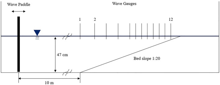
Layout of experiment of Mase and Kirby (1993).
The next data set used to analyze the performance of various frequency distribution functions is that of Bowen and Kirby (1994) (hereinafter BK94). BK94 performed an experiment to examine the behavior of random shoaling and breaking waves over a long beach slope. Of the three established wave conditions in the experiment, we use Case A and Case B where f p and H rms are 0.5 Hz and 7 cm, and 0.225 Hz and 8 cm, respectively. The wave conditions in Case A of BK94 correspond to intermediate water depth; that is, that of shallower water depth compared to Case 2 of MK93. Moreover, Case B of BK94 has a relative water depth at the peak frequency which is well within the shallow water range (k p h = 0.72 in Case A; k p h = 0.30 in Case B). The free surface elevation for BK94 was measured with a sampling rate of 25 Hz and was divided into 24 realizations of 1024 data points apiece. As in MK93, BK94 found the value of B and γ in β (Equation 3) as 1.15 and 0.6, respectively, and we assign the values in this study. The experimental layout showing 44 gauges along the 1:35 beach slope of a total of 47 gages appears in Figure 2. All three cases considered here in common have the random waves transforming and breaking over a plane beach of mild slope (i.e., 1:20 and 1:35), which might not violate the assumption of slowly varying bathymetry in the mild‐slope equation.
Figure 2.
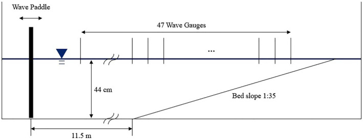
Layout of experiment Bowen and Kirby (1994).
3. Nonlinear Wave Model
3.1. Frequency‐Domain Model of Kaihatu and Kirby (1995)
Following Kaihatu and Kirby (1995) and Smith and Sprinks (1975) formulated a two‐dimensional parabolic nonlinear mild‐slope equation model in the frequency domain by applying Green's second identity to include quadratic nonlinear terms representing triad wave‐wave interaction between frequency components. And the one‐dimensional version of it is expressed by
| (9) |
where N is the total number of frequency components and and are
| (10) |
| (11) |
where ω is the wave angular frequency and two arbitrary frequency modes, l and n – l, interact with the nth frequency mode.
It is noted here that the amplitudes A n in Equation (9) are those of the free surface elevation but were derived from the first‐order dynamic free surface boundary condition connecting the velocity potential (the dependent variable of the original boundary value problem for water waves, and thus of the original mild slope equation) with the free surface elevation. Eldeberky and Madsen (1999) and Kaihatu (2001) showed how the resulting models underestimated the energy transfers at higher frequencies. To ameliorate these difficulties in the model of Kaihatu and Kirby (1995), Kaihatu (2001) included the second‐order relationship between potential function and surface elevation in the dynamic free surface boundary condition in the form of a correction:
| (12) |
where is the amplitude of free surface elevation complete with second order effects, and and are
| (13) |
| (14) |
3.2. Wave Breaking
The dissipation term for a bore‐type wave breaking α n is incorporated in the frequency‐domain model of Kaihatu and Kirby (1995), and the equation is solved using the Crank–Nicolson method to obtain a set of complex amplitudes at each location:
| (15) |
In this section, to revisit the effect of the frequency‐squared weighting on the spectra and higher‐order statistics in the random wave field, the values of F are chosen as either 0 or one in Equation (5). Then, F = 0 and F = 1 provide the frequency‐dependent dissipation term for the entire dissipation term and the frequency‐independent dissipation term, respectively:
| (16) |
with
| (17) |
Because the main purpose of the present study is to investigate the different frequency dependence functions of dissipation, the simple dissipation function of Thornton and Guza (1983) with shallow water approximation is used as the lumped dissipation term β (Equation 3) in the present study. Though wave setup was considered by using the balance of momentum flux (Longuet‐Higgins & Stewart, 1964) as a prescribed value rather than an iterative process in simulation, the wave setup had almost no effect on the results.
3.3. Deficiency of Previous Frequency Distribution Function
In order to detail a deficiency of the previous frequency distribution function, we here apply the frequency‐domain model of Kaihatu and Kirby (1995), with the frequency distribution function of Mase and Kirby (1993) to Case 2 of their experimental data. In order to assess the choice of the F value (i.e., F = 0 and 1), the dissipation terms for the nth frequency mode α n with F = 0 and F = 1 (see Equations 5 and 16) are thus used in computing spectrum and statistics. We are also to evaluate the influence of second‐order correction with Equation (12), the results with or without second‐order correction are also taken into consideration.
By using Fast Fourier Transform, we obtain sets of amplitudes A n from seven realizations of the time series for the water surface elevation at the upwave boundary. We then run the model of Equation (15) to calculate the complex amplitudes for each gauge and each realization and obtain the wave spectra at the location corresponding to the measurement location. Next, we obtain the time series of surface elevation with inverse Fourier transform on the calculated amplitudes A n . The obtained time series of water surface elevation η are processed to provide H rms and higher‐order moments such as skewness and asymmetry (see Equations 4, 7 and 8). To make use of the results for all realizations, Bartlett averaging is taken, and band averaging over nine adjacent bands is also used to smooth the spectrum and relieve the effect of noise. We use N = 400 as the total number of frequency components for Case 2 of MK93 since this retains a significant percentage of the spectral energy (99.92% at h = 47 cm).
Figures 3 and 4 show the results of spectra and higher‐order moments using N = 400 (i.e., H rms , skewness, and asymmetry), respectively. The results are consistent with the finding of MK93 that F = 0 destroyed the shape of the power spectrum at the shallowest gauge (Kirby & Kaihatu, 1997). Predictions of higher moments are significantly improved by the second‐order correction except for the asymmetry (Kaihatu, 2001). However, it is revealed that the existing frequency dissipation functions are not capable of accurately predicting the evolution of waves in the breaking zone. We will explain why the existing frequency distribution function (i.e., F = 0) leads to the destroyed shape of the spectrum at h = 2.5 cm (k p h = 0.32) and the asymmetry is still poorly predicted in detail in the next section.
Figure 3.

Comparison of wave spectra density using N = 400 for Case 2 of MK93: (a) h = 47 cm; (b) h = 30 cm; (c) h = 17.5 cm; (d) h = 10 cm; (e) h = 7.5 cm; (f) h = 2.5 cm (Solid: Data of MK93; Dashed: F = 0 without second order correction; Dotted: F = 1 without second order correction; Dash‐dot: F = 0 with s order correction; Solid‐x: F = 1 with s order correction).
Figure 4.

Comparison of higher‐order moments using N = 400 for Case 2 of MK93: (a) H rms ; (b) Skewness; (c) (Negative) Asymmetry (Open circle: Data of MK93; Dashed: F = 0 without second‐order correction; Dotted: F = 1 without second‐order correction; Dash‐dot: F = 0 with s‐order correction; Solid‐x: F = 1 with s‐order correction).
4. Frequency Dependence for Dissipation Coefficients
4.1. Intensity of Frequency Dependence for Dissipation Coefficient
The evolution of waves in the nearshore (or surf zone) results from such processes as shoaling, breaking, and nonlinear interactions. Neglecting depth change and nonlinear interactions, the relation between dissipation term α n and spectral density S n was presented by MK93:
| (18) |
where is the spectral density, and subscript x indicates x‐derivative. Using a forward difference method for x‐derivative of the spectrum (S nx ), the dissipation term of nth frequency mode α n is calculated with observed data at gauge:
| (19) |
where superscript i denotes the number of the gauge under consideration and Δx is the distance between gauges. When we use the measured data for , it contains not only shoaling effects but also nonlinear wave interactions, which conflict with the assumed condition to construct Equation (18) (i.e., shoaling effect and nonlinear interactions are neglected). Therefore, some revisions to the measured density at th gauge, is required to remove the shoaling effect and the effect of nonlinear wave interaction:
| (20) |
where is a calculated value by the frequency‐domain model of Kaihatu and Kirby (1995) without damping coefficient (i.e., Equation 9), using ith gauge measured data. Here is a spectral density at th gauge which is evolved only by the damping effect between two consecutive gauges (i.e., th gauge and th gauge) because the terms in the square bracket of Equation (20) refer to the effects of shoaling and nonlinear wave interaction between two gauges. Finally, the damping coefficient for the frequency mode n, α n can be provided with the combination of the measured spectral density at ith gauge and the revised one at th gauge:
| (21) |
Elgar et al. (1997) expressed the dissipation rate (not α n ) in a similar manner where the Boussinesq equation of Chen et al. (1997) was used to estimate nonlinear energy transfers (see Equation 5 of Elgar et al. [1997]). Figure 5 presents the calculation of α n using Equation (21) for Case 2 of MK93. When we calculate evolved only by the damping effect, it is significant to obtain accurate shoaling and nonlinear effects between two gauges (i.e., square bracket of Equation 20). However, as mentioned in the introduction section as well as in Chen et al. (1997), the nonlinearity is adjusted to maintain the preferred spectral shape if the dissipation function is not appropriately given (or, as in this case, missing altogether). In the simulation to calculate by using Equation (9) where the damping coefficient is not considered, the nonlinearity, therefore, becomes different in comparison to the nonlinear effect of which the dissipation function is involved in the equation (i.e., Equation 15). In order to minimize the differences between the nonlinear effects with and without the damping coefficients, following MK93, N = 300 (up to ) is used to calculate α n rather than N = 400 (up to ) used for the comparisons of spectra and higher‐order moments between model and the data of MK93. Otherwise, when we use N = 400 (not shown here), the nonlinear effects that are distorted to maintain the preferred spectra give rise to the negative values of α n at the shoaling regions (h = 10–17.5 cm) over the higher frequencies , which leads to a negative intensity of frequency dependence for α n over the regions. This is because the fewer frequency components (or smaller N) would probably reduce the differences in the nonlinear effects with or without the damping coefficients.
Figure 5.

Calculation of dissipation coefficients using Equation (21) and quadratic trend lines for Case 2 of MK93: (a), (b): h = 10–7.5 cm; (c), (d): h = 7.5–5 cm; (e), (f): h = 5–2.5 cm (Solid: calculated α n ; Dashed: quadratic trend lines).
The results from data of the four shallowest gauges, that is, the values of α n for the three intervals between gauges are shown in the left panels in Figure 5, corresponding to Figure 4b in MK93. In the right panels shown in Figure 5, the calculated α n is plotted against the trend lines (i.e., red dotted lines), of which form is a quadratic curve without the first‐order term (i.e., where b indicates a frequency‐independent portion). Since is the abscissa, the trends are depicted as straight lines, the slope (i.e., a in ) of which indicates an optimal intensity of dependence for α n , which is directly connected to the coefficients of corresponding to βδ in the case of F = 0 in the damping formulation of Mase and Kirby (1993) (see Equations 5 and 16 where b becomes zero in the case of F = 0 leading to entirely frequency‐weighted α n ):
| (22) |
We note here that the range of f n < 0.7 Hz is not taken into account when fitting these lines. The primary reason is that the frequency domain model treats the wave propagation problem as an initial value problem, and as such cannot account for wave reflection (Herbers et al., 2003). Since it is not possible to extract any wave reflection energy from the low frequency band (most impacted by reflection), energy in these bands is not used in the ensuing line fits. Otherwise, the effect of reflection over the range of f n < 0.7 Hz can be misinterpreted as a significant energy dissipation in the low frequency range, reducing the slope of the trendline and leading to an underestimated intensity of dependence for α n (see the left panels of Figure 5).
Here, we define the intensity of dependence for α n (corresponding to the slope of the red lines in the right panels of Figure 5) as the “intensity of frequency dependence” (IOFD) (i.e., a in ; e.g., βδ in Equation 22). In the damping coefficient outlined by MK93, the frequency dependence for α n is governed by parameters F, δ and coefficient β (i.e., ). In previous studies (e.g., Chen et al., 1997; Kaihatu & Kirby, 1995; Mase & Kirby, 1993), the value of F for the frequency dependent dissipation terms is constant for all gauges; representative values include F = 0 or F = 0.5 (Equation 22 is the expression with F = 0). Nonetheless, the coefficient β, which is multiplied by in Equation (22), rapidly increases at the shallower gauges because the term (H rms /h) in β is raised to the fifth power (see Equation 3). This is because , which represents the ratio of maximum height to water depth (H b /h) in β is set to constant, even for a saturated surf zone (in which H b /h approaches H rms /h). We note that when the constant is replaced with H rms /h for the saturated wave breaking conditions, β becomes less sensitive to the water depth. It is clear from the variation of the data‐derived dissipation coefficient values that the dissipation coefficients used in the models require less increase in IOFD with respect to the decreasing water depth, especially at the shallowest gauge where h = 2.5 cm and k p h = 0.32 (saturated surf zone where ).
A comparison of the values of IOFD from the data to those from Equation (22) (in which F = 0) is shown in Figure 6. It is clear that there is a strong deviation between optimal and predicted values of IOFD (i.e., IOFD from the data and IOFD with F = 0), with the former showing far more gradual variation with respect to water depth than the latter. Underprediction of this IOFD can be manifested in an underprediction in wave asymmetry (seen in Figure 4c), as the influence of frequency on the distribution of dissipation is necessary to lead to the high negative asymmetry seen in typical surf zone areas. Conversely, IOFD is overestimated with respect to the optimal values at the shallowest gauges (IOFD with F = 0 = 4.34; IOFD from data = 0.59 at h = 2.5 cm). The choice of F = 0 (full weighting of the dissipation distribution toward a frequency‐squared dependence) is the likely cause of this overprediction, as it aggressively dissipates energy from the high frequencies.
Figure 6.

Comparison of intensity of frequency dependence for dissipation coefficients in surf zone for Case 2 of MK93.
4.2. Modified Frequency Distribution Function
To optimize the frequency‐squared weighting of α n (i.e., the coefficient of in α n ) to the appropriate value of IOFD in the surf zone while still using the dissipation function (β) of Thornton and Guza (1983) as a basis, we suggest the following form of damping coefficient:
| (23) |
where β f is a new dissipation function to be used to constrain the frequency‐dependent dissipation, where the negative sign in front of β f in Equation (23) is used to allow α n to satisfy the following relation to ensuring that the total dissipation across the spectrum would be unaffected by the choice of frequency dependence (Equation 6).
The IOFD to be optimized is expressed as a coefficient multiplied by in α n , which corresponds to in the newly suggested term in Equation (23). In Figure 6, the data‐fitted value exponentially increases with decreasing water depth, but the fitted power function should have a power smaller than 5 to better reflect the trends seen in the data‐fitted coefficients. In reference to the existing form of β, which consists of the multiplication of free parameters and constants (i.e., ), , an exponential function with the base of H rms /h, and (see Equation 3), we suggest the following form of dissipation coefficient for the frequency dependent term:
| (24) |
where a free parameter B f is determined as 0.17 by using the least squares regression with the optimal intensities from the deepest gauge to the shallowest gauge for Case 2 of MK93. Note that the power of the term H rms /h is 2 rather than 5, in an attempt to reduce the dissipation function sensitivity to decreasing depth. Of possible candidates such as 0.5 to 5, power 2 provides the best‐fitting line for IOFD. Figure 6 compares the estimates of IOFD by the previous wave breaking coefficient with F = 0 and the newly developed damping coefficient to the values from data in the surf zone. In this section, it would be opportune to discuss the previous distribution function (Equation 5) with calibrated F as an alternative to that with F = 0 or 1. It was found that the optimal parameter F = 0.85 for Case 2 of MK93 through the same process of finding the parameter as for B f . However, compared to F = 1, F = 0.85 has nearly the same results regarding spectral transformation and higher‐order moment predictions. Hence, the results with F = 0.85 is not shown here for the sake of conciseness; for the results of skewness and asymmetry with the value of F between 0 and 1 (e.g., F = 0.25, 0.5, and 0.75), the reader is referred to Kaihatu and Kirby (1997) and Kaihatu (2001).
4.3. Comparison to Data of Mase and Kirby (1993)
We first confirm the performance of the new model by comparison with MK93, the data of which were used to help develop the model. We examine the performance of the newly proposed frequency distribution function by investigating the model predictions of wave spectrum (where a frequency resolution is Δf = 1/T and T is a record length of one realization), higher‐order moments (Equations 7 and 8), surface elevation η, and associated comparisons to data of MK93 using N = 400. In Section 3, the addition of the second‐order correction demonstrates a clear improvement, in particular for higher moments, and hence we present the second‐order corrected results by using Equation (12) with the various frequency distribution functions.
Figure 7 compares wave spectra between the different frequency distribution functions. The overall results show that the modified frequency distribution function provides improved predictions for high frequencies. As previously discussed for Case 2 of MK93 in Section 4.1, it can be seen at the gauge where the waves appear to begin dissipating (h = 17.5 cm, k p h = 0.95) that the correction by the present model for the underestimated intensity of weighting for α n leads to the improved agreement in wave spectrum for the high frequencies (see Figure 7c). Overall, however, one may conclude from comparisons between previous and present models that the modification has little effect on the predicted spectral densities. This is not surprising, since the predicted spectra are insensitive to the frequency dependence mainly due to the nonlinear effect which maintains the preferred spectral shape in the surf zone (Chen et al., 1997). Furthermore, the small impact of this correction on the evolution of spectral density can be attributed to the high relative water depth even at the shallowest gauge (k p h = 0.32 at h = 2.5 cm), since as the water becomes shallower, the waves are more likely to undergo by wave breaking. We can therefore hypothesize that the present model better predicts the evolution of the wave spectrum in the case of shallower water depth (i.e., with smaller k p h).
Figure 7.

Comparison of wave spectra density using N = 400 for Case 2 of MK93: (a) h = 47 cm; (b) h = 30 cm; (c) h = 17.5 cm; (d) h = 10 cm; (e) h = 7.5 cm; (f) h = 2.5 cm (Solid: Data of MK93; Dashed: Present model; Dotted: F = 0; Dash‐dot: F = 1).
Figure 8 compares the values of H rms and third moments (skewness and asymmetry) between results from present and previous models with values from measurement. As seen in Figure 6, the choice of F = 0 allows more dissipation for higher frequency components in the shallowest gauge than the modified dissipation. Nevertheless, this is surprising results that the present model generally agrees more with the negative values of asymmetry. In particular, at the shallowest gauge for Case 2 of MK93 (i.e., h = 2.5 cm), the present weighting represents the asymmetry accurately without the sudden decrease resulting from the excessive weighting in F = 0. Considering all the comparisons of the third moment, the present dissipation term is expected to predict more adequately the free surface elevation of breaking waves. However, since the present method still underestimates wave skewness considerably, the likely causes of these deleterious comparisons are detailed later in the section the discussion.
Figure 8.

Comparison of higher‐order moments using N = 400 for Case 2 of MK93: (a) H rms ; (b) Skewness; (c) (Negative) Asymmetry (Open circle: Data of MK93; Dashed: Present model; Dotted: F = 0; Dash‐dot: F = 1).
Figure 9 shows the time series from both models and laboratory measurements. These time series depict the most evident effect of the modification of the frequency distribution function. We note here that our primary intent is to compare wave shapes between time series, rather than the exact matching of time series. The predictions of asymmetry with the previous model with F = 1 (seen in Figure 8), which were the worst, seem to be in accordance with the mostly‐symmetric wave shape. As the previous studies suggest, F = 0 shows better agreement in wave shape than F = 1 with the exception at the gauge of h = 2.5 cm in Case 2 of MK93. The deleterious result of F = 0 at the shallowest measurement point is likely due to the frequency‐squared weighting of dissipation and is in accord with the shape of the wave spectrum shown in Figure 7f. Furthermore, we notice that the present dependence function provides better descriptions of a breaking wave train in the surf zone, which is consistent with the predictions of statistical third moments (asymmetry and skewness) in the wave shape pattern. In particular, the slopes of the front and rear faces are apparent, with a vertical front face and a gently sloping rear face (seen in the right panels in Figure 9), which is indicative of the improved asymmetry prediction by the present function.
Figure 9.
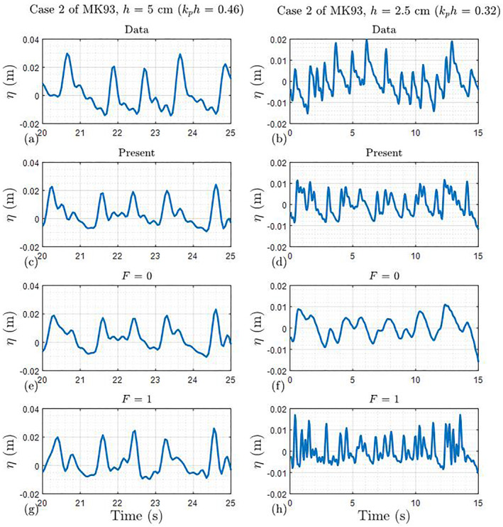
Comparison of free surface elevation using N = 400 for Case 2 of MK93: (a) Data at h = 5 cm; (b) Data at h = 2.5 cm; (c) Present model at h = 5 cm; (d) Present model at h = 2.5 cm; (e) F = 0 at h = 5 cm; (f) F = 0 at h = 2.5 cm; (g) F = 1 at h = 5 cm; (h) F = 1 at h = 2.5 cm.
5. Verification of the Model for Bowen and Kirby (1994)
As done in the previous section, we evaluate the performance of the new model by applying it to the experimental data of BK94, which serves as an independent validation since these data were not used for the development of the model. The experimental wave information for BK94 is shown in Table 1 and we use N = 150 since it also retains a significant percentage of the energy content in the spectrum. Note that we concern ourselves with the second‐order corrected results for all the models. As mentioned in the previous section, the cases of BK94 having smaller values of relative water depth at the peak frequency (i.e., k p h) are more likely to be influenced by the energy decay due to wave breaking. Therefore, the verification of the frequency dependence models against the experimental cases of BK94 can demonstrate the models' abilities in describing breaking waves.
Table 1.
Wave Information and Setup of Experiments
| Experiments | Bed slope | H rms (cm) | N | f p (Hz) | k p h | S 0 | γ b |
|---|---|---|---|---|---|---|---|
| Case 2 of MK93 | 1:20 | 4.7 | 400 | 1 | 1.97 | 0.03 | 0.81 |
| Case A of BK94 | 1:35 | 6.6 | 150 | 0.5 | 0.72 | 0.01 | 0.58 |
| Case B of BK94 | 1:35 | 7.7 | 150 | 0.225 | 0.30 | 0.003 | 0.44 |
Figures 10 and 11 show the comparisons between surface elevation wave spectra resulting from both the new and previous frequency distribution functions. Figures 12 and 13 compare the statistics from the measurements of BK94 and both the new and previous functions. We can see that the improvement by the modified model of this study is much more striking for cases of BK94 where the relative water depth is smaller than that of MK93. This is primarily due to the increasing influence of the bathymetry, resulting in breaking processes that are dominant over nonlinear wave interactions, which is supported by the fact that more significant improvements by present frequency dependence function are found in the shallower one of two cases of BK94 (i.e., best in Case B of BK94). Chen et al. (1997) confirmed that the frequency weighting functions did not have a critical effect on the shape of spectral density, however, it is clear that the modified frequency weighting for α n has a significant effect on the evolution of the spectral shape, especially at the shallowest gauges of two cases where the values of k p h are 0.27 and 0.12, respectively (see Figures 10f and 11f).
Figure 10.
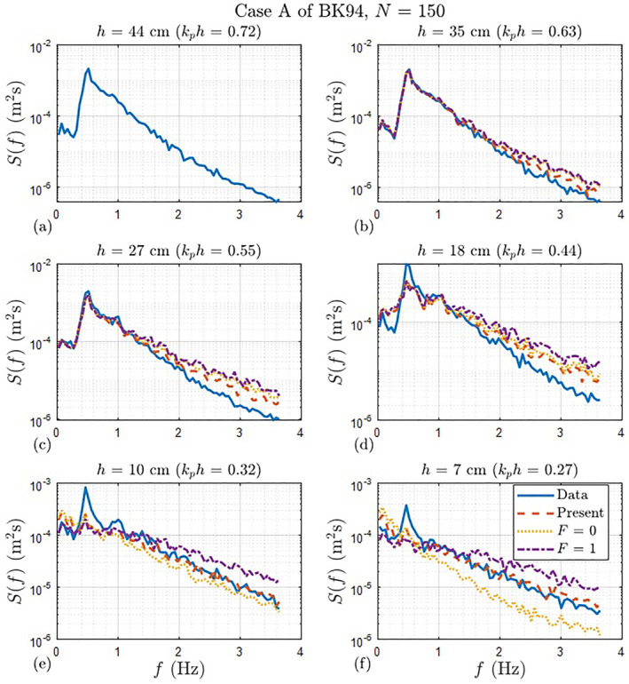
Comparison of wave spectra density using N = 150 for Case A of BK94: (a) h = 44 cm; (b) h = 35 cm; (c) h = 27 cm; (d) h = 18 cm; (e) h = 10 cm; (f) h = 7 cm (Solid: Data of MK93; Dashed: Present model; Dotted: F = 0; Dash‐dot: F = 1).
Figure 11.

Comparison of wave spectra density using N = 150 for Case B of BK94: (a) h = 44 cm; (b) h = 35 cm; (c) h = 27 cm; (d) h = 18 cm; (e) h = 10 cm; (f) h = 7 cm (Solid: Data of MK93; Dashed: Present model; Dotted: F = 0; Dash‐dot: F = 1).
Figure 12.
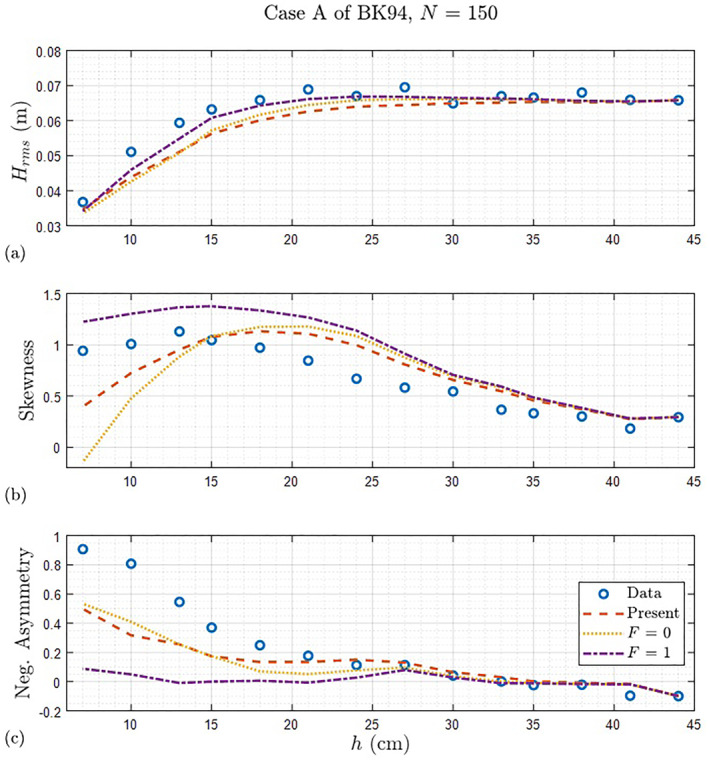
Comparison of higher‐order moments using N = 150 for Case A of BK94: (a) H rms ; (b) Skewness; (c) (Negative) Asymmetry (Open circle: Data of MK93; Dashed: Present model; Dotted: F = 0; Dash‐dot: F = 1).
Figure 13.

Comparison of higher‐order moments using N = 150 for Case B of BK94: (a) H rms ; (b) Skewness; (c) (Negative) Asymmetry (Open circle: Data of MK93; Dashed: Present model; Dotted: F = 0; Dash‐dot: F = 1).
Figures 14 and 15 present parts of the temporal variations of free surface elevations by the present and previous models with the observed counterpart. We note that the effect of the present frequency dependence in the dissipation function is manifested in the differences in wave shape relative to those from previous formulations. Two features are apparent in the present model: (a) while the dependence with F = 1 depicts a waveform with small fluctuating waves, the present modified dependence reduces the excessive perturbations and (b) the time series of the present model shows steep front and gradual rear faces (saw‐toothed shape), especially shown in the right panels of Figure 15, which is directly connected to the well predicted asymmetry by the present function. To sum up, the modified frequency dependence of this study is the most representative, which is not surprising, since it has the best predictions of wave shape statistics as well as wave spectrum for all cases of experiment.
Figure 14.

Comparison of free surface elevation using N = 150 for Case A of BK94: (a) Data at h = 10 cm; (b) Data at h = 7 cm; (c) Present model at h = 10 cm; (d) Present model at h = 7 cm; (e) F = 0 at h = 10 cm; (f) F = 0 at h = 7 cm; (g) F = 1 at h = 10 cm; (h) F = 1 at h = 7 cm.
Figure 15.
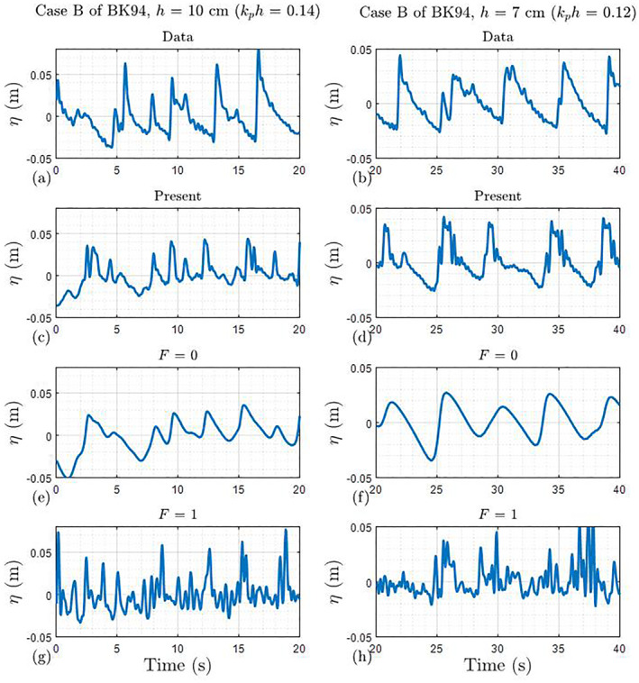
Comparison of free surface elevation using N = 150 for Case B of BK94: (a) Data at h = 10 cm; (b) Data at h = 7 cm; (c) Present model at h = 10 cm; (d) Present model at h = 7 cm; (e) F = 0 at h = 10 cm; (f) F = 0 at h = 7 cm; (g) F = 1 at h = 10 cm; (h) F = 1 at h = 7 cm.
6. Discussion
In the present work, we introduced the intensity of frequency dependence for wave breaking function to appropriately account for the dissipation in breaking waves. The overall agreement between predictions and measurements is good and the improvements on account of the modified frequency distribution function are considerable. However, there are still considerable discrepancies, particularly in skewness and asymmetry for both experimental data. There are several possible reasons for this.
One likely reason involves the practical aspects of nonlinear frequency domain modeling: the establishment of a limit on the number of frequencies modeled, which is generally well below the Nyquist frequency of the input data. The simplest criterion for this limit is computational time and stability; however, other criteria (the validity of the nonlinear terms and/or the breaking formulation at high frequencies) may also be relevant. However, it is established, the net effect of the upper‐frequency limit impacts third‐moment estimates. The Fourier representation of ocean surface waves is limited by the Nyquist frequency, a function of the sampling rate of the measurement. Even if the cutoff frequency established for the model was also applied to the data (in both input forcing and model – data comparisons), wave‐wave interactions up to the Nyquist limit have impacted the measured waves across the entire frequency range. As previously stated, the relatively poor results in the spectral densities over the low frequency range may be due to the limitation of a frequency‐domain model in that the effect of wave reflection (or, in the case of wave tank experiments, re‐reflection) cannot be simulated, which would likely to result in the deleterious comparisons in the wave shape statistics.
Another possible reason would be related to the parameters set to constant in the wave breaking function. The parameter γ in the wave breaking function β relating the maximum wave height before breaking to water depth remains constant in the saturated surf condition. The use of constant parameter γ in the over‐saturated surf zone can induce the distribution of breaking wave height for all waves that is greater than one (i.e., ), which possibly yields the overestimated dissipation over the entire range of frequency as well as the high‐frequency range. Secondly, since the experimental cases of BK94 were used to verify the breaking model using B f = 0.17 developed with the case of MK93, we did not consider the optimized value of B f for both cases of BK94. Although it is not detailed in this paper for brevity, it was determined that the optimal parameters B f for BK94 are greater than that for MK93: 0.23 and 0.36 for Case A and Case B in BK94, respectively. The optimal parameter B f is likely to increase as the case is more affected by the breaking‐induced energy dissipation. Therefore, it is anticipated that the use of optimized B f for each case better follows the trend of the data. As a suggestion for the extension of this study, the analysis of IOFD with other cases in experimental and field environments should be performed to find the calibration coefficients β f fit for each case.
7. Conclusions
Kirby et al. (1992) and Mase and Kirby (1993) first formulated the frequency‐dependent damping coefficient for breaking dissipation consisting of two terms: (a) a frequency‐independent term which drains energy over all frequencies and (b) an entirely frequency‐squared weighted term. Following the deduction process by Mase and Kirby (1993), we propose a new form of frequency dependent dissipation term with Case 2 of MK93. We, however, introduce different dissipation functions for the frequency independent and dependent portions (i.e., β and β f ) to consider the change of intensity of frequency dependence with the decrease in water depth. This is in contrast to Mase and Kirby (1993), who used the identical dissipation function for the frequency‐independent and dependent term (i.e., β).
The frequency dependence of wave‐breaking‐induced dissipation is investigated by comparing predictions of frequency‐domain models with laboratory data of MK93 and BK94. In addition to the energy spectra and statistical moments, the agreement between the predictions and the observations confirms the improved predictions resulting from the newly proposed function against the wave shape‐related characteristics such as the free surface elevation and the geometric asymmetry. Although the distributed energy dissipation by the choice of F has little impact on the spectral evolution (Chen et al., 1997; Kaihatu, 2001), the new formulation of the dissipation model in this study works reasonably better for the power spectrum, the improvement of the prediction of which becomes more apparent in the shallower cases.
Considering the geometric measures as well as statistical measures, Case B of BK94 is most demonstrative of the advantages of the modification in wave‐breaking‐induced dissipation. This case has the greatest H rms as well as the smallest γ b (see Table 1) resulting in the smallest breaking wave height H b , where the free parameter γ b is related to the breaking wave height H b , proposed by Battjes and Stive (1985):
| (25) |
where S 0 implies the offshore wave steepness, given by
| (26) |
where H rms,0 is H rms in deep water, and L p,0 denotes the wavelength at peak frequency in deep water. Consequently, Case B of BK94 is the most affected case by dissipation of wave breaking, which is the likely cause of the most improved results of all cases. It is also confirmed from the report by Bowen and Kirby (1994) that Case B has lost more energy during the breaking mechanism than Case A.
Acknowledgments
The first author was supported by a Doctoral Fellowship from the Zachry Department of Civil & Environmental Engineering at Texas A&M University. The work was also partly supported by Grant P42 ES027704 from the National Institute of Environmental Health Sciences.
Kim, I.‐C. , & Kaihatu, J. M. (2022). A modified frequency distribution function of wave breaking‐induced energy dissipation. Journal of Geophysical Research: Oceans, 127, e2022JC018792. 10.1029/2022JC018792
Data Availability Statement
The code and data that support the findings of this study are openly available at https://doi.org/10.5281/zenodo.6977660 repository.
References
- Alsina, J. M. , & Baldock, T. E. (2007). Improved representation of breaking wave energy dissipation in parametric wave transformation models. Coastal Engineering, 54(10), 765–769. 10.1016/j.coastaleng.2007.05.005 [DOI] [Google Scholar]
- Ardani, S. , & Kaihatu, J. M. (2019). Evolution of high frequency waves in shoaling and breaking wave spectra. Physics of Fluids, 31(8), 087102. 10.1063/1.5096179 [DOI] [Google Scholar]
- Baldock, T. , Holmes, P. , Bunker, S. , & Van Weert, P. (1998). Cross‐shore hydrodynamics within an unsaturated surf zone. Coastal Engineering, 34(3–4), 173–196. 10.1016/s0378-3839(98)00017-9 [DOI] [Google Scholar]
- Battjes, J. A. , & Janssen, J. (1978). Energy loss and set‐up due to breaking of random waves. In Coastal Engineering 1978 (pp. 569–587).
- Battjes, J. A. , & Stive, M. (1985). Calibration and verification of a dissipation model for random breaking waves. Journal of Geophysical Research, 90(C5), 9159–9167. 10.1029/jc090ic05p09159 [DOI] [Google Scholar]
- Booij, N. , Ris, R. C. , & Holthuijsen, L. H. (1999). A third‐generation wave model for coastal regions: 1. Model description and validation. Journal of Geophysical Research, 104(C4), 7649–7666. 10.1029/98jc02622 [DOI] [Google Scholar]
- Bowen, G. D. , & Kirby, J. T. (1994). Shoaling and breaking random waves on a 1: 35 laboratory beach. University of Delaware, Department of Civil Engineering, Center for Applied Coastal Res. [Google Scholar]
- Chen, Y. , Guza, R. , & Elgar, S. (1997). Modeling spectra of breaking surface waves in shallow water. Journal of Geophysical Research, 102(C11), 25035–25046. 10.1029/97jc01565 [DOI] [Google Scholar]
- Chen, Y. , & Liu, P. L. F. (1995). Modified Boussinesq equations and associated parabolic models for water wave propagation. Journal of Fluid Mechanics, 288, 351–381. 10.1017/s0022112095001170 [DOI] [Google Scholar]
- Eldeberky, Y. , & Battjes, J. A. (1996). Spectral modeling of wave breaking: Application to Boussinesq equations. Journal of Geophysical Research, 101(C1), 1253–1264. 10.1029/95jc03219 [DOI] [Google Scholar]
- Eldeberky, Y. , & Madsen, P. A. (1999). Deterministic and stochastic evolution equations for fully dispersive and weakly nonlinear waves. Coastal Engineering, 38(1), 1–24. 10.1016/s0378-3839(99)00021-6 [DOI] [Google Scholar]
- Elgar, S. , Guza, R. , Raubenheimer, B. , Herbers, T. , & Gallagher, E. L. (1997). Spectral evolution of shoaling and breaking waves on a barred beach. Journal of Geophysical Research, 102(C7), 15797–15805. 10.1029/97jc01010 [DOI] [Google Scholar]
- Herbers, T. , Orzech, M. , Elgar, S. , & Guza, R. (2003). Shoaling transformation of wave frequency‐directional spectra. Journal of Geophysical Research, 108(C1), 3013. 10.1029/2001jc001304 [DOI] [Google Scholar]
- Janssen, T. T. , & Battjes, J. (2007). A note on wave energy dissipation over steep beaches. Coastal Engineering, 54(9), 711–716. 10.1016/j.coastaleng.2007.05.006 [DOI] [Google Scholar]
- Kaihatu, J. M. (2001). Improvement of parabolic nonlinear dispersive wave model. Journal of Waterway, Port, Coastal, and Ocean Engineering, 127(2), 113–121. 10.1061/(asce)0733-950x(2001)127:2(113) [DOI] [Google Scholar]
- Kaihatu, J. M. , & Kirby, J. T. (1995). Nonlinear transformation of waves in finite water depth. Physics of Fluids, 7(8), 1903–1914. 10.1063/1.868504 [DOI] [Google Scholar]
- Kaihatu, J. M. , & Kirby, J. T. (1997). Effects of mode truncation and dissipation on predictions of higher order statistics. In Coastal Engineering 1996 (pp. 123–136).
- Kaihatu, J. M. , Veeramony, J. , Edwards, K. L. , & Kirby, J. T. (2007). Asymptotic behavior of frequency and wave number spectra of nearshore shoaling and breaking waves. Journal of Geophysical Research, 112(C6), C06016. 10.1029/2006jc003817 [DOI] [Google Scholar]
- Kirby, J. T. , & Kaihatu, J. M. (1997). Structure of frequency domain models for random wave breaking. In Coastal Engineering 1996 (pp. 1144–1155).
- Kirby, J. T. , Kaihatu, J. M. , & Mase, H. (1992). Shoaling and breaking of random wave trains: Spectral approaches (pp. 71–74). Engineering Mechanics. [Google Scholar]
- Longuet‐Higgins, M. S. , & Stewart, R. (1964). Radiation stresses in water waves; a physical discussion, with applications, paper presented at Deep sea research and oceanographic abstracts. Elsevier. [Google Scholar]
- Madsen, P. , & Sørensen, O. (1993). Bound waves and triad interactions in shallow water. Ocean Engineering, 20(4), 359–388. 10.1016/0029-8018(93)90002-y [DOI] [Google Scholar]
- Mase, H. , & Kirby, J. T. (1993). Hybrid frequency‐domain KdV equation for random wave transformation. In Coastal Engineering 1992 (pp. 474–487).
- Smith, J. M. , & Vincent, C. L. (2003). Equilibrium ranges in surf zone wave spectra. Journal of Geophysical Research, 108(C11), 3366. 10.1029/2003jc001930 [DOI] [Google Scholar]
- Smith, R. , & Sprinks, T. (1975). Scattering of surface waves by a conical island. Journal of Fluid Mechanics, 72(2), 373–384. 10.1017/s0022112075003424 [DOI] [Google Scholar]
- Thornton, E. B. , & Guza, R. (1983). Transformation of wave height distribution. Journal of Geophysical Research, 88(C10), 5925–5938. 10.1029/jc088ic10p05925 [DOI] [Google Scholar]
- Whitford, D. J. (1988). Wind and wave forcing of longshore currents across a barred beach. Naval Postgraduate School. [Google Scholar]
Associated Data
This section collects any data citations, data availability statements, or supplementary materials included in this article.
Data Availability Statement
The code and data that support the findings of this study are openly available at https://doi.org/10.5281/zenodo.6977660 repository.