

Abstract
Current-Clamp electroporation refers to the application of a constant current across a membrane which results in voltage fluctuations due to the creation of electropores. This method allows for the measurement of electroporation across a long timescale (minutes) and facilitates the comparison between experimental and theoretical studies. Of particular interest is the claim in the literature that current-clamp electroporation results in the creation of a single pore. We simulated current-clamp electroporation using the Smoluchowski and Langevin equations and identified two possible mechanisms to explain the observed voltage fluctuations. The voltage fluctuations may be due to a single pore or a few pores growing and shrinking via a negative feedback mechanism or the opening and closing of pores in a larger population of pores. Our results suggest that current-clamp conditions do not necessarily result in the creation of a single pore. Additionally, we showed that the Langevin model is more accurate than the Smoluchowski model under conditions where there are only a few pores.
Keywords: Electroporation, Chronopotentiometry, Smoluchowski, Langevin, Hopf Bifurcation
1. Introduction
Electroporation refers to the general phenomenon of the creation of transient pores in lipid membranes in response to an applied electric field. In the biomedical sciences, electroporation is used primarily for tumor ablation, drug delivery, and gene delivery [1]. Since the size of electropores is very small (nanometers), and the timescale of their creation and growth is very short (nanoseconds) [2], they are difficult to observe directly using microscopy. Recently, optical single-channel recordings have been used to visualize electropores in droplet interface bilayers with a time resolution of 16 ms [3]. Indirect experimental methods probing membrane conductivity [4], molecular uptake [5,6], and gene expression [7] have often been used to gain a better understanding of electroporation. However, using these methods alone tells us little about the biophysical processes involved in electroporation.
Continuum models and molecular dynamics simulations have been the two main approaches used to gain a better theoretical understanding of electroporation [8]. Although they represent two fundamentally different approaches, both show surprising qualitative agreement with respect to the mechanism of electroporation [8]. The continuum theory posits that in response to an applied electric field, pores are initially created as small, cylindrical, hydrophobic pores, and then are stabilized into larger, toroidal, hydrophilic pores [8]. The theoretical transition between hydrophobic pores and hydrophilic pores has also been observed in molecular dynamics simulations [8–10].
A popular continuum model, the Smoluchowski model, is a partial differential equation (PDE) which governs the distribution of pores with respect to their size and with respect to time. It has been used extensively in the electroporation literature for modeling experimental scenarios involving short nanosecond to millisecond electrical pulses [11–15]. A limitation of the model is that it uses a large number of parameters, many of which cannot be measured experimentally [2,16]. Another limitation, which has not been mentioned in the literature, is the fact that it treats pores as a continuous pore density, when in reality pores exist at discrete radii. In this work we show that the Smoluchowski model creates an artificial smoothing which becomes more obvious at lower pore number. For this reason, we also use an analogous Langevin model and compare our results. In this work, the Langevin model refers to a system of stochastic differential equations (SDE), which governs the sizes of individual pores. The Langevin model uses a separate SDE for each pore, so it does not suffer from the same artificial smoothing as the Smoluchowski model, but a limitation is that it can become computationally expensive for scenarios involving many pores.
In order to further validate results from models and simulations, comparisons with experimental data must also be made. In the past, good quantitative agreement has been shown between the continuum Smoluchowski electroporation model and experimental data of fluorescent dye uptake during electroporation [5,6,14]. However, almost all experimental and computational studies have focused on the case of high applied electric field strength, in which case a large number of pores are created [2,5,6,12–14,17,18]. Some experimental studies have shown that when artificial lipid bilayers are clamped at a low voltage, a single pore can be observed [3,4]. Others have claimed that the voltage fluctuations observed under current-clamp conditions also reflect the presence of a single electropore that fluctuates in size due to a negative feedback mechanism [19–25]. By clamping the current or voltage, and by having a single pore as opposed to a large population of pores, we greatly simplify the comparison between experimental and computational studies. In this work, we use the Smoluchowski model, and an analogous Langevin model to study electroporation under current-clamp conditions. We show that the voltage fluctuations observed under current-clamp conditions may either reflect a negative feedback mechanism involving a single pore, multiple pores, or a mechanism involving the creation and destruction of pores in a larger population of pores.
2. Theory and methods
2.1. Electroporation theory
In continuum electroporation models, pores are fully characterized by their radius, which is in turn determined by the pore energy landscape (Fig. 1). The pore energy at a given radius is defined as the lesser of and , the hydrophilic and hydrophobic pore energies respectively. Since only hydrophilic pores are considered to be conducting [2], we will only consider the hydrophilic pore energy and assume pores are created with a minimum radius . In this work we adopt the pore energy model described in Smith [14], which is based off of earlier models [12,13,17,18,26].
| (1) |
Fig. 1.

Pore Energy Landscape r* = 0.65 nm, B = 2 × 10⁻¹⁹ J, b = 2.5, γ = 0.8 × 10⁻¹¹ J m−1.
In Eq. (1), the first term represents the energy due to the steric repulsion of lipid heads, the second term is the edge energy, the third term is the interfacial energy, and the last term is the electrical energy [27]. All parameter names and values are given in Table 1. The effective surface tension, , is given by
| (2) |
to account for the fact that the creation of pores results in a change of the total lipid area, , which results in the change of the overall surface tension [14,28].
Table 1.
All Parameter value names, values and sources.
| Parameter | Value(s) | Definition and source |
|---|---|---|
|
| ||
| a | 104, 105 (m−2 s) | Pore creation rate density |
| β | 15 kT, 90 kT | Pore creation constant |
| σ | 1.2 S m−1 | Conductivity of electrolyte buffer (0.1 M KCl) [14] |
| Am | 9 × 10⁻⁶ m2 | Membrane area* [23] |
| Cm | 2.2 × 10⁻² F m−2 | Surface capacitance of the membrane* |
| Rm | 10 kΩ m2 | Surface resistance of the membrane [29] |
| h | 5 nm | Membrane thickness [14] |
| D | 10−18, 7 × 10⁻¹³ (m2 s−1) | Diffusion coefficient for pore radius |
| γ | 1.8 × 10⁻¹¹, 0.8 × 10⁻¹¹ (J m−1) | Edge energy [18] |
| Γ0 | 1 × 10⁻⁵ J m−2 | Membrane tension [14] |
| Γ’ | 2 × 10⁻² J m−2 | Tension of hydrocarbon-water interface [14] |
| Fmax | 0.70 × 10⁻⁹ N V−2 | Maximum electric force for Vm = 1 V [18] |
| rh | 0.97 × 10⁻⁹ m | Constant in eq. (1) [18] |
| rt | 0.31 × 10⁻⁹ m | Constant in eq. (1) [18] |
| r * | 0.65 × 10⁻⁹ m | Minimum hydrophilic pore radius [14] |
| T | 293 K | Absolute Temperature [23] |
| B | 1.48 × 10⁻¹⁹, 2 × 10⁻¹⁹ (J) | Steric Repulsion Constant |
| b | 3.6, 2.5 | Steric Repulsion Constant |
| a1 | −1.2167 | Coefficient in eq. (7) [14] |
| a2 | 1.5336 | Coefficient in eq. (7) [14] |
| a3 | −22.5083 | Coefficient in eq. (7) [14] |
| a4 | −5.6117 | Coefficient in eq. (7) [14] |
| a5 | −0.3363 | Coefficient in eq. (7) [14] |
| a6 | −1.216 | Coefficient in eq. (7) [14] |
| a7 | 1.647 | Coefficient in eq. (7) [14] |
| rs | 0.175 × 10⁻⁹ m | Potassium Radius [14] |
| n | 0.25 | Pore relative entrance length [14] |
The reduction of lipid area due to a single toroidal pore, , is given as [14]
| (3) |
where is the membrane thickness. Note that under conditions where a single pore is created, the lipid area does not change significantly, so the effective surface tension can be treated as a constant. As the transmembrane voltage changes during electroporation, the shape of the pore energy landscape is expected to change. At low voltages, a local minimum exists around , but disappears as the voltage increases, leading to irreversible electroporation (Fig. 1). However, if a single pore is created under voltage-clamp conditions, the pore energy landscape is expected to be static.
In this work we also adopt the pore conductance model described by Smith [14]. The pore resistance is given by
| (4) |
where is the conductivity of the solution, is the pore area, is the Hindrance factor, and is the Partition factor. The Hindrance factor for spherical solutes is given by
| (5) |
where is the solute radius and
| (6) |
where and the constants are included in Table 1. In this work we only consider the potassium ion whose radius is listed in Table 1. The Partition factor for a trapezoidal pore is given by [30]
| (7) |
where is the Born energy for a toroidal pore given by [14]
| (8) |
The Hindrance and Partition factors are necessary to account for the fact that the conductivity inside the pore is different from the bulk conductivity. The Hindrance factor arises from the steric hindrance due to the finite size of the solute with respect to the pore, and the frictional resistance or drag which results from the interaction of the solute with the pore walls [14,31]. The Partition factor arises from considerations involving the energetic cost to place a charge inside a pore [14,30].
Consider the flux of pores with respect to their radii consisting of diffusion due to thermal fluctuations and drift due to the action of a generalized force, , which is the gradient of the pore energy.
| (9) |
Eq. (9) is analogous to the drift–diffusion of a particle in a one-dimensional space. If Eq. (10) is combined with the equation of continuity,
| (10) |
we recover the Smoluchowski equation (Eq. (11)).
| (11) |
The Smoluchowski equation is a partial differential equation (PDE) which governs the evolution of pores. Note that is the pore density distribution such that there are pores with radii between and at time . Eq. (11) must be supplemented with an ordinary differential equation (ODE) describing the dynamics of the transmembrane voltage. For planar lipid membranes under current-clamp conditions, we use the following equation and initial condition
| (12) |
where is the capacitive current, is the applied constant current ( is the current density), is the current through pores, and is the leakage current. Note that and .
The total current through pores, , is given by
| (13) |
where is the maximum radius considered in the model.
While the Smoluchowski equation works well for cases with a large number of pores, it introduces an artificial smoothing when there are only a few pores. The Smoluchowski equation assumes a continuous pore density, when in reality, pores exist at discrete radii. For this reason, we also conduct simulations with the Langevin equation. In the limit of strong friction, the inertia term can be neglected, and the Langevin equation becomes
| (14) |
where is the friction coefficient, is the external force, and is the noise term. Using Einstein’s relation, we identify as the friction coefficient, and using the fluctuation–dissipation theorem, we identify as the fluctuation amplitude [32]. After substituting terms and rearranging, we arrive at the equation
| (15) |
where we simply take to be a gaussian white noise. This form of the Langevin equation is the stochastic analog of the Smoluchowski equation. By using the Langevin equation, we are able to uncover behavior that is hidden by the artificial smoothing of the Smoluchowski equation.
2.2. Numerical methods
To solve the Smoluchowski PDE, we adopt the numerical scheme described in Smith et al. [14,15]. Briefly, we use a method of lines (MOL) approach to solve the system involving the Smoluchowski PDE (Eq. (11)), and the ODE governing the transmembrane voltage (Eq. (12)). The spatial dimension of Eq. (11) is discretized as
| (16) |
where
| (17) |
is the discretized pore flux [14,15]. To describe the creation and destruction of pores we use the following boundary condition at.
| (18) |
where is the creation flux,
| (19) |
and is the destruction flux which is obtained by using an imaginary node at and setting the corresponding pore density to zero [14]. For the boundary at , we use an absorbing boundary condition by setting the corresponding time derivative to zero. The resulting system of ordinary differential equations is solved using MATLABs ode15s solver. At each time step, the pore energies, total lipid area, effective surface tension, and total current through pores are computed, and the boundary conditions are enforced. The value for was chosen to be high enough (0.1 mm) so that the pore density would be negligible near at and so that there would be no artificial restrictions on pore growth. The spatial coordinate (pore radius) was discretized using a step size of from 0.65 nm to 3 nm. The step size was linearly increased in increments of 1pm until r = 10nm, after which the radius was increased logarithmically until using 100 nodes.
For simulations using the Langevin Equation, we created a stochastic differential equation object for Eqs. (12) and (15) using MATLAB’s sde() function, and simulated using the simByEuler() function with a time-step of 1 μs. Pore creation and destruction was simulated in a way analogous to Eqs. (18) and (19). In particular, every millisecond, the number of pores created was computed using Eq. (19). Pores were “launched” by adding copies of Eq. (15) to the sde object with an initial condition of r*. Similarly, pores were destroyed by deleting copies of Eq. (15) from the sde object whenever a pore radius fell below a value of r* −1pm.
3. Results
We simulated current-clamp electroporation using the Smoluchowski equation, and tried to fit the experimental data from Fig. 2 of Naumowicz et al. [23] by adjusting the values of the diffusion coefficient D in Eq. (11), the pore creation parameters a and β, edge energy γ, and the steric repulsion constants B and b in Eq. (1). We identified two possible mechanisms which can explain the observed voltage fluctuations.
Fig. 2.
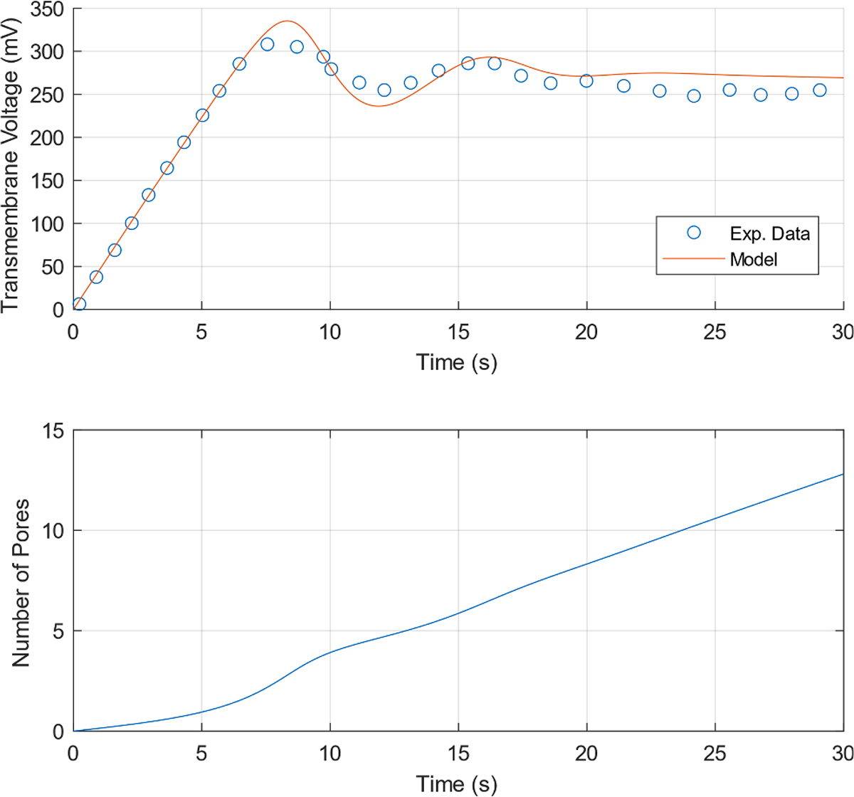
(Smoluchowski model) Current-Clamp Electroporation (j = 1 mA m−2). (Top) Transmembrane Voltage response and Exp. data from Naumowicz et al. [23] reproduced using the Engauge Digitizer Software [33]. (Bottom) Number of Pores as a function of time.
First, the voltage fluctuations may be a result of a negative feedback mechanism as suggested in Naumowicz et al. [23]. In particular, as the transmembrane voltage increases, the local minimum in the pore energy landscape disappears (Fig. 1) leading to pore expansion, which in turn causes a drop in the voltage, at which point the local minimum reappears and the pores begin to shrink. By using the parameter values a = 105, β = 15 kT, D = 10−18, γ = 0.8 × 10⁻¹¹, B = 2 × 10⁻¹⁹, and b = 2.5, we were able to achieve good fit with the experimental data. The transmembrane voltage and number of pores are shown as a function of time in Fig. 2 below. Videos of the spatiotemporal evolution of the pore density and the pore energy landscape are included in the Supplementary Material (S1).
To study the system more closely, we considered the case where there is a single pore present by solving the system involving Eq. (12) and Eq. (15) without the noise term. The corresponding phase-plane portrait assuming the presence of a single pore is shown in Fig. 3. Videos of the transmembrane voltage response and the spatiotemporal evolution of the pore energy landscape are included in the Supplementary Material (S2). In Fig. 3 (top), we observed the same damped oscillations which appear in the experimental data, but we were not able to achieve a good fit with the data. The pore reached an equilibrium value of 16 nm at a stable fixed point corresponding to a local maximum in the free energy landscape. Notably, by changing the value of the applied current density from j = 1 mA m−2 to j = 0.5 mA m−2, a limit cycle appears, indicating the presence of a Hopf Bifurcation.
Fig. 3.
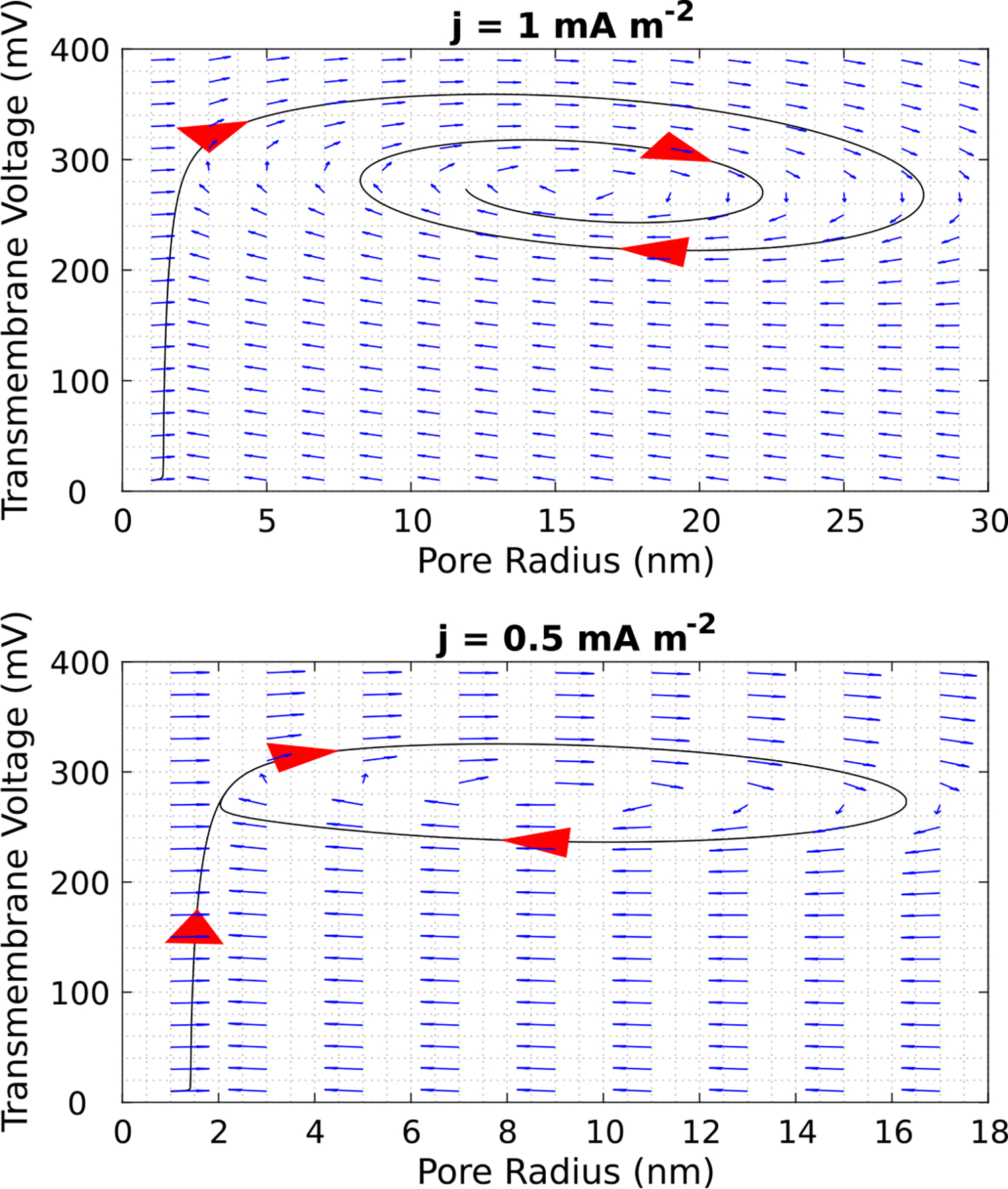
Phase Portraits of system from Fig. 2, assuming the presence of a single pore. Initial Condition: (Vm, r) = (0.01 V, 1 nm). Decreasing the current density from j = 1 mA m−2 to j = 0.5 mA m−2 reveals the presence of a Hopf Bifurcation.
We also simulated the system using the Langevin equation. This allowed us to look at the evolution of the radii of individual pores, and to avoid any unrealistic smoothing caused by the Smoluchowski equation. The transmembrane voltage, average pore radius, and selected pore radii are shown as a function of time in Fig. 4. Note how the voltage fluctuates for t > 20 s, in a way which is not noticeable in Fig. 2. This is due to current fluctuations caused by stochastic pore fluctuations. A comparison of the current through electropores predicted by the Smoluchowski and Langevin equations is shown in Fig. 5.
Fig. 4.

(Langevin model) Current-Clamp Electroporation (j = 1 mA m−2). (Left) Transmembrane Voltage response and Exp. data from Naumowicz et al. [23] reproduced using the Engauge Digitizer Software [33]. (Middle) Average Pore Radius over time. (Right) Radii of 3 selected pores over time.
Fig. 5.

Comparison of current through pores according to Langevin and Smoluchowski equations.
Alternatively, the voltage fluctuations may be a result of the opening and closing of pores in a population of pores. In particular, as pores are created the transmembrane voltage drops, and as they reseal the voltage rises, resulting in voltage fluctuations. Eventually, the rate of pore creation and destruction balances and the system reaches equilibrium. By using the parameter values a = 104, β = 90 kT, D = 7 × 10⁻¹³, γ = 1.8 × 10⁻¹¹, B = 1.48 × 10⁻¹⁹, and b = 3.6 in the Smoluchowski model, we were able to achieve good fit with the experimental data. The transmembrane voltage and number of pores are shown as a function of time in Fig. 6. Videos of the spatiotemporal evolution of the pore density and the pore energy landscape are included in the Supplementary Material (S3). We did not simulate this case using the Langevin equation due to the very high computational cost associated with simulating a large number of pores with a high diffusion coefficient.
Fig. 6.
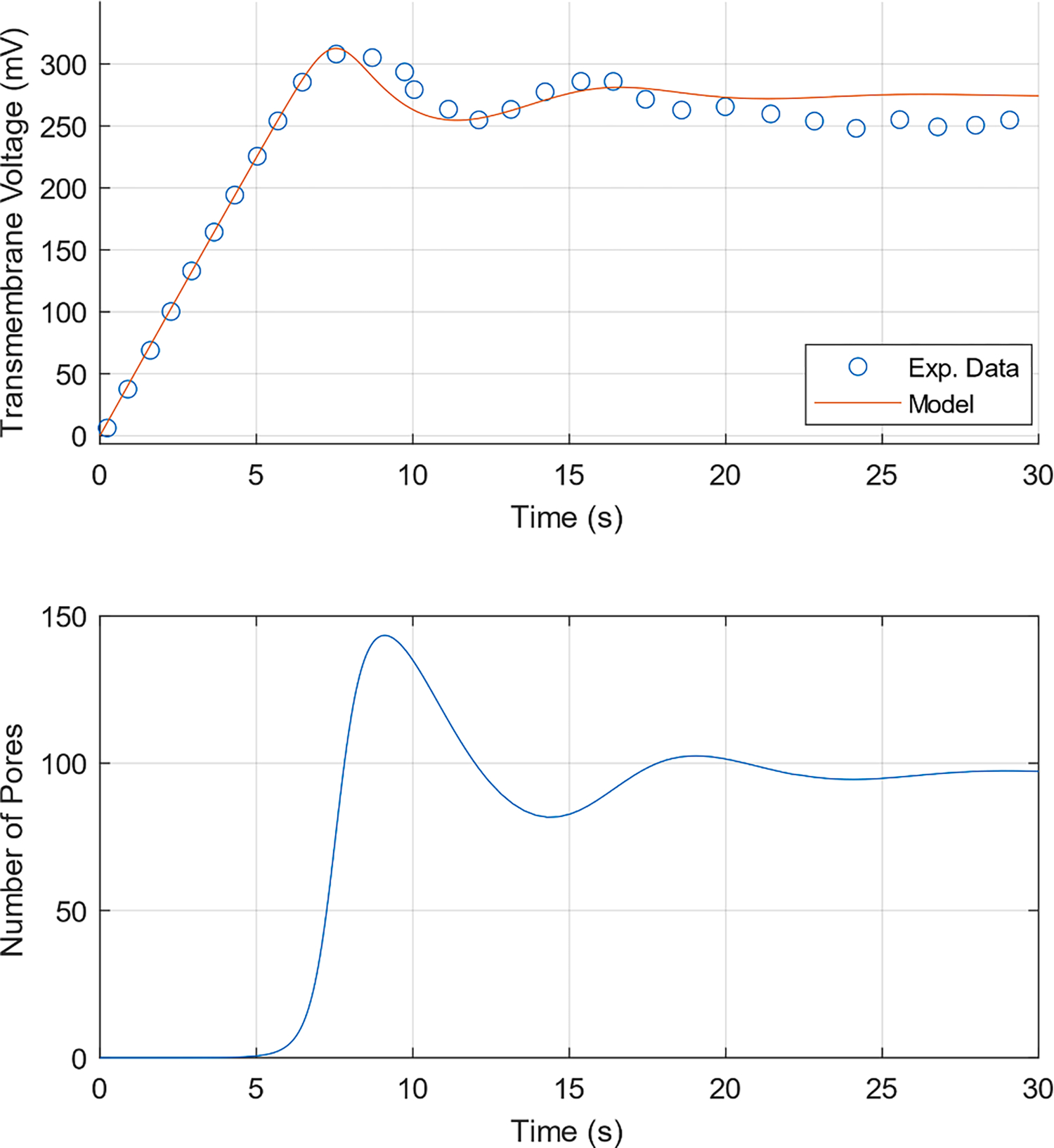
(Smoluchowski model) Current-Clamp Electroporation (j = 1 mA m−2). (Top) Transmembrane Voltage response and Exp. data from Naumowicz et al. [23] reproduced using the Engauge Digitizer Software [33]. (Bottom) Number of Pores as a function of time.
4. Discussion
Using the Smoluchowski and Langevin models, we have shown two potential mechanisms that can account for the voltage oscillations during current-clamp electroporation. The oscillations are either due to the growth and shrinkage of pores via a negative feedback mechanism involving the transmembrane voltage, or they are due to the opening and closing of pores as the system reaches equilibrium. An important conclusion is that the voltage oscillations are not necessarily due to the presence of a single pore. While it is theoretically possible that a single pore can be created under current-clamp conditions, it cannot simply be assumed on the basis of the presence of voltage oscillations. Meanwhile, the voltage-clamp method has been shown to generate a single pore based on the abruptness and magnitude of conductance transitions [4], and visual observation [3]. Therefore, we recommend using the voltage-clamp method to reliably generate a single pore.
For the case involving a single pore (Fig. 3), we observed damped voltage oscillations similar to the experimental data, but we were not able to achieve a good fit using our model. Interestingly, the pore in Fig. 3 (top) reached an equilibrium radius of 16 nm, which is much larger than the 1 nm pores created under voltage-clamp conditions [4]. If a stable 16 nm pore is in fact generated under current-clamp conditions, this would make it ideal for delivery large molecules like plasmid DNA. We also observed that the system exhibits a Hopf bifurcation. A Hopf bifurcation is a feature of certain dynamical systems characterized by a sudden change in its qualitative behavior and the appearance of oscillations. In particular, it occurs when, as a parameter value is smoothly changed, a pair of complex conjugate eigenvalues cross the imaginary axis of the complex plane, resulting in the appearance of an elliptical limit cycle in phase space [34]. However, no continuously oscillating waveform has been reported in the experimental data [23]. Instead, we observe that the voltage oscillations are always damped as the transmembrane voltage reaches a steady-state value. This is another indication that more than a single pore is created under current-clamp conditions. For example, in Figs. 2 and 4, the increase in pore number at the minimum energy radius rm lowers the transmembrane voltage, but a subsequent increase in transmembrane voltage is prevented because the pores cannot shrink or reseal due to the high pore destruction energy barrier (Wd).
We have shown, in the case of low pore number, that the Smoluchowski model produces an artificial smoothing due to the continuous nature of the pore density n(r, t). As a result, the analogous Langevin model we have presented here produces better qualitative agreement with the experimental data. In Fig. 2 of Naumowicz et al. [23], one can observe two characteristic frequencies of voltage oscillations. The high magnitude, low frequency oscillations are observed in both the Smoluchowski and Langevin simulations, but the low magnitude, high frequency oscillations are only seen in the Langevin simulations (Fig. 5). If our model is correct, the low magnitude, high frequency oscillations are due to stochastic pore fluctuations while the high magnitude, low frequency oscillations are due to either a negative feedback mechanism, or a mechanism involving pore opening and closing.
To determine which of the two mechanisms is responsible, the bilayers can be imaged using optical single channel recordings. For the pore opening and closing mechanism, the local energy minimum stays within the range rm = [1 nm 1.1 nm] throughout the simualtion, meaning the most pores observed should have similar radii. According to the conductance model, a pore of raidus 1 nm should have a conductance of 411 pS, which is consistent with the mean pore conductance in Melikov et al. [4]. In contrast, the average pore size is variable for the negative feedback mechanism (Fig. 5), meaning that pores of different sizes should be observed.
Another important property of pores is their mean lifetime or resealing time. The pore resealing time constant is given by [14,16]
| (20) |
Since the steric repulsion energy and edge energy dominate the pore energy landscape near , the corresponding parameters largely determine the value of the pore destruction energy barrier . Many different combinations of the parameters can produce the same value for . Therefore, although we cannot be certain about the values of the parameters , we can be somewhat confident about the value of . Using Eq. (20), we computed a value of at and at 0.3 V for the simulation in Fig. 6. These values are similar to pore lifetimes measured experimentally using planar lipid bilayers [3,4]. Note that electropore lifetimes reported in molecular dynamics simulations and experiments with GUVs are in the nanoseconds range [35,36], while cells remain permeable for minutes [36].
Note that the parameters (a, β, D, γ, B, b) largely depend on membrane composition (in this case a 3:7 M ratio of phosphatidylcholine and cholesterol [23]). Different membranes will likely require different parameter values. It should also be emphasized that the two parameter sets we have chosen here are not necessarily the only ones which produce a good fit with the data, and a better fit could have been achieved by doing an extensive parametric search. However, such a globally optimal fit would likely not give any more useful information, and it is not clear if the corresponding optimal parameters would be any closer to the “true” parameters than the ones we have chosen. For example, consider the value for the diffusion coefficient we have chosen for the simulation in Figs. 2–5 (D = 10−18). It was necessary to pick such a low value to slow down the pore growth rate and properly fit the data. It is possible that the “true” value is much higher, but using such values produces a poor fit with the data because of limitations in the model. Other authors have introduced more sophisticated pore growth models which involve viscous and viscoelastic effects [37,38]. It may be necessary to use such models in the future to uncover the “true” parameter values.
Supplementary Material
Acknowledgements
This work was supported by the National Institutes of Health [grants HL148825, DK120680, HL148695, and HL153988]; and the Cystic Fibrosis Foundation [grant DEAN20XX0].
Footnotes
Declaration of Competing Interest
The authors declare the following financial interests/personal relationships which may be considered as potential competing interests: David A. Dean reports financial support was provided by National Institutes of Health. David A. Dean reports a relationship with OncoSec Medical Incorporated that includes: consulting or advisory.
Appendix A. Supplementary material
Supplementary data to this article can be found online at https://doi.org/10.1016/j.bioelechem.2022.108162.
References
- [1].Kotnik T, Rems L, Tarek M, Miklavčič D, Membrane electroporation and electropermeabilization: mechanisms and models, Annu. Rev. Biophys. 48 (1) (2019) 63–91. [DOI] [PubMed] [Google Scholar]
- [2].Neu WK, Neu JC, Theory of electroporation, in: Efimov IR, Kroll MW, Tchou PJ (Eds.), Cardiac Bioelectric Therapy, Springer US, Boston, MA, 2009, pp. 133–161, 10.1007/978-0-387-79403-7_7. [DOI] [Google Scholar]
- [3].Sengel JT, Wallace MI, Imaging the dynamics of individual electropores, Proc. Natl. Acad. Sci. 113 (19) (2016) 5281–5286. [DOI] [PMC free article] [PubMed] [Google Scholar]
- [4].Melikov KC, Frolov VA, Shcherbakov A, Samsonov AV, Chizmadzhev YA, Chernomordik LV, Voltage-induced nonconductive pre-pores and metastable single pores in unmodified planar lipid bilayer, Biophys. J. 80 (4) (2001) 1829–1836. [DOI] [PMC free article] [PubMed] [Google Scholar]
- [5].Canatella PJ, Karr JF, Petros JA, Prausnitz MR, Quantitative study of electroporation-mediated molecular uptake and cell viability, Biophys. J. 80 (2) (2001) 755–764. [DOI] [PMC free article] [PubMed] [Google Scholar]
- [6].Puc M, Kotnik T, Mir LM, Miklavčič D, Quantitative model of small molecules uptake after in vitro cell electropermeabilization, Bioelectrochemistry 60 (1–2) (2003) 1–10. [DOI] [PubMed] [Google Scholar]
- [7].Sukharev S, Klenchin V, Serov S, Chernomordik L, YuA C, Electroporation and electrophoretic DNA transfer into cells. The effect of DNA interaction with electropores, Biophys. J. 63 (5) (1992) 1320–1327. [DOI] [PMC free article] [PubMed] [Google Scholar]
- [8].Rems L, Applicative use of electroporation models: from the molecular to the tissue level, in: Advances in Biomembranes and Lipid Self-Assembly, Elsevier, 2017, pp. 1–50. [Google Scholar]
- [9].Akimov SA, Volynsky PE, Galimzyanov TR, Kuzmin PI, Pavlov KV, Batishchev OV, Pore formation in lipid membrane I: Continuous reversible trajectory from intact bilayer through hydrophobic defect to transversal pore, Sci. Rep. 7 (1) (2017) 1–20. [DOI] [PMC free article] [PubMed] [Google Scholar]
- [10].Ziegler MJ, Vernier PT, Interface water dynamics and porating electric fields for phospholipid bilayers, J. Phys. Chem. B 112 (43) (2008) 13588–13596. [DOI] [PubMed] [Google Scholar]
- [11].Vasilkoski Z, Esser AT, Gowrishankar T, Weaver JC, Membrane electroporation: The absolute rate equation and nanosecond time scale pore creation, Phys. Rev. E 74 (2) (2006), 021904. [DOI] [PubMed] [Google Scholar]
- [12].Barnett A, Weaver JC, Electroporation: a unified, quantitative theory of reversible electrical breakdown and mechanical rupture in artificial planar bilayer membranes, Bioelectrochem. Bioenerg. 25 (2) (1991) 163–182. [Google Scholar]
- [13].Freeman SA, Wang MA, Weaver JC, Theory of electroporation of planar bilayer membranes: predictions of the aqueous area, change in capacitance, and pore-pore separation, Biophys. J. 67 (1) (1994) 42–56. [DOI] [PMC free article] [PubMed] [Google Scholar]
- [14].Smith KC, A unified model of electroporation and molecular transport, (Ph.D. Thesis) Massachusetts Institute of Technology, 2011. [Google Scholar]
- [15].Smith KC, Weaver JC, Electrodiffusion of molecules in aqueous media: a robust, discretized description for electroporation and other transport phenomena, IEEE Trans. Biomed. Eng. 59 (6) (2011) 1514–1522. [DOI] [PubMed] [Google Scholar]
- [16].Neu JC, Krassowska W, Asymptotic model of electroporation, Phys. Rev. E 59 (3) (1999) 3471–3482. [Google Scholar]
- [17].Krassowska W, Filev PD, Modeling electroporation in a single cell, Biophys. J. 92 (2) (2007) 404–417. [DOI] [PMC free article] [PubMed] [Google Scholar]
- [18].Smith KC, Neu JC, Krassowska W, Model of creation and evolution of stable electropores for DNA delivery, Biophys. J. 86 (5) (2004) 2813–2826. [DOI] [PMC free article] [PubMed] [Google Scholar]
- [19].Kalinowski S, Ibron G, Bryl K, Figaszewski Z, Chronopotentiometric studies of electroporation of bilayer lipid membranes, Biochimica et Biophysica Acta (BBA)-Biomembranes 1369 (2) (1998) 204–212. [DOI] [PubMed] [Google Scholar]
- [20].Koronkiewicz S, Kalinowski S, Influence of cholesterol on electroporation of bilayer lipid membranes: chronopotentiometric studies, Biochimica et Biophysica Acta (BBA)-Biomembranes 1661 (2) (2004) 196–203. [DOI] [PubMed] [Google Scholar]
- [21].Naumowicz M, Figaszewski ZA, Chronopotentiometric technique as a method for electrical characterization of bilayer lipid membranes, J. Membr. Biol. 240 (1) (2011) 47–53. [DOI] [PubMed] [Google Scholar]
- [22].Naumowicz M, Petelska AD, Figaszewski ZA, Chronopotentiometric studies of phosphatidylcholine bilayers modified by ergosterol, Steroids 76 (10–11) (2011) 967–973. [DOI] [PubMed] [Google Scholar]
- [23].Naumowicz M, Figaszewski ZA, Pore formation in lipid bilayer membranes made of phosphatidylcholine and cholesterol followed by means of constant current, Cell Biochem. Biophys. 66 (1) (2013) 109–119. [DOI] [PMC free article] [PubMed] [Google Scholar]
- [24].Kramar P, Miklavčič D, Kotulska M, Lebar AM, Voltage-and current-clamp methods for determination of planar lipid bilayer properties, in: Advances in Planar Lipid Bilayers and Liposomes, Elsevier, 2010, pp. 29–69. [Google Scholar]
- [25].Naumowicz M, Figaszewski ZA, Chronopotentiometric investigation of the influence of cholesterol and ionic strength on lipid bilayer’s physicochemical properties, J. Electrochem. Soc. 160 (3) (2013) H166–H172. [Google Scholar]
- [26].Abidor IG, Arakelyan VB, Chernomordik LV, Chizmadzhev YA, Pastushenko VF, Tarasevich MP, Electric breakdown of bilayer lipid membranes: I. The main experimental facts and their qualitative discussion, J. Electroanal. Chem. Interfacial Electrochem. 104 (1979) 37–52. [Google Scholar]
- [27].Neu JC, Smith KC, Krassowska W, Electrical energy required to form large conducting pores, Bioelectrochemistry 60 (1–2) (2003) 107–114. [DOI] [PubMed] [Google Scholar]
- [28].Neu JC, Krassowska W, Modeling postshock evolution of large electropores, Phys. Rev. E 67 (2) (2003), 021915. [DOI] [PubMed] [Google Scholar]
- [29].Sperelakis N, Origin of resting membrane potentials, in: Cell Physiology Source Book, Elsevier, 2001, pp. 219–236. [Google Scholar]
- [30].Chernomordik LV, Sukharev SI, Popov SV, Pastushenko VF, Sokirko AV, Abidor IG, Chizmadzhev YA, The electrical breakdown of cell and lipid membranes: the similarity of phenomenologies, Biochimica et Biophysica Acta (BBA)-Biomembranes 902 (3) (1987) 360–373. [DOI] [PubMed] [Google Scholar]
- [31].Renkin EM, Filtration, diffusion, and molecular sieving through porous cellulose membranes, J. General Physiol. 38 (2) (1954) 225. [PMC free article] [PubMed] [Google Scholar]
- [32].Schulten K, Chapter 4: Smoluchowski Diffusion Equation, in: Non-Equilibrium Statistical Mechanics, ed, 2003. [Google Scholar]
- [33].Mitchell M, Muftakhidinov B, Winchen T, et al. , Engauge Digitizer Software. http://markummitchell.github.io/engauge-digitizer. [Google Scholar]
- [34].Strogatz SH, Nonlinear Dynamics and Chaos: with Applications to Physics, Biology, Chemistry, and Engineering, CRC Press, 2018. [Google Scholar]
- [35].Levine ZA, Vernier PT, Life cycle of an electropore: field-dependent and field-independent steps in pore creation and annihilation, J. Membr. Biol. 236 (1) (2010) 27–36. [DOI] [PubMed] [Google Scholar]
- [36].Sözer EB, Haldar S, Blank PS, Castellani F, Vernier PT, Zimmerberg J, Dye transport through bilayers agrees with lipid electropore molecular dynamics, Biophys. J. 119 (9) (2020) 1724–1734. [DOI] [PMC free article] [PubMed] [Google Scholar]
- [37].Kroeger JH, Vernon D, Grant M, Curvature-driven pore growth in charged membranes during charge-pulse and voltage-clamp experiments, Biophys. J. 96 (3) (2009) 907–916. [DOI] [PMC free article] [PubMed] [Google Scholar]
- [38].Sung W, Park P, Dynamics of pore growth in membranes and membrane stability, Biophys. J. 73 (4) (1997) 1797–1804. [DOI] [PMC free article] [PubMed] [Google Scholar]
Associated Data
This section collects any data citations, data availability statements, or supplementary materials included in this article.