

Abstract
Assessing species’ extinction risk is vital to setting conservation priorities. However, assessment endeavors, such as those used to produce the IUCN Red List of Threatened Species, have significant gaps in taxonomic coverage. Automated assessment (AA) methods are gaining popularity to fill these gaps. Choices made in developing, using, and reporting results of AA methods could hinder their successful adoption or lead to poor allocation of conservation resources. We explored how choice of data cleaning type and level, taxonomic group, training sample, and automation method affect performance of threat status predictions for plant species. We used occurrences from the Global Biodiversity Information Facility (GBIF) to generate assessments for species in 3 taxonomic groups based on 6 different occurrence‐based AA methods. We measured each method's performance and coverage following increasingly stringent occurrence cleaning. Automatically cleaned data from GBIF performed comparably to occurrence records cleaned manually by experts. However, all types of data cleaning limited the coverage of AAs. Overall, machine‐learning‐based methods performed well across taxa, even with minimal data cleaning. Results suggest a machine‐learning‐based method applied to minimally cleaned data offers the best compromise between performance and species coverage. However, optimal data cleaning, training sample, and automation methods depend on the study group, intended applications, and expertise.
Keywords: automation, biodiversity conservation, IUCN Red List, machine learning, aprendizaje automático, automatización, conservación de la biodiversidad, Lista Roja UICN
Resumen
La valoración del riesgo de extinción de las especies es vital para el establecimiento de prioridades de conservación. Sin embargo, los esfuerzos de valoración, como los que se usan para generar la Lista Roja de Especies Amenazadas de la UICN, tienen brechas importantes en la cobertura taxonómica. Los métodos de valoración automatizada (VA) están ganando popularidad como reductores de estas brechas. Las elecciones realizadas en el desarrollo, uso y reporte de resultados de los métodos de VA podrían obstaculizar su adopción exitosa o derivar en una asignación deficiente de recursos para la conservación. Exploramos cómo la selección del tipo de limpieza de datos y el nivel, grupo taxonómico, muestra de entrenamiento y el método de automatización afectan el desempeño de las predicciones del estado de amenaza de las especies de plantas. Usamos los registros de la Global Biodiversity Information Facility (GBIF) para generar las valoraciones de las especies de tres grupos taxonómicos con base en seis métodos diferentes de VA basados en la presencia de las especies. Medimos el desempeño de cada método y cobertura después de una limpieza de presencia cada vez más estricta. La información de la GBIF limpiada automáticamente tuvo un desempeño comparable con los registros de presencia limpiados manualmente por expertos. Sin embargo, todos los tipos de limpieza de datos limitaron la cobertura de las valoraciones automatizadas. En general, los métodos basados en el aprendizaje automático tuvieron un buen desempeño en todos los taxones, incluso con una limpieza mínima de datos. Los resultados sugieren que un método basado en el aprendizaje automático aplicado a información con la mínima limpieza ofrece el mejor equilibrio entre el desempeño y la cobertura de la especie. A pesar de esto, la limpieza óptima de datos, la muestra de entrenamiento y los métodos de automatización dependen del grupo de estudio, las aplicaciones deseadas y la experiencia.
INTRODUCTION
Evaluating species extinction risk is critical in acting to protect biodiversity. The International Union for Conservation of Nature (IUCN) Red List of Threatened Species (hereafter RL), the internationally accepted standard for species’ global extinction risk assessments, covers some groups comprehensively (e.g., birds) but only ∼15% of vascular plant species (IUCN, 2021a). Gaps in extinction risk knowledge may lead to inappropriate conservation resource allocation. Automated assessments (AAs) based on occurrence records from natural history collections can help close assessment gaps (Nic Lughadha et al., 2020). Growing recognition of the imperative to accelerate extinction risk assessments (Bachman et al., 2019), advances in digitization of natural history collections (Paton et al., 2020), and widening availability of biodiversity data have stimulated AA method development. However, systematic exploration of methods is necessary for their effective application.
Assessing species for the RL involves gathering data and calculating metrics to apply 1 or more of 5 quantitative criteria (IUCN, 2012) related to population size reduction (criterion A), geographic range size and fragmentation (criterion B), small and declining population size (criterion C), very small and restricted populations (criterion D), and quantitative analysis (criterion E).
AA methods can be organized into 2 approaches, those based on calculating parameters to directly apply RL criteria and those predicting RL categories based on selected correlates of extinction risk. A recent review terms these approaches criteria explicit and category predictive, respectively (Cazalis et al., 2022). Researchers have developed methods for different taxa that calculate parameters and predictors from information, including species ranges (Bird et al., 2012), occurrence records (Dauby et al., 2017; Zizka, Silvestro, et al., 2020), known threats and human pressure (Di Marco et al., 2018; Greenville et al., 2021), and species characteristics (Pelletier et al., 2018; Safi & Pettorelli, 2010). Although most methods use parameters or predictors relating to range size (criterion B), population decline (criterion A), or both, methods exist to apply all criteria except E (Santini et al., 2019; Visconti et al., 2016).
For plants occurrence records in natural history collections and digital resources represent the most readily available distribution data (Nic Lughadha, Walker, et al., 2019). Therefore, most AA methods developed for plants use parameters or predictors calculated from occurrence records (Cazalis et al., 2022). These are mostly associated with range size (criterion B), although some include measures or correlates of changes in population size (criterion A; Stévart et al., 2019; Zizka et al., 2022).
Accessible tools employing AA methods include the criteria‐explicit approaches rCAT (Moat, 2020), rapidLC (Bachman et al., 2020), and ConR (Dauby et al., 2017) and category‐predictive approach IUCNN (Zizka et al., 2022). Automated methods have been applied to large data sets in the preliminary assessment of 22,036 tropical African plants (Stévart et al., 2019), 13,910 orchid species (Zizka, Silvestro, et al., 2020), and over 150,000 land plants (Pelletier et al., 2018).
Authors of these studies acknowledge the limitations in their approaches, but suggest their new methods can inform conservation prioritization. For example, Stévart et al. (2019) propose areas of “high conservation value,” and Pelletier et al. (2018) propose global “geographic regions with the highest need of conservation efforts.” However, complete information required for potential users to evaluate method performance and the resulting conservation priorities is not consistently reported (Walker et al., 2020). Given the high‐stakes applications of AA methods, thorough consideration of their benefits and limitations seems prudent and practitioners wishing to adopt automated methods need clear guidelines about method choice and appropriate use.
We considered 4 questions central to successful use of AA methods: How clear must occurrence data be? Which sample of assessments is most effective for training and evaluating AA methods? Must individual IUCN criteria be considered? And, when should one AA method be used over another?
Quality problems affecting occurrence records in online databases are well documented (Meyer et al., 2016; Panter et al., 2020; Paton et al., 2020). Species occurrences are, therefore, manually checked during RL assessments, requiring significant time investment. Occurrence‐based AA methods typically use automated cleaning on digitally available records to save time, but overly strict cleaning could limit benefits of AAs. Automated cleaning is more important for criteria‐explicit than category‐predictive methods (Zizka, Silvestro, et al., 2020), but effects vary across taxa (Zizka, Antunes Carvalho, et al., 2020).
Manual RL assessments are needed to measure AA method performance and train machine‐learning‐based methods. To maximize sample size, analyses usually use all assessed species in a study group. However, given historically nonsystematic choices of species for assessment (Nic Lughadha et al., 2020), assessed species may not represent group diversity. Furthermore, imbalances in species numbers assessed across RL categories present problems for machine‐learning models. Previous studies addressed these issues using a random subset of species assessed for the Sampled Red List Index (SRLI) (Zizka, Silvestro, et al., 2020) or correcting imbalances through downsampling (Pelletier et al., 2018).
Most plant assessments apply criterion B (Nic Lughadha, Walker, et al., 2019); species distributions are calculated from occurrence records. Similarly, most occurrence‐based AA methods for plants use parameters related to criterion B. It remains unclear whether occurrence‐based AA methods can predict the status of species assessed under non‐B criteria equally well.
Both criteria‐explicit and category‐predictive methods can predict extinction risk from manual RL assessments with high accuracy, but each offers distinct advantages. Criteria‐explicit methods facilitate interpretation and troubleshooting, whereas machine‐learning methods may be more robust to unclean data. The desired balance between predictive accuracy, ease of use, and interpretability may depend on available data, species group, and intended users.
We systematically investigated choice of type and level of data cleaning, assessment sample, and AA method by applying 6 different occurrence‐based methods to generate preliminary assessments for 3 groups of flowering plants. We compared performance of these methods on digitally available occurrence data with different levels of automated cleaning and manually cleaned occurrences. We examined how choices concerning training data and downsampling affect performance. We developed evidence‐based recommendations for use of AA methods and highlight important unanswered questions.
METHODS
Data compilation and cleaning
We chose 3 taxonomically and geographically distinct species plant groups with different collection histories to evaluate effects and performance of choices in AA methods: Myrcia, Orchidaceae, and Leguminosae.
The Neotropical genus Myrcia (∼750 spp., family Myrtaceae) is taxonomically complex; thus, species records in digital resources, like the Global Biodiversity Information Facility (GBIF), often contain substantial identification errors. After decades of taxonomic impediment, molecular analyses and collaborative systematics are facilitating monography. Access to a monographer's specimen database allowed comparison of manual and automatic data collection and cleaning.
Only 5% of the family Orchidaceae (∼30,000 spp., orchids) have been assessed for the RL. Rapid preliminary assessments could help focus resources on potentially threatened species. Furthermore, previous AAs of orchids (Zizka, Silvestro, et al., 2020) allow direct comparison of results.
Leguminosae (∼22,000 spp., legumes) is another large family but is relatively well understood taxonomically and well documented (e.g., Lewis et al., 2005). Legumes are well represented in the SRLI, enabling comparison of the effects of training and evaluation of AA methods on a random sample against all assessed legumes on the RL.
We obtained checklists of accepted species names for these groups from the World Checklist of Vascular Plants (WCVP) (Govaerts et al., 2021).
Species assessments
We downloaded published assessments for the 3 species groups from the RL (IUCN, 2021b). We matched assessment names to WCVP and updated accepted names of assessments matched to homotypic synonyms. We removed assessments matched to nonhomotypic synonyms, unmatchable assessments, and those that matched species outside our accepted species lists.
Occurrence record sources and cleaning
We downloaded occurrence records from GBIF for the families to which our groups belonged and matched taxon names of these occurrences to WCVP taxonomy (Appendix S1). For Myrcia, we retrieved expert‐verified occurrence records from a monographer's database of Myrcia s.l. (E. Lucas provided data).
We passed each set of occurrences through automated cleaning steps with 2 approaches: filtering records lacking preserved voucher specimens (hereafter unvouchered) or representing duplicates and removal of records based on possibly erroneous coordinates. We applied filters to test whether removing unvouchered occurrences or removing duplicated occurrences affected extinction risk prediction. The combination of these filters led to 4 different levels of filter‐based cleaning (Table 1).
TABLE 1.
Filtering and coordinate cleaning steps applied to occurrence records downloaded from the Global Biodiversity Information Facility and used in the automated assessment of plant species*
| Step | Description |
|---|---|
| 1 | No filtering of occurrence records |
| 2 | Keep only vouchered records (those based on preserved specimens) |
| 3 | Keep 1 of every record at exactly the same coordinates for each species |
| 4 | Apply filter steps 2 and 3 |
| A | No geography‐based cleaning |
| B | Remove occurrence records with coordinates (0, 0) |
| C | Remove occurrence records in the sea, at equal longitude and latitude, at country centroids, and at identified institutions |
| D | Remove occurrence records outside each species’ native range as listed in Plants of the World Online |
Filtering steps were applied separately. Coordinate cleaning steps were applied consecutively (i.e., step C was applied to a data set already cleaned in step B).
We chose coordinate‐cleaning steps based on other AA methods studies (e.g., Bachman et al., 2020), 2 of which (B and C) are implemented in the CoordinateCleaner package (Zizka et al., 2019). We applied each step sequentially (Table 1). We passed all GBIF occurrence data sets through all permutations of these filtering and cleaning steps, generating 16 occurrence records sets for each species group and an additional set of occurrences from the Myrcia monographic database.
Method training and evaluation
We generated extinction risk predictions for species groups from 6 different AA methods (Table 2) with sets of parameters and predictors calculated from the occurrences in our cleaned data sets. We calculated these predictors (Appendix S10) for each species in the data set (Appendix S1).
TABLE 2.
Description of the automated assessment methods compared for performance at predicting extinction risk of plant species and ease of use and interpretation
| Method a | Type | Description | Predictors b | Interpretation |
|---|---|---|---|---|
| EOO (extent of occurrence) threshold | Criteria explicit | IUCN criterion B threshold for EOO of threatened species (EOO < 20,000 km2) | EOO | – |
| ConR | Criteria explicit | IUCN criterion B thresholds on EOO, area of occupancy (AOO), and number of threat‐defined locations as calculated with ConR package | EOO, AOO, number of locations | – |
| Decision stump | Category predictive (machine learning based) | Decision tree with a single split on species’ EOO; requires more expertise than IUCN threshold but is still readily interpretable | EOO | Inspecting the learned classification boundary |
| Decision tree | Category predictive (machine learning based) | Decision tree model limited to maximum of 5 splits and using predictors, including EOO and measures of species’ environment and exposure to threats; more splits and predictors than decision stump make this method harder to use and understand | EOO, latitude of range centroid, human population density (HPD), human footprint index (HFI), forest loss, elevation, precipitation in the driest quarter, average annual temperature | Visualizing the splits in the decision tree as a flow chart |
| Random forest | Category predictive (machine learning based) | Random forest model with same set of predictors as decision tree; method harder to interpret and use but performed well in previous studies predicting extinction risk (Darrah et al., 2017; Nic Lughadha, Walker, et al., 2019; Pelletier et al., 2018) | As above | Calculating SHapely Additive exPlanations (SHAPs; Lundberg & Lee, 2017) to give individual contribution of each predictor to each prediction |
| IUCNN | Category predictive (machine learning based) | Densely connected neural network built and trained as implemented by the IUCNN package (Zizka et al., 2022) and using the same set of predictors as decision tree; harder to interpret, like the random forest, but performed well in a previous study (Zizka et al., 2022) | As above | As above |
We compared 2 criteria‐explicit methods: one that applied the IUCN threshold for extent of occurrence (EOO) and the other that applied IUCN thresholds for EOO, area of occupancy, and number of locations calculated by ConR. The other 4 methods investigated were machine‐learning‐based category‐predictive methods with some subset of 8 predictors (EOO, latitude of range centroid, maximum elevation, human population density (HPD), human footprint, forest loss, mean annual temperature, and precipitation in the driest quarter): a decision stump with EOO as sole predictor, a decision tree limited to 5 splits on all predictors, a random forest model with all predictors, and a densely connected neural network (following IUCNN's implementation) with all predictors.
The EOO threshold method, decision stump, decision tree, and random forest provide a progression from simple to use and interpret to a black‐box machine‐learning method. The ConR and IUCNN provide accessible implementations for users.
We grouped species threat categories to reduce imbalance between classes. We grouped critically endangered, endangered, and vulnerable categories as threatened (IUCN, 2012) and near threatened and least concern categories as nonthreatened. We treated data‐deficient species as unassessed and excluded extinct and extinct in the wild species.
We used 10 repeats of 5‐fold cross‐validation to train and evaluate our decision stump, decision tree, random forest, and neural network models. We tuned the hyperparameters of the random forest and neural network models with nested cross‐validation (Appendix S1). We used 50 bootstrap resamples of species with assessments to evaluate our criteria‐explicit methods.
We measured the accuracy of all methods and their sensitivity (proportion of threatened species correctly identified), specificity (proportion of nonthreatened species identified correctly), and true skill statistic (TSS), which balances the sensitivity and specificity (Appendix S1). We also calculated the coverage of each cleaned occurrence data set as the proportion of each species group for which a prediction could be made (i.e., the proportion of species with at least 1 occurrence record).
Analyses
We compared the performance of the 6 AA methods across our 3 taxonomic groups for each of the 16 cleaned occurrence data sets. For Myrcia, we compared performance after the automated cleaning steps with performance on occurrences from the monographic database.
We examined 3 aspects of the training and evaluation sample: representativeness, size, and balance of threatened to nonthreatened species. We addressed representativeness by comparing our AA methods’ performance on all assessed legumes with performance on legumes assessed for SRLI, a sample designed to represent legume taxonomic and geographic diversity. We compared performance of all machine‐learning‐based methods evaluated by taxonomic block cross‐validation to estimate their performance on as‐yet unassessed groups of plants (Appendix S1).
We evaluated sample‐size effects when training our 3 machine‐learning‐based AA methods by splitting our data sets into 5 cross‐validation folds, training our models on subsamples of training data, and measuring subsequent performance on validation sets. We increased subsample size from 100 to 600 species in increments of 100. We also evaluated each model's performance with a training set combining all 3 data sets. We assessed the effect of sample balance on our 3 machine‐learning‐based AA methods by downsampling training sets to balance numbers of threatened and nonthreatened species, following Pelletier et al. (2018).
The IUCN RL assessments list the criteria on which a species’ threaten status is based. We compared the ability of each method to identify threatened species (sensitivity) with assessments citing each criterion (A–D). No assessments in our data set cited criterion E.
Along with AA method performance, we compared the interpretability of the machine‐learning‐based methods with approaches outlined in Table 2. For the black‐box machine‐learning methods, random forest, and IUCNN, we calculated Shapley additive explanations (SHAP)—a method that applies game theory to quantify the contribution of each predictor to an individual prediction (Lundberg & Lee, 2017). We limited this comparison to models trained on the orchid data set with minimally cleaned data (filtering step 1 and coordinate cleaning step A) because orchids are more challenging to predict accurately than other plant groups (Nic Lughadha, Walker, et al., 2019).
All analyses were performed in R (R Core Team, 2020), and the packages we used are detailed in Appendix S1. The code used in our analyses is archived on Zenodo (https://doi.org/10.5281/zenodo.4900043 and https://doi.org/10.5281/zenodo.6398923). All analysis outputs are archived on Zenodo (https://doi.org/10.5281/zenodo.4899924). The occurrence record data sets we used can be downloaded from GBIF (Myrcia: https://doi.org/10.15468/dl.netuzf, legumes: https://doi.org/10.15468/dl.emrcnf, orchids: https://doi.org/10.15468/dl.47vwfd).
RESULTS
Effects of data cleaning
After name‐matching GBIF occurrences with coordinates (step 1A), the Myrcia data set was smallest, with 60,134 records representing 666 (87.5%) accepted species, and was followed by orchids, with 4,497,935 records for 18,859 (61.8%) accepted species, and legumes, with 16,307,895 records for 18,735 (84.0%) accepted species.
Most Myrcia records were vouchered (93.5%); corresponding proportions were much smaller for the orchid (14.5%) and legume (15.3%) data sets. Therefore, filtering step 2 (removing unvouchered records) removed most orchid and legume records but few Myrcia records. Filtering step 3 (removing records at duplicated coordinates) reduced the Myrcia data set to 35,330 unique occurrences (58.8%), orchids to 2,109,409 (46.9%), and legumes to 9,655,750 (59.2%).
The coordinate‐cleaning steps removed fewer records than filtering steps. Coordinate‐cleaning step C removed the most records from orchids (7.0%), whereas step D removed most from Myrcia (7.4%) and legumes (13.5%). Applying all filtering and coordinate‐cleaning steps removed 48.8% of Myrcia, 90.8% of legume, and 91.1% of orchid occurrences, respectively. The Myrcia database comprised 10,724 occurrences, less than half the number in the automatically cleaned data set.
Applying all filtering and cleaning steps reduced prediction coverage (Appendix S2) to 619 of 761 Myrcia species (81.3%), 17,752 of 22,307 legumes (79.6%), and 17,045 of 30,530 orchids (55.8%). Concurrently, numbers of species with non‐DD assessments (i.e., assessments with any other category from least concern to critically endangered) available to train and evaluate the AA methods were reduced to 339 of 358 Myrcia species, 4097 of 4323 legumes (831 assessed for SRLI), and 1201 of 1510 orchids. The monographic database covered 545 Myrcia species (71.6% of accepted Myrcia species), 309 of which were available to train and evaluate AA methods.
All methods performed well across every filtering and cleaning step; TSS was consistently above 0.25 (Appendix S3). Performance improvement was large for the EOO threshold method from coordinate‐cleaning steps A–D, except for Orchids (Figure 1). Mean TSS increased from 0.54 to 0.61 for Myrcia, 0.40 to 0.58 for SRLI legumes, and 0.52 to 0.60 for all legumes. Filtering steps 2, 3, and 4 had negligible impacts on performance.
FIGURE 1.
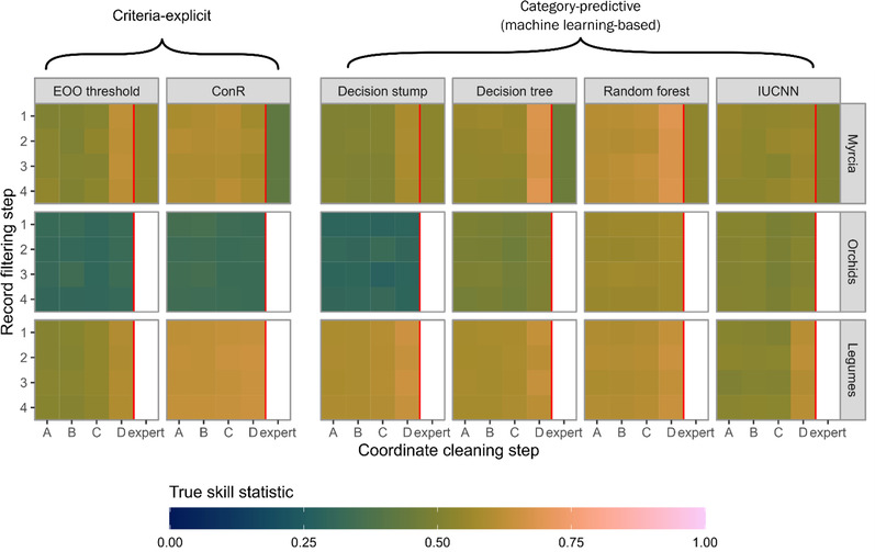
Performance of automated assessment methods on data sets of Myrcia, orchid, and legume species after automated occurrence record filtering and coordinate cleaning (EOO, extent of occurrence; IUCN, International Union for Conservation of Nature). Results for Myrcia include a data set of expert‐cleaned occurrences (expert). Filtering and cleaning steps are described in Table 1.
Performance was slightly poorer on the Myrcia monographic database than on GBIF data with full coordinate cleaning. Random forest models performed worse on data from the monographic database (TSS = 0.53) than on minimally cleaned GBIF data (0.60).
Automated cleaning improved the performance of most methods on Myrcia and legumes but resulted in minimal improvement for orchids. However, IUCNN showed no clear improvement on Myrcia with cleaning, whereas automated cleaning had little impact on the performance of ConR for all data sets.
Most effective sample assessments for training and evaluating AA methods
A small proportion of SRLI legume assessments were threatened (11.8%). Although all 4 machine‐learning‐based methods showed accuracy above 80% on this sample (Figure 2a), models trained on the SRLI assessments had low sensitivity (decision stump: 0.12; decision tree: 0.32; random forest: 0.28; IUCNN: 0.04). Downsampling improved sensitivity for all machine‐learning‐based models trained on SRLI assessments (decision stump: 0.93; decision tree: 0.76; random forest: 0.84; IUCNN: 0.67) (Figure 2a) but caused little to no improvement for methods trained on all legumes, Myrcia, or orchid species (Appendix S4) that had lower class imbalance (27.8%, 46.1%, and 52.5% threatened, respectively).
FIGURE 2.
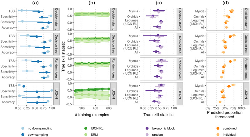
Exploration of sample choice for training and evaluation of automated assessment (AA) methods: (a) effect of downsampling on different performance metrics when AA methods are trained and evaluated on a representative sample of legume species used for the sampled red list index (SRLI), (b) change in machine‐learning‐based AA method performance as the method is trained on successively larger subsets of all legumes assessed for the International Union for Conservation of Nature (IUCN) Red List and those used for the SRLI, (c) difference in estimated true skill statistic (TSS) when using taxonomic block cross‐validation and random cross‐validation, and (d) difference in percentage of unassessed species predicted threatened when AA methods are trained and evaluated on individual data sets and on 1 combined data set (bars [a, c, d] and shading [b], 95% confidence interval of the cross‐validated estimates)
Even with downsampling, all AA methods performed worse when trained on SRLI legume assessments than all assessed legumes (Figure 2a; Appendix S4). This difference in TSS persisted regardless of training sample size, especially for the IUCNN method (Figure 2b).
Overall, taxonomic block cross‐validation gave similar estimates of average method performance to random cross‐validation but had higher variance (Figure 2c). Block cross‐validation did, however, give a notably lower estimate of performance for the random forest (block: 0.46; random: 0.58) and IUCNN (block: 0.37; random: 0.52) methods when trained on all species combined.
Training machine‐learning‐based models on all groups combined caused little or no improvement in our evaluation metrics (Appendix S5) but did reduce sensitivity for Myrcia species. This reduction corresponded to a lower predicted level of threat in unassessed Myrcia species when data sets were pooled (Figure 2d).
Consideration of individual IUCN criteria
Over 80% of threatened assessments in our 3 study groups cited criterion B (Appendix S11). Criterion A was next most frequently cited, especially for Myrcia species (23.6% of assessments).
The EOO threshold and ConR methods had lower accuracy in all study groups when predicting threatened species (sensitivity) with assessments citing criterion A (Figure 3), with the largest differences being in Myrcia species (EOO threshold: 7.3% with A, 78.0% without A; ConR: 27.2% with A, 95.7% without A). Random forest and IUCNN methods, however, had negligible drops in performance when identifying threatened Myrcia and legume species assessed under criterion A.
FIGURE 3.
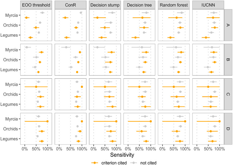
Comparison of the sensitivity (proportion of threatened species correctly identified) of each occurrence‐based automated assessment method for species with assessments citing a particular criterion (EOO, extent of occurrence; IUCN, International Union for Conservation of Nature) (criteria [right‐hand axis]: a, population size reduction; b, geographic range size and fragmentation; c, small and declining population size; d, very small and restricted populations; no species in our datasets were assessed under criterion; e, quantitative analysis, which is not displayed.)
Choice of the appropriate AA method
All AA methods investigated achieved high predictive accuracy, regardless of occurrence record cleaning (Appendix S6). All methods were better at correctly predicting nonthreatened Myrcia and legume species than threatened ones (higher specificity than sensitivity) but were generally as good at predicting threatened orchids as nonthreatened ones. The EOO threshold method showed greatest imbalance across all data sets (Appendix S6) and ConR showed the least. The random forest model consistently scored highest with TSS (Figure 1) followed by ConR, whereas the decision stump, EOO threshold, and IUCNN methods most often scored the lowest.
We compared the interpretability of our machine‐learning models by applying different methods to explore their behavior on the orchid data set (Table 2). The decision stump model learned an average threshold on EOO of 45,522 km2 to identify threatened orchid species, higher than the IUCN threshold of 20,000 km2, but the 95% confidence interval was wide (2851 to 86,179) (Figure 4a).
FIGURE 4.
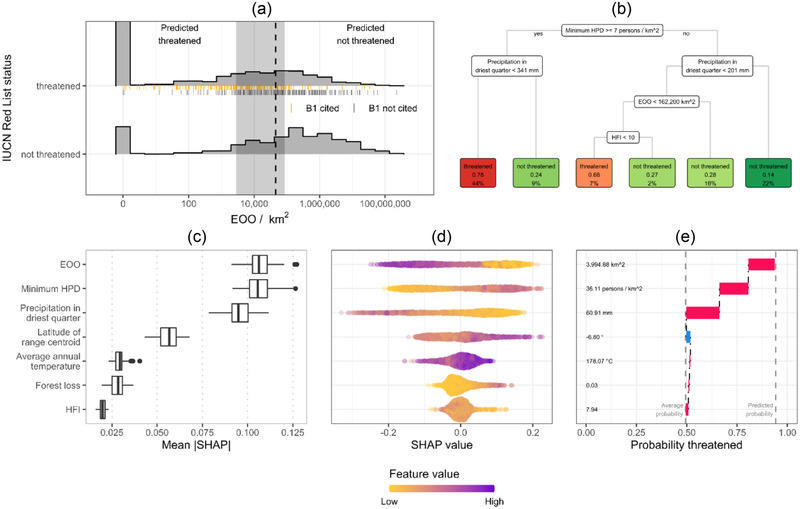
Methods for interpreting machine‐learning‐based automated assessment methods for predicting extinction risk of species. (a) Decision stump model interpreted by inspecting the classification boundary (95% confidence interval [shaded band] estimated by cross‐validation) (lines underbars, assessments citing International Union for Conservation of Nature criterion B1). (b) The decision tree provides a simple flowchart displaying splits in the tree and final decisions as leaves (top number in boxes, classification probability; bottom number in boxes, percentage of species). Shapely additive explanations (SHAPs) are used to interpret behavior of the random forest model. These values estimate the contribution of each predictor in the model to individual predictions and can be aggregated to give (c) the overall importance of each predictor and (d) an indication of how the contribution of each predictor varies with that predictors value. (e) Force plots provide contextual information for a single prediction. All interpretations shown were for models trained on the orchid data set with minimal automated cleaning (step 1A). The individual explanation is for Tridactyle phaeocephala.
The decision tree (Figure 4b) learned to classify most threatened species (44% of species in the training set) based on a minimum HDP >7.2 persons/km2 and driest quarter precipitation <34.1 mm. However, this pathway only classified 78% of these species correctly.
The 3 most important random forest predictors for the orchid data set (Figure 4c) were EOO (mean|SHAP| = 0.107), minimum HPD (mean|SHAP| = 0.106), and precipitation in the driest quarter (mean|SHAP| = 0.096). Ranking of the most important predictors was consistent when calculated by permutation (Appendix S7). For orchid assessments citing criteria A (Appendix S9), the most important predictor changed to minimum HPD (mean|SHAP| = 0.116).
The SHAP‐based partial dependence plot (Figure 4d) revealed our orchid random forest model behaving as expected. More populated areas (higher minimum HPD) increased the predicted probability of threat. In contrast, more precipitation in the driest quarter or larger ranges (higher EOO) reduced the predicted probability of threat.
We examined the contribution of each predictor to a random forest prediction for Tridactyle phaeocephala (Orchidaceae) to illustrate an individual explanation. The SHAP force plot (Figure 4e) indicated that low precipitation in the driest quarter (60.9 mm), small EOO (3995 km2), and relatively high HPD (36.1 persons/km2) elevated the probability of being threatened to 0.94, above the average predicted probability of 0.49. However, the RL category for this species is least concern, despite its low EOO, because no threats have been identified.
We also calculated permutation importance and SHAP values for the IUCNN orchid predictions (Appendices S7 & S8). These calculations showed that the model‐agnostic interpretation methods can also explain the behavior of neural networks. The EOO predictor was less important to the IUCNN orchid predictions, with precipitation in the driest quarter being the most important predictor for permutation importance and SHAP importance.
DISCUSSION
Data cleaning
Well‐documented issues with digitally available occurrences (Meyer et al., 2016; Zizka et al., 2019) suggest that occurrence‐based AA methods should perform better with carefully cleaned data. For example, Panter et al. (2020) report more reliable preliminary assessments with manually cleaned GBIF data. However, this effect is small across different taxa for at least 1 criteria‐explicit method (Zizka, Antunes Carvalho, et al., 2020).
Our results show that, despite these issues, AA methods using automatically cleaned GBIF data give comparable or better performance than hand‐cleaned occurrence data. Although our comparison used a relatively small set (∼200 Myrcia species), the high accuracy reported for other AA methods supports our findings (Nic Lughadha, Walker, et al., 2019; Stévart et al., 2019; Zizka, Silvestro, et al., 2020).
Optimal cleaning levels for criteria‐explicit AA methods vary with study group (Zizka, Antunes Carvalho, et al., 2020). Data cleaning improved EOO threshold method performance for Myrcia and legume, but not orchid species. Zizka, Silvestro, et al. (2020) similarly report ConR accuracy on orchids as unimproved by data cleaning, although our results indicate this may be because ConR is relatively insensitive to automated data cleaning.
Machine‐learning methods were less sensitive to data cleanliness. Scope to use minimally cleaned data is important due to trade‐offs between stringent cleaning and species coverage. Recent large‐scale predictions of plant extinction risk have been affected by such trade‐offs, generating predictions for fewer than half of the species in their target groups (Pelletier et al., 2018; Zizka, Silvestro, et al., 2020). However, some automated cleaning may be necessary for sensible predictions of individual species. For example, occurrence records with clearly erroneous coordinates artificially extended a species’ EOO, whereas removing these occurrences (steps B and C in our analyses) had minimal effect on numbers of species covered by predictions.
Many plant species have few or no digitally available occurrences. These species are mostly rare, range restricted, and likely to be threatened. One potential solution (Darrah et al., 2017) replaces occurrences with coarse‐scale distribution data, available for almost all species (POWO, 2022). However, some predictors used in AA methods may have artificially low variation at this scale, meriting further exploration. Without means of handling species lacking digital occurrence records, one risks ignoring the most threatened species and underestimating the number of threatened species globally.
Most effective sample of assessments for training and evaluating AA methods
Although maximizing training data is often deemed best for machine‐learning‐based AA methods, well‐known gaps and biases in species selected for assessment may lead to poor predictive performance.
Using a sample of species designed to represent the diversity of the study group was not successful. Models trained on all legume assessments outperformed models trained on species assessed for SRLI. This discrepancy remained when models were trained on equal‐sized subsamples of the 2 sets of assessments, suggesting differences in performance were likely due to imbalance between threatened and nonthreatened species in the SRLI.
Downsampling improved overall performance of all machine‐learning‐based models trained on SRLI assessments at small cost to predictive accuracy. However, downsampling made little difference to performance on other data sets with lower imbalance.
Similarly, we saw no benefit to performance when combining taxon‐specific assessments in a single training set. Conversely, we saw a small reduction in ability to identify threatened Myrcia species and a corresponding decrease in the proportion of unassessed Myrcia species predicted as threatened. Methodological choice impacts may not be fully apparent when evaluated on a single taxonomic or geographic group, even one as large as the orchid family. The importance of between‐group variation in method performance is reinforced by the discrepancy we found in estimated performance measured by taxonomic block cross‐validation compared with random cross‐validation. Taxonomic block cross‐validation, where models are trained and evaluated on species from different taxonomic groups, resulted in more variable performance estimates and, in some cases, lower performance. These results suggest machine‐learning‐based methods trained on 1 taxonomic group may not generalize well to other groups.
Consideration of individual IUCN criteria
The AA methods were worst at identifying threatened species assessed under RL criterion A. Reduction in performance was greatest for the EOO threshold and ConR methods, suggesting that criteria‐explicit methods are most sensitive to species assessed under different criteria. Stévart et al. (2019) extended ConR (Dauby et al., 2017) to include estimates of species’ decline to address criterion A but did not report their approach's accuracy on species assessed under this criterion. Our results suggest that machine‐learning‐based methods can achieve good performance across criteria, provided they include appropriate predictors.
Deciding on the appropriate AA method
The random forest model performed best across study groups, regardless of occurrence cleaning. However, fully automated cleaning resulted in even the simplest EOO threshold method matching random forest performance.
Ease of use and understanding are often as important as performance when deciding which method to use. Despite good performance, machine‐learning models, such as random forests and neural networks, require more expertise to apply than criteria‐explicit methods, and their complexity makes it harder to understand individual predictions (Wearn et al., 2019).
When developing new AA methods, key considerations include the intended purpose and user. Most AA methods developed for plants aim to prioritize or inform assessments of unassessed species. The most likely users could be species assessors with little experience with machine learning or scientists employed specifically to apply AA methods. Both ConR and IUCNN are implemented in packages that lower the barrier to their use, but they still require knowledge of a programing language, as all the methods investigated do.
Recent developments have facilitated interpretation of black‐box algorithms, such as random forests and neural networks (Molnar, 2022). We used SHAP (Lundberg & Lee, 2017) to identify the most important predictors, examine how the predicted probability of being threatened depended on each predictor, and diagnose possible deficiencies in predictor choice. However, SHAP involves additional computation, and outputs may not be readily understood by nonexperts.
Perhaps the most significant sources of uncertainty for occurrence‐based AA methods are imprecise or incorrect coordinates and misidentifications in occurrences (Nic Lughadha, Staggemeier, et al., 2019), which cannot be fully addressed by automated cleaning. The goal of quantifying uncertainty for individual extinction risk predictions has yet to be attained (Walker et al., 2020) but may be achieved through Bayesian methods (Hill et al., 2020; Zizka et al., 2022). Such prediction‐specific uncertainty estimates would be invaluable to both threshold and machine‐learning‐based AA methods.
GUIDELINES
The following evidence‐based guidelines can lower barriers to the use and development of AA methods.
Optimal cleaning is, to some degree, dependent on the species group examined, but good performance is possible with automated cleaning of occurrence records. We recommend minimal cleaning, enough to remove obvious errors, in conjunction with a machine‐learning‐based AA method for optimal species coverage. If a criteria‐explicit method is preferred, more stringent automated cleaning is necessary for best performance.
Our results favor using all assessed species, even when well‐designed subsamples are available. Machine‐learning‐based AA methods can make biased predictions when trained on unbalanced samples of assessments, but downsampling can counteract this. Evaluating methods with block cross‐validation and disaggregating performance helps identify when AA methods are performing poorly on subgroups of species.
The AA methods performed better when identifying threatened species assessed under criterion B. Including predictors related to other criteria, such as HPD, helped close this gap for machine‐learning methods in our study. However, the paucity of data relevant to criteria other than B can make this difficult, especially for criteria‐explicit methods.
The most appropriate AA method depends on the availability of resources for data cleaning and expertise to implement the chosen method. However, our results indicated that random forest models perform well across taxonomic groups even with minimally cleaned occurrence data. Methods like SHAP and frameworks like tidymodels can help make them accessible to a wider variety of users. In addition, our study raised further questions presenting possible challenges when using AA methods. Many plant species have few or no digitally available occurrences. This limits applicability of AA methods and risks excluding the most threatened species from assessment pipelines. An AA method must incorporate robust rules to handle these species.
Presenting AA predictions alongside uncertainty estimates would allow better decisions and open new research avenues. Although estimating uncertainty in machine‐learning predictions is possible, there may be more value in quantifying uncertainty from imprecisions in the occurrence data.
Supporting information
Supporting Information
ACKNOWLEDGMENTS
We acknowledge the dedication of Kew's Plant Assessment Unit team who, collaborating with regional and taxon specialists at Kew and worldwide, assessed the extinction risk of many orchids and legumes and most Myrcia species included in our study. The Plant Assessment Unit was a collaboration between IUCN and the Royal Botanic Gardens Kew within the project entitled The IUCN Red List of Threatened Species and Toyota Motor Corporation. We thank the handling editor and 2 anonymous reviewers for their helpful comments on previous versions of the manuscript. We thank the Research/Scientific Computing teams at The James Hutton Institute and 360 NIAB for providing computational resources and technical support for the “UK's Crop Diversity 361 Bioinformatics HPC” (BBSRC grant BB/S019669/1), the use of which has contributed to the results reported in this article.
Walker, B. E. , Leão, T. C. C. , Bachman, S. P. , Lucas, E. , & Lughadha, E. N. (2023). Evidence‐based guidelines for automated conservation assessments of plant species. Conservation Biology, 37, e13992. 10.1111/cobi.13992
Article impact statement: Evidence‐based guidelines for automated conservation methods will make their use easier and more reliable for conservation decisions.
REFERENCES
- Bachman, S. P. , Field, R. , Reader, T. , Raimondo, D. , Donaldson, J. , Schatz, G. E. , & Lughadha, E. N. (2019). Progress, challenges and opportunities for Red Listing. Biological Conservation, 234, 45–55. [Google Scholar]
- Bachman, S. P. , Walker, B. E. , Barrios, S. , Copeland, A. , & Moat, J. (2020). Rapid least concern: Towards automating Red List assessments. Biodiversity Data Journal, 8, e47018. 10.3897/BDJ.8.e47018 [DOI] [PMC free article] [PubMed] [Google Scholar]
- Bird, J. P. , Buchanan, G. M. , Lees, A. C. , Clay, R. P. , Develey, P. F. , Yépez, I. , & Butchart, S. H. M. (2012). Integrating spatially explicit habitat projections into extinction risk assessments: A reassessment of Amazonian avifauna incorporating projected deforestation. Diversity and Distributions, 18(3), 273–281. [Google Scholar]
- Cazalis, V. , Marco, M. D. , Butchart, S. H. M. , Akçakaya, H. R. , González‐Suárez, M. , Meyer, C. , Clausnitzer, V. , Böhm, M. , Zizka, A. , Cardoso, P. , Schipper, A. M. , Bachman, S. P. , Young, B. E. , Hoffmann, M. , Benítez‐López, A. , Lucas, P. M. , Pettorelli, N. , Patoine, G. , Pacifici, M. , … Santini, L. (2022). Bridging the research‐implementation gap in IUCN Red List assessments. Trends in Ecology & Evolution, 37(4), 359–370. [DOI] [PubMed] [Google Scholar]
- Darrah, S. E. , Bland, L. M. , Bachman, S. P. , Clubbe, C. P. , & Trias‐Blasi, A. (2017). Using coarse‐scale species distribution data to predict extinction risk in plants. Diversity and Distributions, 23(4), 435–447. [Google Scholar]
- Dauby, G. , Stévart, T. , Droissart, V. , Cosiaux, A. , Deblauwe, V. , Simo‐Droissart, M. , Sosef, M. S. M. , Lowry, P. P., II , Schatz, G. E. , Gereau, R. E. , & Couvreur, T. L. P. (2017). ConR: An R package to assist large‐scale multispecies preliminary conservation assessments using distribution data. Ecology and Evolution, 7(24), 11292–11303. [DOI] [PMC free article] [PubMed] [Google Scholar]
- Di Marco, M. , Venter, O. , Possingham, H. P. , & Watson, J. E. M. (2018). Changes in human footprint drive changes in species extinction risk. Nature Communications, 9(1), 4621. [DOI] [PMC free article] [PubMed] [Google Scholar]
- Govaerts, R. , Nic Lughadha, E. , Black, N. , Turner, R. , & Paton, A. (2021). The World Checklist of Vascular Plants, a continuously updated resource for exploring global plant diversity. Scientific Data, 8(1), 1–10. [DOI] [PMC free article] [PubMed] [Google Scholar]
- Greenville, A. C. , Newsome, T. M. , Wardle, G. M. , Dickman, C. R. , Ripple, W. J. , & Murray, B. R. (2021). Simultaneously operating threats cannot predict extinction risk. Conservation Letters, 14(1), e12758. [Google Scholar]
- Hill, J. , Linero, A. , & Murray, J. (2020). Bayesian additive regression trees: A review and look forward. Annual Review of Statistics and Its Application, 7(1), 251–278. [Google Scholar]
- International Union for Conservation of Nature (IUCN) . (2012). IUCN Red List categories and criteria, version 3.1, second edition . https://www.iucnredlist.org/resources/categories‐and‐criteria
- International Union for Conservation of Nature (IUCN) . (2021a). Table 1a: Number of species evaluated in relation to the overall number of described species, and number of threatened species by major groups of organisms . Red List Summary Statistics. https://www.iucnredlist.org/resources/summary‐statistics#Figure2
- International Union for Conservation of Nature (IUCN) . (2021b). The IUCN Red List of Threatened Species. Version 2021–3. https://www.iucnredlist.org/
- Kuhn, M. , & Wickham, H. (2020). tidymodels: A collection of packages for modeling and machine learning using tidyverse principles. https://www.tidymodels.org
- Lewis, G. P. , Schrire, B. , Mackinder, B. , & Lock, M. (2005). Legumes of the world. Royal Botanic Gardens Kew. [Google Scholar]
- Lundberg, S. M. , & Lee, S. ‐I. (2017). A unified approach to interpreting model predictions. In Guyon, I. , Luxburg, U. V. , Bengio, S. , Wallach, H. , Fergus, R. , Vishwanathan, S. , & Garnett, R. (Eds.), Advances in neural information processing systems (Vol. 30, pp. 4765–4774). Curran Associates Inc. [Google Scholar]
- Meyer, C. , Weigelt, P. , & Kreft, H. (2016). Multidimensional biases, gaps and uncertainties in global plant occurrence information. Ecology Letters, 19(8), 992–1006. [DOI] [PubMed] [Google Scholar]
- Moat, J. (2020). rCAT: Conservation assessment tools. https://cran.r‐project.org/web/packages/rCAT/
- Molnar, C. (2022). Interpretable machine learning: A guide for making black box models explainable (2nd ed.). https://christophm.github.io/interpretable‐ml‐book/
- Nic Lughadha, E. , Bachman, S. P. , Leão, T. C. C. , Forest, F. , Halley, J. M. , Moat, J. , Acedo, C. , Bacon, K. L. , Brewer, R. F. A. , Gâteblé, G. , Gonçalves, S. C. , Govaerts, R. , Hollingsworth, P. M. , Krisai‐Greilhuber, I. , Lirio, E. J. , Moore, P. G. P. , Negrão, R. , Onana, J. M. , Rajaovelona, L. R. , … Walker, B. E. (2020). Extinction risk and threats to plants and fungi. Plants, People, Planet, 2(5), 389–408. [Google Scholar]
- Nic Lughadha, E. , Staggemeier, V. G. , Vasconcelos, T. N. C. , Walker, B. E. , Canteiro, C. , & Lucas, E. J. (2019). Harnessing the potential of integrated systematics for conservation of taxonomically complex, megadiverse plant groups. Conservation Biology, 33(3), 511–522. [DOI] [PMC free article] [PubMed] [Google Scholar]
- Nic Lughadha, E. , Walker, B. E. , Canteiro, C. , Chadburn, H. , Davis, A. P. , Hargreaves, S. , Lucas, E. J. , Schuiteman, A. , Williams, E. , Bachman, S. P. , Baines, D. , Barker, A. , Budden, A. P. , Carretero, J. , Clarkson, J. J. , Roberts, A. , & Rivers, M. C. (2019). The use and misuse of herbarium specimens in evaluating plant extinction risks. Philosophical Transactions of the Royal Society B: Biological Sciences, 374(1763), 20170402. [DOI] [PMC free article] [PubMed] [Google Scholar]
- Panter, C. T. , Clegg, R. L. , Moat, J. , Bachman, S. P. , Klitgård, B. B. , & White, R. L. (2020). To clean or not to clean: Cleaning open‐source data improves extinction risk assessments for threatened plant species. Conservation Science and Practice, 2(12), 1–14. [Google Scholar]
- Paton, A. , Antonelli, A. , Carine, M. , Forzza, R. C. , Davies, N. , Demissew, S. , Dröge, G. , Fulcher, T. , Grall, A. , Holstein, N. , Jones, M. , Liu, U. , Miller, J. , Moat, J. , Nicolson, N. , Ryan, M. , Sharrock, S. , Smith, D. , Thiers, B. , … Dickie, J. (2020). Plant and fungal collections: Current status, future perspectives. Plants, People, Planet, 2(5), 499–514. [Google Scholar]
- Pelletier, T. A. , Carstens, B. C. , Tank, D. C. , Sullivan, J. , & Espíndola, A. (2018). Predicting plant conservation priorities on a global scale. Proceedings of the National Academy of Sciences of the United States of America, 115(51), 13027–13032. [DOI] [PMC free article] [PubMed] [Google Scholar]
- POWO . (2022). Plants of the World Online . Facilitated by the Royal Botanic Gardens, Kew. http://www.plantsoftheworldonline.org
- R Core Team . (2020). R: A language and environment for statistical computing. R Foundation for Statistical Computing. https://www.r‐project.org/ [Google Scholar]
- Safi, K. , & Pettorelli, N. (2010). Phylogenetic, spatial and environmental components of extinction risk in carnivores. Global Ecology and Biogeography, 19(3), 352–362. [Google Scholar]
- Santini, L. , Butchart, S. H. M. , Rondinini, C. , Benítez‐López, A. , Hilbers, J. P. , Schipper, A. M. , Cengic, M. , Tobias, J. A. , & Huijbregts, M. A. J. (2019). Applying habitat and population‐density models to land‐cover time series to inform IUCN Red List assessments. Conservation Biology, 33(5), 1084–1093. [DOI] [PMC free article] [PubMed] [Google Scholar]
- Stévart, T. , Dauby, G. , Lowry, P. , Blach‐Overgaard, A. , Droissart, V. , Harris, D. J. , Mackinder, A. B. , Schatz, G. E. , Sonké, B. , Sosef, M. S. M. , Svenning, J. C. , Wieringa, J. , & Couvreur, T. L. P. (2019). A third of the tropical African flora is potentially threatened with extinction. Science Advances, 5(11), eaax9444. [DOI] [PMC free article] [PubMed] [Google Scholar]
- Visconti, P. , Bakkenes, M. , Baisero, D. , Brooks, T. , Butchart, S. H. M. , Joppa, L. , Alkemade, R. , Di Marco, M. , Santini, L. , Hoffmann, M. , Maiorano, L. , Pressey, R. L. , Arponen, A. , Boitani, L. , Reside, A. E. , van Vuuren, D. P. , & Rondinini, C. (2016). Projecting global biodiversity indicators under future development scenarios. Conservation Letters, 9(1), 5–13. [Google Scholar]
- Walker, B. E. , Leão, T. C. C. , Bachman, S. P. , Bolam, F. C. , & Nic Lughadha, E. (2020). Caution needed when predicting species threat status for conservation prioritization on a global scale. Frontiers in Plant Science, 11(April), 1–4. [DOI] [PMC free article] [PubMed] [Google Scholar]
- Wearn, O. R. , Freeman, R. , & Jacoby, D. M. P. (2019). Responsible AI for conservation. Nature Machine Intelligence, 1(2), 72–73. [Google Scholar]
- Zizka, A. , Andermann, T. , & Silvestro, D. (2022). IUCNN – Deep learning approaches to approximate species’ extinction risk. Diversity and Distributions, 28(2), 227–241. [Google Scholar]
- Zizka, A. , Antunes Carvalho, F. , Calvente, A. , Rocio Baez‐Lizarazo, M. , Cabral, A. , Coelho, J. F. R. , Colli‐Silva, M. , Fantinati, M. R. , Fernandes, M. F. , Ferreira‐Araújo, T. , Gondim Lambert Moreira, F. , Santos, N. M. C. , Santos, T. A. B. , dos Santos‐Costa, R. C. , Serrano, F. , Alves da Silva, A. P. , de Souza Soares, A. , Cavalcante de Souza, P. G. , Calisto Tomaz, E. , … Antonelli, A. (2020). No one‐size‐fits‐all solution to clean GBIF. PeerJ, 8, e9916. [DOI] [PMC free article] [PubMed] [Google Scholar]
- Zizka, A. , Silvestro, D. , Andermann, T. , Azevedo, J. , Duarte Ritter, C. , Edler, D. , Farooq, H. , Herdean, A. , Ariza, M. , Scharn, R. , Svanteson, S. , Wengstrom, N. , Zizka, V. , & Antonelli, A. (2019). CoordinateCleaner: Standardized cleaning of occurrence records from biological collection databases. Methods in Ecology and Evolution, 10, 744–751. [Google Scholar]
- Zizka, A. , Silvestro, D. , Vitt, P. , & Knight, T. M. (2020). Automated conservation assessment of the orchid family with deep learning. Conservation Biology, 35, 897–908. [DOI] [PubMed] [Google Scholar]
Associated Data
This section collects any data citations, data availability statements, or supplementary materials included in this article.
Supplementary Materials
Supporting Information