Resource Allocation in the Noise-Free Striatal Beat Frequency Model of Interval Timing

Abstract

The Striatal Beat Frequency (SBF) model of interval timing uses many neural oscillators, presumably located in the frontal cortex (FC), to produce beats at a specific criterion time Tc. The coincidence detection produces the beats in the basal ganglia spiny neurons by comparing the current state of the FC neural oscillators against the long-term memory values stored at reinforcement time Tc. The neurobiologically realistic SBF model has been previously used for producing precise and scalar timing in the presence of noise. Here we simplified the SBF model to gain insight into the problem of resource allocation in interval timing networks. Specifically, we used a noise-free SBF model to explore the lower limits of the number of neural oscillators required for producing accurate timing. Using abstract sine-wave neural oscillators in the SBF-sin model, we found that the lower limit of the number of oscillators needed is proportional to the criterion time Tc and the frequency span (fmax − fmin) of the FC neural oscillators. Using biophysically realistic Morris–Lecar model neurons in the SBF-ML model, the lower bound increased by one to two orders of magnitude compared to the SBF-sin model.

1. Introduction

The peak-interval timing procedure (Catania, 1970; Roberts, 1981) uses subject reinforcement for the first response after some interval has elapsed. Once the subject learns the criterion time T_c, probe trials run for durations two to three times the training interval without providing reinforcement. Under these conditions, the maximal rate of responses, i.e., the behavioral output curve, peaks at the original reinforcement time T_c (Roberts, 1981). Behavioral experiments also showed that the standard deviation of the behavioral output curve is proportional to the peak duration (Catania, 1970; Gibbon, 1977; Gibbon & Allan, 1984; Gibbon & Church, 1984; Gibbon et al., 1984; Staddon, 1965), i.e., interval timing obeys scalar property. The time-scalar invariance property of interval timing has been observed in invertebrates (Boisvert & Sherry, 2006), vertebrates, such as fish (Talton & Higa, 1999), birds (Cheng & Westwood, 1993), and mammals, such as rats (Dews, 1962), mice (Buhusi et al., 2009), and humans (Rakitin et al., 1998).

One possible approach to interval timing was proposed by the Scalar Expectancy Theory (SET) [(Gibbon, 1984; Gibbon & Church, 1984; Treisman, 1963). In the SET model, learning the interval is governed by a Poisson-variable pacemaker that begins emitting pulses a short time after the onset of the time marker. A property related to the pulses accumulated until a short time after reinforcement is stored in a reference memory, and the accumulator is reset to zero. A robust behavioral response is produced every time the current state of the accumulator matches the value stored in the reference memory.

Regardless of the timing model details, some general features for interval timing theories emerge and are partially supported by experiments: (a) the current time estimate and the memory for times reinforced in the past follow independent laws; (b) behavior is driven by a comparison between current and remembered time of reinforcement. Existing theories seem to operate with three time-related variables: real elapsed time, the encoded value of current time, and the remembered value for times encoded in the past.

Although the localization of brain regions essential for interval timing is unclear, some progress has been made. For example, temporal production and perception are strongly connected to the striatum, and its afferent projections from the substantia nigra pars compacta (Clarke & Ivry, 1997; Dallal & Meck, 1993; Matell & Meck, 1997). Since interval timing deficiencies were found both in the peak-interval procedure (Dallal & Meck, 1993; Matell & Meck, 1997) and the duration bisection procedure (Clarke & Ivry, 1997), it suggests that lesions of these cortical areas and not simple motor deficiencies are the leading causes. In addition, it was shown that striatal-neuron firing patterns are peak-shaped around a trained criterion time, a pattern consistent with substantial striatal involvement in interval timing processes (Matell et al., 2003). In addition to lesions, pharmacological data also suggests strong involvement of basal ganglia (BG) in interval timing. Administration of dopaminergic drugs both systemically (Maricq & Church, 1983; Maricq et al., 1981; Matell & Meck, 1997; Matell et al., 2003, 2004; Meck, 1983, 1996) or directly into the anterior portion of the striatum (Neil & Herndon Jr, 1978) alters the speed of interval timing processes. Experiments showed a shift in perceived time toward earlier after systemic dopaminergic agonist administration, such as methamphetamine or cocaine. It was also found that systemic dopaminergic antagonist administration, such as haloperidol, shifts the response time later than controls. Many pharmacological agents, such as haloperidol, can also have weak anticholinergic and alpha adrenergic receptor effects (Buhusi & Meck, 2002; Maricq & Church, 1983). Severe deficiencies in reproducing temporal intervals were also found in Parkinson’s patients, supporting the hypothesis of BG involvement in interval timing (Harrington & Haaland, 1991; Malapani et al., 1998, 2002). A possible physiological cause could be that dopamine causes internal clock(s) to run faster than normal, therefore shifting the entire response of the animal earlier than the control (Drew et al., 2003; Matell & Meck, 1997; Meck & Church, 1987a).

Lesions data also suggest that the timing network is much more widely distributed. Lesions of the nucleus basalis magnocellularis, a cholinergic nucleus in the basal forebrain with projections to the frontal cortex (FC), induced a progressive, proportional delay in peak time response. This effect is related to altered temporal memories (Meck & Church, 1987b). Lesions of the FC produce a similar delay (Olton et al., 1988). In contrast, lesions of the hippocampus or fimbria fornix, a basal forebrain cholinergic nucleus with projections to the hippocampus, result in memory effects translated into an advance of the peak time response (Meck & Church, 1987a, b; Meck et al., 1987; Olton et al., 1988).

The first neurobiologically realistic model that integrated experimental findings into a coherent distributed network model of interval timing is the connectionist model developed by Church and Broadbent (1990, 1991). The connectionist model assumed a set of neural oscillators, presumably localized in the prefrontal cortex, that determine the peak time using multiple-periods discrimination algorithms. In their model, the current phases of oscillators (clock stage) are continually compared against the memorized phases at the previously reinforced trials (memory stage). The connectionist model matched peak-interval procedure data with scalar property (Church & Broadbent, 1990, 1991) and fixed-interval schedules (Church et al., 1998). This model also presents higher accuracy for intervals near the underlying oscillator period, similar to the experimental data (Crystal, 1999; Crystal et al., 1997; Wearden and Doherty, 1995). However, the connectionist model is limited to timing durations that do not exceed the most extended oscillatory period and requires its oscillators to have a coefficient of variation that is quite sizable (Aschoff, 1989).

The beat frequency model uses the fact that oscillators produce beats that have periods spanning a much wider range of periods than their intrinsic values (Matell et al., 2004; Miall, 1989). It is assumed that all oscillators are reset at the beginning of each trial and start in phase. The oscillators can be read out to determine whether they spike at the reinforcement time. The small group of neurons spiking at the reinforcement time T_mem represent the neural code for that criterion time and could be encoded via Hebbian strengthening of the activated synapses. A new trial could produce a temporal prediction by a threshold-driven comparison between the number of strengthened neurons currently firing and the number of neurons that fired previously at the time of reinforcement. Miall (1989) conducted numerical simulations of this model and found a second peak always halfway through the criterion duration, similar to the breakpoint time observed in the peak-interval procedure (Church et al., 1994). In addition, the third-highest peak corresponds to 2/3 of the way to the temporal criterion, like the breakpoint seen in fixed-interval schedules (Schneider, 1969).

We implemented the Striatal Beat Frequency (SBF) paradigm (Matell et al., 2004; Miall, 1989) and provided analytical insight into its behavior using simple sine-wave neural oscillators (SBF-sin) and biophysically realistic Morris–Lecar model neurons (SBF-ML). In the SBF model (Buhusi & Meck, 2005; Matell & Meck, 2000, 2004; Matell et al., 2000, 2004), time-scale invariance emerges rather than being artificially constructed (Matell et al., 2004). The SBF model (Buhusi & Meck, 2005; Matell & Meck, 2000, 2004; Matell et al., 2000, 2004) is based on the neurobiologically-inspired paradigm that striatal spiny neurons integrate the activity of massive ensembles of cortical oscillators to produce coincidental beats that have periods spanning a much wider range of durations than the intrinsic periods of the cortical oscillators (Buhusi & Meck, 2005; Matell & Meck, 2004; Matell et al., 2004; Miall, 1989). The SBF model does not assume time-scale invariance but instead connects it to ubiquitous noise, as suggested by Matell and Meck (Matell et al., 2004).

The paper is organized as follows: a minimal block diagram is presented in section 2. The model shown in Fig. 1 includes (1) an oscillator block (OSC), presumably localized in the frontal cortex (FC); (2) a memory block (MEM), presumably associated with the nucleus basalis magnocellularis (Meck et al., 1987), frontal cortex (Olton et al., 1988) and hippocampus or fimbria fornix (Meck & Church, 1987b; Meck et al., 1987; Olton et al., 1988), that stores information about the state of the brain at the moment of reinforcement; (3) a decision block (OUT), presumably associated with the striatal spiny neurons integrating a vast number of different inputs, and responding selectively to particular reinforced patterns (Beiser & Houk, 1998; Houk, 1995; Houk et al., 1995a, b), and (4) a neuromodulator block (MOD) that mimics the modulation of cortical or thalamic (glutamate) induced striatal spiny neuron activity, and the threshold for coherent activity detection due to dopamine release from substantia niagra pars compacta (Chiodo & Berger, 1986; Groves et al., 1995; Schlauch et al., 1995; Umemiya & Raymond, 1997). This study discusses the analytical (see section 3.1), and numerical (see section 3.2) results based on the SBF implementation of the noise-free interval timing network shown in Fig. 1. The results presented here concern the resource allocation during interval timing. In particular, we studied the relationship between the signal-tonoise ratio (SNR) and the number of neural oscillators allocated to a timing task in the absence of any noise. While noise is ubiquitous in biological systems, and we previously showed that it is critical for producing the time-scale invariance property (Oprisan & Buhusi, 2013, 2014), it also complicates the analytical derivations and numerical simulations. With the caveat that in the absence of noise, the SBF model only produces precise but not scalar timing, we derived analytical bounds for the minimum number of neural oscillators required in an SBF-sin model (see section 3.1). We also checked the theoretical predictions of the SBF-sin model against numerical simulations with biophysically realistic models of neurons using the SBF-ML model (see section 3.2). In the SBF-ML model, we found that the minimum number of FC neurons required for timing tasks increases by one to two orders of magnitude compared to the SBF-sin model.

Figure 1.

The Striatal Beat Frequency model. (a) A minimal neurobiologically realistic structure that connects the N_osc of the frontal cortex (FC), marked with the thin dashed line,with the N_mem spiny neurons of the striatum (see the dotted rectangular area inside the large dashed rectangle suggesting the basal ganglia (BG)). While the BG has many more subnetworks involved in interval timing, we only show its output to globus pallidus internal (GPi). ACh: acetylcholine; FC: frontal cortex; BG: basal ganglia; DA: dopamine; Glu: glutamate; GPi: globus pallidus internal; SNc/r: substantia nigra pars compacta/reticulata; VTA: ventral tegmental area; nucleus basalis magnocellularis (NBM); nucleus basalis (NB). (b) The N_osc frontal cortex (FC) oscillators with different frequencies f₁, f₂, …, fN_osc in the oscillatory block (OSC) (marked with the thin dashed line) provide the base time for the model. At the reinforcement time T_c, the state of the OSC block is copied to the N_mem values of the long-term memory block (MEM) (dotted line area). (c) The decision/output block (OUT), marked with a thick dashed line, constantly compares the current state of OSC against the stored states from MEM and produces an appropriate output. The SBF model also includes a neuromodulator bloc (MOD) to mimic pharmacological and neuromodulatory effects (marked with the dash-dotted line).

2. SBF Model

The neurobiological areas of the brain involved in interval timing (see Fig. 1a and Oprisan & Buhusi, 2011, 2014, Oprisan et al., 2018a, b for additional details) are also schematically represented in Fig. 1b and c. The neurobiologically realistic model shown in Fig. 1a is based on the idea that the N_mem striatal spiny neurons integrate the activity of massive ensembles of N_osc cortical oscillators to produce coincidental beats that have periods spanning a much wider range of durations than the intrinsic periods of the cortical oscillators (Buhusi & Meck, 2005; Matell & Meck, 2004; Miall, 1989). The neurobiological connectivities from Fig. 1a were mapped into computational blocs in Fig. 1c. The FC provides the base time made of a large number N_osc of neural oscillators with their respective glutamatergic projections to the striatum (Matell & Meck, 2000, 2004; Matell et al., 2003). The set of synaptic weights between neural oscillators in FC and spiny neurons in the striatum in the neurobiological sketch shown in Fig. 1a with the thin continuous lines gives the computational elements of the memory block shown in Fig. 1b (Adler et al., 2013; Canal et al., 2005; Doig et al., 2010; Groves et al., 1995). Each FC neuron (see the thin dashed line area in Fig. 1a) projects on N_mem spiny neurons in the striatum (see the dotted rectangular area surrounding the spiny neurons in Fig. 1a). In our simplified neurobiological sketch shown in Fig. 1a, many BG nuclei were omitted, e.g., globus pallidus internal and subthalamic nucleus (Oprisan & Buhusi, 2011, 2013, 2014), and only the output of the BG through the globus pallidus internal (GPi) is shown. We also omitted the projection of GPi to the thalamus, which projects to the motor cortex − the brain area ultimately responsible for the actual lever press or behavioral output. This simplification was possible because, for interval timing modeling, the output of GPi is quite similar to motor cortex output. The neuromodulatory effects of dopamine (DA) and acetylcholine (Ach) in Fig. 1a (see the thin dash-dotted line areas) provide the basis for the computational block that modulates the activity of the FC and BG in Fig. 1c. For example, a start gun that resets the phase of the N_mem BG oscillators is represented by the DA projections from substantia nigra pars compacta (SNc). A second DA projection from the ventral tegmental area (VTA) is responsible for the modulation of the N_osc oscillators’ speed in the FC. Finally, cholinergic projections from the nucleus basalis magnocellularis (NBM) to FC (Meck et al., 1987) and from the nucleus basalis to the BG are shown in Fig. 1c (Meck, 1983, 1996).

Our minimal computational diagram of the interval timing network (Fig. 1a) includes a time base made of a large number N_osc of neural oscillators with uniformly distributed frequencies f₁, f₂, …, fN_osc presumably localized in the FC area (see the thin dashed line area (OSC) in Fig. 1b) (Matell et al., 2003). The longterm memory buffer is presumably represented by the set of synaptic weights w₀ = {w₀(1), w₀(2), …, w₀(N_osc)} between neural oscillators in FC and the N_mem spiny neurons in the striatum at the reinforcement time T_c (see the dotted line area (MEM) in Fig. 1b). The long-term memory of criteria times was also related to NBM (Meck et al., 1987), FC (Olton et al., 1988), and hippocampus (Meck et al., 1987; Olton et al., 1988). At the reinforcement (criterion) time T_c (Fig. 1b), the state of each neural oscillator is transferred to the long-term memory as a set of weights w₀ connecting FC and the corresponding spiny neuron of the striatum. In the actual implementation, there are N_mem spiny neurons (see Fig. 1a), such that at the reinforcement time T_c, each spiny neuron stores a synaptic weight in the long-term memory buffer, while in a noise-free environment, the SBF model would store the same synaptic weights w₀ for a given criterion time T_c in each of the N_mem projections from FC to the spiny neurons. However, the noise induces slight variations of these N_mem values, represented by the Gauss-like shape shown on the top side of the MEM block in Fig. 1b. The vertical line through criterion time T_c inside the OSC block (Fig. 1b) aligns with the peak of the Gauss-like distribution of the memorized weights in the MEM block in the presence of noise. Finally, a working SBF model needs a coincidence detector, presumably localized in BG, that integrates a vast number of different inputs and responds selectively to particular reinforced patterns (Beiser & Houk, 1998; Houk, 1995; Houk et al., 1995b) [see the thick long-dashed line area delineating the decision/output block (OUT) in Fig. 1c].

2.1. The Oscillator Block

The oscillator block (OSC) comprises N_osc neurons with intrinsic frequencies fi (with i = 1, …, N_osc). The OSC block provides the underlying time base for the interval timing network. Due to varying factors (biological noise, background neural activity from other cortical areas, etc.), the frequencies fi are slightly different from trial to trial, which leads to slightly different states of neural oscillators at criterion time. In the SBF models, the intrinsic burster neurons in the OSC block fire in the alpha band, i.e., 8–13 Hz, to match experimentally found resetting of neural activity at the beginning of timing procedures (Anliker, 1963; Rizzuto et al., 2003). In our SBF-sin model, the frequencies of the N_osc neural oscillators are uniformly distributed over the interval (f_min = 8 Hz, f_max = 13 Hz).

2.2. The Memory Block

The memory block (MEM) comprises N_mem units, storing a criterion time value T_c memorized during the training trials. Both storing and retrieval of criterion time to and from memory units are affected by biological context (brain state, noise, etc.) Therefore, the state of every single memory cell is modeled by randomly distributing criterion time intervals T_c according to a particular density probability function. In the SBF-sin model implemented with phase oscillators (cosine waves), the MEM stores N_mem copies of the neurons’ states in the OSC block at criterion time T_c. This is because the neural activity (“action potential”) generated by an FC neural oscillator was normalized between (−1, +1) and considered as coupling weight between FC and striatum during the training trials. During the probe trials, the stored weights at reinforcement time T_c, i.e., the amplitude of the normalized neural activity during the training trial at T_c, are the FC to striatum coupling weights. In the absence of memory noise, all N_mem copies are identical. The memory block (MEM) stores the criterion time T_c in the form of the coupling weights wij(T_c) between the neural oscillator i = 1, …, N_osc in the OSC block and medium spiny neuron j = 1, …, N_spiny in the decision block (OUT) (see Fig. 1b). Both storage and retrieval of the criterion time to and from the memory buffers are affected by biological contexts such as trial-to-trial variability, the brain state, noise, and neuromodulatory inputs. To mimic the effect of such noise sources, the weights wij(T_c) have N_mem copies distributed according to the statistics of the respective noise source.

2.3. The Decision/Output Block

The decision/output block (OUT) relates the internal representation of durations with external action. In our implementation of the SBF-sin model, the decision block estimates the projection of the current weights w along the direction of the reference weights vector w₀, i.e., computes the dot product w*w₀. The OUT block generates an output according to a given physiologically meaningful threshold. The coincidence detector compares the current synaptic weights wij(t) at the present time t against the reference weights wij(T_c) at criterion time T_c and delivers an appropriate output. The output function of the SBF model was implemented as a dot product of two vectors:

$$\mathit{\text{output}}\left(t\right)={\sum }_{i=1}^{N_{\mathit{\text{osc}}}}{\sum }_{j=1}^{N_{\mathit{\text{spiny}}}}{w}_{\mathit{\text{ij}}}\left(T_c\right)w_{\mathit{\text{ij}}}\left(t\right)$$ (1)

2.4. The Neuromodulator Block

The neuromodulator block (MOD) mimics the effect of neuromodulators such as dopamine, which is known to advance responses in a fixed-interval experiment (Maricq & Church, 1983; Matell and Meck, 2004; Matell et al., 2004; Meck, 1983, 1986; Rammsayer, 1993), or acetylcholine, which induces delayed responses (Meck, 1983, 1996). Speed-up of the internal clock, presumably due to dopaminergic projections from the VTA to the FC, was observed following systemic dopaminergic agonist administration, e.g., methamphetamine or cocaine (Drew et al., 2003; Matell and Meck, 1997; Meck, 1988). Systemic dopaminergic antagonist administration, e.g., haloperidol, shifts the response time in a pattern consistent with a slow-down of timing (Buhusi & Meck, 2002, 2010].

While the SBF-sin model is analytically tractable, it seems too remote from neurobiology to be relevant. However, sine (or phase) oscillators have been used in mathematical ecology and the temporal evolution of biological systems (Guckenheimer & Holmes, 1983; Izhikevich, 2000; Winfree, 2001). They proved invaluable in uncovering universal laws of large-scale neural dynamics (Kuramoto, 1984; Kuznetsov, 2004). In principle, any neural oscillator can be reduced to a phase oscillator near a bifurcation point (Ermentrout, 1986). In the SBF-sin model, the membrane potential V(t) of each neural oscillator is given by V(t) = A cos(2π f t), where A is the amplitude and f the frequency of the phase oscillator. The synaptic weights connecting the oscillators OSC from the FC with the decision block OUT in the BG (see Fig. 1) are averages of membrane potentials over multiple N_mem trials (see Oprisan & Buhusi, 2013, 2014 for a detailed mathematical derivation and implementation of the weights). At the same time, here, we also use a biophysically realistic alternative to phase oscillators, i.e., Morris–Lecar model neurons (Morris & Lecar, 1981; Rinzel & Ermentrout, 1998). The SBF-ML numerical results confirm the theoretical predictions based on the SBF-sin model.

3. Results

3.1. Theoretical Prediction of the Minimum Number of Oscillators Required for the Timing Task in the Noise-Free SBF-sin Model

In the absence of noise (variability) in the SBF-sin model, the output given by equation (1) is (Oprisan & Buhusi, 2014):

$$\mathit{\text{out}}\left(t\right)=\frac{\text{cos}\left(a_0\left(t-T_c\right)\right)\text{sin}\left(b_0\left(t-T_c\right)\right)}{2\text{sin}\left(\frac{b_0\left(t-T_c\right)}{N_{\mathit{\text{osc}}}}\right)}$$ (2)

where a₀ = π (f_max + f_min − df), b₀ = π (f_max − f_min), and oscillators’ frequencies were equally spaced over the frequency range [f_min, f_max], i.e., fk = f_min + k df with df = (f_max − f_min)/N_osc and k = 0, …, N_osc – 1.

To determine the contribution of each factor in equation (2) to the model’s output function that mimics the behavioral response, we separated them into two pieces (see Fig. 2). The top panels in Fig. 2 (a1–b1–c1) represent the output function given by equation(2) for a fixed criterion time T_c = 10 s and a variable number of oscillators N_osc = 10 (a1), 20 (b1), and 40 (c3). As shown in Fig. 2, a minimum number of oscillators is required to produce a single large-amplitude response in the output function at T_c. The second row of panels in Fig. 2 (a2–b2–c2) corresponds to the denominator 2sin(b₀(t – T_c)/N_osc) of equation (2) and shows that the zeros of the denominator determine the beats of the output function. Finally, the last row in Fig. 2 (a3–b3–c3) shows the fast-oscillating numerator of equation (2), i.e., cos(a₀(t – T_c)) sin(b₀(t – T_c)) that multiplied with the envelope in panels a2–b2–c2 in Fig. 2 give the output function shown in panels a1–b1–c1.

Figure 2.

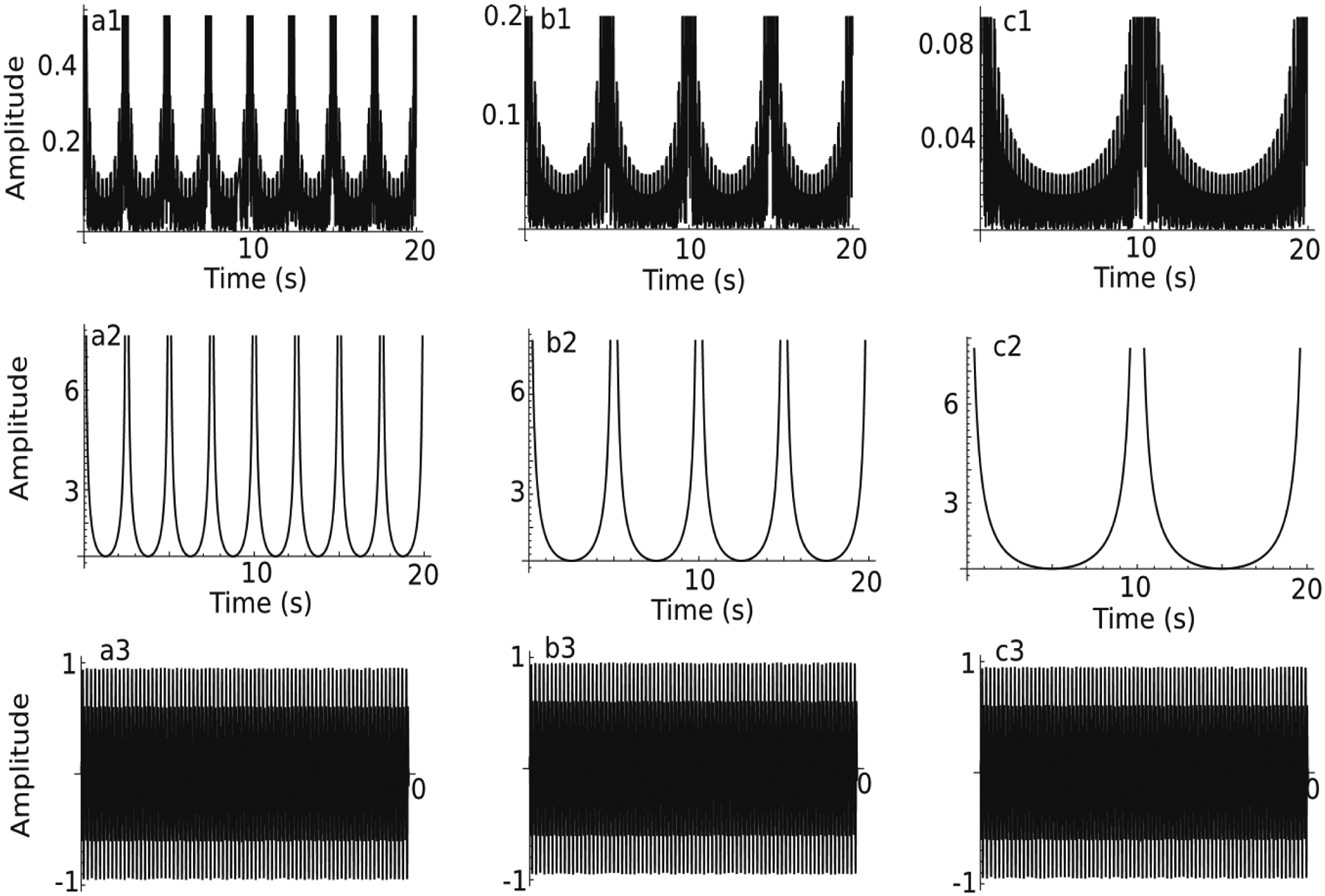
The elements of the theoretical output function of the noise-free SBF-sin (sine-wave) model. Theoretical output function of a noise-free SBF-sin model (equation(2)) for a criterion time T_c = 10 s using a variable number of FC oscillators: 10 (a1), 20 (b1), and 40 (c1). The denominator of the theoretical output function (a2–b2–c2) represents the envelope of the output function shown in panels a1–c1. The numerator of the theoretical output function (a3–b3–c3) represents the fast oscillating part of the output function shown in panels a1–b1–c1 that fills in the envelopes shown in panels a2–b2–c2.

The location of the large-amplitude beats in the envelope of the output function shown in Fig. 2 (a2–b2–c2) is determined by the condition

$$\text{sin}(b_0(t-T_c)/N_{\text{osc}})=0$$ (3)

which leads to b₀|t – T_c|/N_osc = kπ, where k is an integer number representing the number of envelope’s large-amplitude beats over the interval [0, T_c]. The temporal location t of each envelope’s large-amplitude beats is given by

$$\left|t-T_c\right|=k\frac{N_{\mathit{\text{osc}}}}{f_{\mathit{\text{max}}}-f_{\mathit{\text{min}}}}=k\delta T$$ (4)

where δT is the time between two successive large-amplitude beats of the envelope shown in panels a2–b2–c2 of Fig. 2. One gets only one envelope large-amplitude beat over the interval [0, T_c] if k = 1 in equation (3) with the closest spike to the one at T_c located at t = 0 s. Based on equation (3), the minimum number of oscillators required to uniquely resolve the location of T_c, i.e., to get only one largeamplitude beat of the output function over the interval [0, T_c], is

$$N_{\text{osc}}=T_{\text{c}}(f_{\text{max}}-f_{\text{min}})$$ (5)

For the example shown in Fig. 2, with T_c = 10 s and f_max − f_min = 4 Hz, we need at least 40 sine oscillators to resolve such a value of T_c uniquely. For N_osc = 10, the distance between any two peaks of the output function’s envelope is δT = N_osc/(f_max − f_min) = 2.5 s (see Fig. 2a2). For N_osc = 20 (see Fig. 2b2), the distance between any two peaks in the envelope of the output function is δT = N_osc/(f_max − f_min) = 5 s.

The width, σ_out, of the output function is determined from the condition that the output function amplitude at t = T_c + out/2, i.e., out(t = T_c + σ_out/2), is half of its maximum possible amplitude, i.e., ½out(t = T_c).

We also notice that the shape of the theoretical output function (see Fig. 2 panels a1–c1) has a nonzero minimum that is midway between two successive high-amplitude beats. In all our simulations, the maximum amplitude of the theoretical output function (equation (2)) was normalized to the unit. As a result, the normalized minimum amplitude of the theoretical output function was estimated numerically using beta spline envelopes such as those shown in Fig. 3 with long dashed lines. The minimum background activity reflected in the theoretical output function shown in Fig. 2 decreases by increasing the number of FC oscillators. We called the ratio between the normalized maximum amplitude and the minimum amplitude of the output function (see Fig. 3) the SNR.

Figure 3.

The signal-to-noise ratio of a noise-free SBF-sin (sine-wave) model. The theoretical output function (equation (2)), marked with the thin continuous line, was beta spline interpolated (see the thick dashed line) to get the maximum and minimum amplitude of the output signal. The minimum of the envelope decreases, leading to an increase in the SNR, as the number of neural oscillators increases from 20 (a) to the minimum required 40 (b) for a T_c = 10 s (see equation (5)). For more than the minimum number of required oscillators, e.g., 60 oscillators in panel (c), the minimum amplitude of the envelope was measured by averaging over a 3σ interval starting from t = 0 s. As seen in panel (d), the SNR linearly increases with the number of oscillators until the minimum number is reached, and then the SNR saturates. The SNR behavior is consistent over a wide range of criteria from 10 s to 100 s.

To estimate the SNR, we determined the half-width at half-height (HWHH) of the beta spline interpolation of the theoretical output function (see the long dashed lines in Fig. 3), which is related to the standard deviation σ = HWHH/(2√(2 log 2). In the absence of noise, the width of the envelope of the SBF-sin model is constant regardless of the criterion time (see Fig. 3), i.e., it violated scalar property (Oprisan & Buhusi, 2014).

The standard deviation σ was used for computing the background noise amplitude. We could use the envelope’s minimum amplitude as the background activity (noise) value. However, that is the best-case scenario and underestimates the noise level. A more realistic noise estimation is the average around the envelope’s minimum. We used a 3σ interval around the envelope’s minimum to estimate the noise level (see the two vertical arrows marking the gray rectangle of width 3σ in Fig. 3). In the following, we must emphasize that the background activity of the behavioral output curves shown in Fig. 3 will be used to determine the SNR by comparing it against the maximum amplitude of the behavioral output curve. Once the number of PFC oscillators is larger than the minimum necessary to resolve the peak of the theoretical output function (see equation (2)), we measured the SNR 3σ from t = 0 s (see Fig. 3c). As a general trend, the SNR increases linearly with the number of FC oscillators (see Fig. 3d). However, once we reach the minimum number of neural oscillators necessary to resolve the peak of the theoretical output function given by equation (2), any further increase in the number of oscillators has only a subtle effect on SNR, as seen in Fig. 3d.

3.2. Numerical Estimation of the Minimum Number of Oscillators Required for the Timing Task in the Noise-Free SBF-ML Model

The SBF-sin model is helpful because it can lead to general analytic solutions and provide insight into the possible behavior of more complex and biologically realistic implementations of the SBF model (Oprisan & Buhusi, 2014). One such implementation uses Morris and Lecar (1981) spiking neurons instead of sine waved to model neural activity (Oprisan & Buhusi, 2013). As expected, in the SBF-ML model, the noise level decreases with the neural oscillators’ number (see Fig. 4a). The normalized activation function (determined by the FC to BG weights) shows a more substantial peak at the expected criterion time T_c = 20 s with the increasing number of neural oscillators and a simultaneous reduction in background noise level. As with any noise-free SBF model, the standard deviation σ of the smooth envelope of the output function is constant regardless of the criterion time (see Fig. 4b), which violates the scale invariance property of interval timing. We used a smooth Gauss envelope for the numerically generated output function (thick lines in Fig. 4b) to determine the location of the peak response and its standard deviation σ. The average noise level was measured at 3σ from the Gaussian peak (criterion time). The width of the interval over which we computed the average noise level was 2σ, instead of 3σ used in the SBF-sin theoretical prediction. We only used 2σ for the SBF-ML model because the standard deviation of the output function was substantial, and a 3σ interval could not be accommodated numerically for all criteria. We used a 3σ distance from the Gaussian peak to ensure that the average is representative of the background noise (see Fig. 4b).

Figure 4.

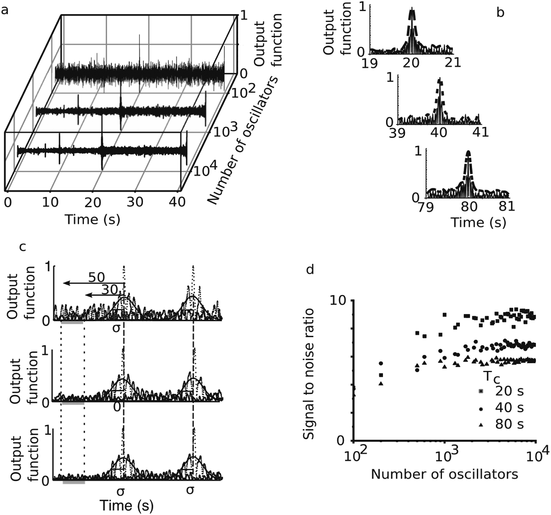
The signal-to-noise ratio of a noise-free SBF-ML (Morris–Lecar) model. The output function of the SBF-ML model shows a more substantial peak at the criterion time T_c = 20 s as we increase the number of neural oscillators (a). For the same criterion time, the background noise amplitude decreases by increasing the number of neural oscillators (a). The output functions of the SBF-ML model (thin continuous lines) were fitted with a smooth beta spline curve (thick long dashed line for T_c = 20 s, thick dotted line for Tc = 40 s, and thick dashed-dotted line for Tc = 80 s) that allowed us to estimate the background noise level (b). To determine the location of the peak of the output function and the standard deviation σ, we used a Gaussian curve (see continuous line) to fit the output of the SBF-ML model (see dotted lines) (c). The noise level was measured by averaging the output function starting 3σ from the criterion time (b). The SNR increases with the number of neural oscillators and eventually saturates (d). For a fixed number of neural oscillators, as the criterion time increases from T_c = 20 s (solid red rectangles) to T_c = 40 s (solid green circles) to T_c = 80 s (solid blue triangles), the SNR decreases.

Similar to the SBF-sin model prediction, we notice that in the SBF-ML model, a more significant number of neural oscillators leads initially to an increase in the SNR followed by its saturation (see Fig. 4c). One notable difference is that the saturation starts at a considerably larger number of neural oscillators, i.e., the SBF-ML model needs a significantly larger number of neural oscillators than the SBF-sin model to resolve the peak of the output function and produce precise timing. ML model neurons have relatively sharp spikes of t_s = 1–3 ms duration, and they are silent for the rest of the firing period. Since the SBF model relies on the set of states of neural oscillators to resolve the output function’s peak, a sine wave offers many discrete values that could encode the state of the FC. For example, an f = 8 Hz sine wave oscillator could be covered by n = 1/(f t_s) = 125 ML neurons, each firing with a spike duration t_s = 1 ms.

This is because an ML model neuron with the same period and a t_s = 1 ms spike duration can only encode one value since the neuron is at rest for the rest of the time. In other words, we need 125 ML neurons to cover the same range of discrete values encoded by a sine wave. We also notice from Fig. 4d that the SNR decreases as the criterion time T_c increases for a fixed number of neural oscillators. The reason is that the quantization (discretization or sampling) error of every cosine wave of the time base with a given number of ML spikes of t_s = 1 ms duration increases with the to-be-timed duration. For example, at the minimum, we could sample any cosine wave only twice during one period and uniquely reconstruct it. However, the quantization error is extremely large as we can only probe two values (out of the infinite number possible in the range (−1, +1). Since the sampled values of the cosine wave serve as the weights for computing the output of the timing model, such a sparse sampling leads to significant errors in representing the state of the FC. Even a very large sampling rate, i.e., many ML neural oscillators, could be insufficient as we increase the criterion time. Such quantization (or sampling) error leads to a more significant error in estimating the state of the FC and a lower SNR, as seen in Fig. 4d.

4. Conclusion

The resource allocation in the interval timing neural network was addressed by determining the minimum number of neural oscillators required to produce precise timing. To find the lower bounds, we used a noise-free SBF model to avoid the complications due to the influence of noise. Based on the SBF-sin model, we found that the required number of oscillators is the product of the criterion time T_c and the frequency range uniformly covered by FC oscillators. As we increase the number of oscillators past the minimum required, the SNR flattens out. As a result, there is no benefit in timing precision by allocating more than the minimum resources needed for the timing task (see Fig. 3d). Based on the numerical simulations of the SBF-ML model, we know that a similar pattern emerges (see Fig. 4d), with the notable difference that the minimum number of required oscillators is one to two orders of magnitude larger than for the same criterion time in the SBF-sin model. A possible explanation is the very different behavior of the action potential in the SBF-sin model compared to SBF-ML. In the SBF-sin model, the membrane potential uniformly samples all amplitudes during a period, whereas an ML model neuron is only active briefly for 1–3 ms and then is silent. An ML action potential, especially for Type I oscillators used here (Ermentrout, 1986; Rinzel and Ermentrout, 1998), looks like a very sharp spike, which could be assimilated to a delta function for long firing periods. As a result, a sine wave sampled every 1–3 ms over its period will require a considerable number of sampling points, which translates into a large number of ML neural oscillators needed for covering the same discrete values of the membrane potential as a sine wave. In a noise-free environment with sine-wave neural oscillators, we found that the model can perform accurate timing with at least N_osc = T_c(f_max − f_min) to encode a duration T_c. However, if spiking neurons are used, like in our SBF-ML model, the numbers above increase by orders of magnitude. This is because every sine wave of frequency f must be sampled with short spikes (action potentials) of duration t_s, which lead to a factor of n = 1/(f t_s). To conclude, the minimum number of spiking ML neural oscillators required is

$$N_{\text{osc}}=T_{\text{c}}\left(f_{\text{max}}-f_{\text{min}}\right)n=T_{\text{c}}\left(f_{\text{max}}-f_{\text{min}}\right)/\left(f_{\text{max}}-t_{\text{s}}\right)=T_{\text{c}}/t_{\text{s}}\left(1-f_{\text{min}}/f_{\text{max}}\right)$$ (6)

For example, a criterion time T_c = 10 s for an SBF-ML implementation with spiking neurons having a spike width of t_s = 1 ms and fitting in the alpha band (f_min = 8 Hz, f_max = 13 Hz) needs at least 3800 neurons. This number increases linearly with the criterion time. However, this is the minimum number of neuronal oscillators required for a noise-free SBF-ML model to maintain an acceptable SNR of the output. It is expected that adding noise increases the number of neural oscillators dedicated to the timing task. Since there are so few neurons (a couple of hundreds to thousands) out of billions of neurons in the prefrontal cortex, which can produce accurate timing, the findings seem consistent with the sparse coding.

We also notice when comparing the SNR for the SBF-sin model (Fig. 3d) against the SBF-ML model (Fig. 4d) that the absolute value of the SNR is significantly smaller in the SBF-ML model. In the SBF-ML model (Fig. 4d), the SNR does not exceed 10 units, which corresponds to 20 log₁₀ SNR = 20 dB. At the same time, from Fig. 3d, we notice that the SNR for the SBF-sin model exceeds 100 units, i.e., more than 40 dB. The SNR for most electrophysiological recordings is right at the edge of 20 dB (Suarez-Perez et al., 2018; Venkatachalam et al., 2011). Behavioral experiments on goldfish (Fay, 2011) showed a similar 20 dB upper bound for SNR. Therefore, the SBF-ML model implemented with realistic biophysical model neurons is within the limits of the SNR reported for biological experiments. We know from the previous implementation that noise is critical for producing the scalar timing in the SBF model (Oprisan & Buhusi, 2013, 2018). Adding noise to the SBF model can only decrease the SNR. Future work will focus on recalculating the lower bounds on the number of neurons required for timing tasks in the presence of noise.

References

- Adler A, Finkes I, Katabi S, Prut Y & Bergman H (2013). Encoding by synchronization in the primate striatum. J. Neurosci, 33, 4854–4866. doi: 10.1523/JNEUROSCI.4791-12.2013. [DOI] [PMC free article] [PubMed] [Google Scholar]
- Anliker J (1963). Variations in alpha voltage of the electroencephalogram and time perception. Science, 140, 1307–1309. doi: 10.1126/science.140.3573.1307. [DOI] [PubMed] [Google Scholar]
- Aschoff J (1989). Temporal orientation: circadian clocks in animals and humans. Anim. Behav, 37, 881–896. doi: 10.1016/0003-3472(89)90132-2. [DOI] [Google Scholar]
- Beiser DG, & Houk JC (1998). Model of cortical-basal ganglionic processing: encoding the serial order of sensory events. Clin. Neurophysiol, 79, 3168–3188. doi: 10.1152/jn.1998.79.6.3168. [DOI] [PubMed] [Google Scholar]
- Boisvert MJ and Sherry DF (2006). Interval timing by an invertebrate, the bumblebee Bombus impatiens. Curr. Biol, 16, 1636–1640. doi: 10.1016/j.cub.2006.06.064. [DOI] [PubMed] [Google Scholar]
- Buhusi CV, Aziz D, Winslow D, Carter RE, Swearingen JE, & Buhusi MC (2009). Interval timing accuracy and scalar timing in C57BL/6 mice. Behav. Neurosci, 123, 1102–1113. doi: 10.1037/a0017106. [DOI] [PMC free article] [PubMed] [Google Scholar]
- Buhusi CV and Meck WH (2002). Differential effects of methamphetamine and haloperidol on the control of an internal clock. Behav. Neurosci, 116, 291–297. doi: 10.1037/0735-7044.116.2.291. [DOI] [PubMed] [Google Scholar]
- Buhusi CV and Meck WH (2005). What makes us tick? Functional and neural mechanisms of interval timing. Nat. Rev. Neurosci, 6, 755–765. doi: 10.1038/nrn1764. [DOI] [PubMed] [Google Scholar]
- Buhusi CV and Meck WH (2010). Timing behavior. In Stolerman IP (Ed.), Encyclopedia of Psychopharmacology, Vol. 2 (pp. 1319–1323). Berlin, Germany: Springer-Verlag. doi: 10.1007/978-3-540-68706-1_275. [DOI] [Google Scholar]
- Canal CE, Stutz SJ, & Gold PE (2005). Glucose injections into the dorsal hippocampus or dorsolateral striatum of rats prior to T-maze training: Modulation of learning rates and strategy selection. Learn. Mem, 12, 367–374. doi: 10.1101/lm.88205. [DOI] [PMC free article] [PubMed] [Google Scholar]
- Catania AC (1970). Reinforcement schedules and psychophysical judgment: A study of some temporal properties of behavior. In Schoenfeld WN (Ed.), The Theory of Reinforcement Schedules (pp. 1–42). New York, NY, USA: Appleton-Century-Crofts. [Google Scholar]
- Cheng K and Westwood R (1993). Analysis of single trials in pigeons’ timing performance. J. Exp. Psychol. Anim. Behav. Process, 19, 56–67. doi: 10.1037/0097-7403.19.1.56. [DOI] [Google Scholar]
- Chiodo LA and Berger TW (1986). Interactions between dopamine and amino acid-induced excitation and inhibition in the striatum. Brain Res, 375, 198–203. doi: 10.1016/0006-8993(86)90976-5. [DOI] [PubMed] [Google Scholar]
- Church RM and Broadbent HA (1990). Alternative representations of time, number, and rate. Cognition, 37, 55–81. doi: 10.1016/0010-0277(90)90018-F. [DOI] [PubMed] [Google Scholar]
- Church RM and Broadbent HA (1991). A connectionist model of timing. In Commons ML, Grossberg S, & Staddon JER (Eds), Neural Network Models of Conditioning and Action (pp. 225–240). Hillsdale, NJ, USA: Lawrence Erlbaum Associates. [Google Scholar]
- Church RM, Meck WH, & Gibbon J (1994). Application of scalar timing theory to individual trials. J. Exp. Psychol. Anim. Behav. Process, 20, 135–155. doi: 10.1037//0097-7403.20.2.135. [DOI] [PubMed] [Google Scholar]
- Church RM, Lacourse DM, & Crystal JD (1998). Temporal search as a function of the variability of interfood intervals. J. Exp. Psychol. Anim. Behav. Process, 24, 291–315. doi: 10.1037/0097-7403.24.3.291. [DOI] [PubMed] [Google Scholar]
- Clarke SP and Ivry RB (1997). The effects of various motor system lesions on time perception in the rat. In Soc. Neurosci. Abstr (Vol. 23, p. 778). [Google Scholar]
- Crystal JD (1999). Systematic nonlinearities in the perception of temporal intervals. J. Exp. Psychol. Anim. Behav. Process, 25, 3–17. doi: 10.1037/0097-7403.25.1.3. [DOI] [PubMed] [Google Scholar]
- Crystal JD, Church RM, & Broadbent HA (1997). Systematic nonlinearities in the memory representation of time. J. Exp. Psychol. Anim. Behav. Process, 23, 267–282. doi: 10.1037/0097-7403.23.3.267. [DOI] [PubMed] [Google Scholar]
- Dallal NL and Meck WH (1993). Depletion of dopamine in the caudate nucleus but not destruction of vestibular inputs impairs short-interval timing in rats. In Soc. Neurosci. Abstr (Vol. 19, p. 1583). [Google Scholar]
- Dews PB (1962). The effect of multiple SΔ periods on responding on a fixed-interval schedule. J. Exp. Anal. Behav, 5, 369–374. doi: 10.1901/jeab.1962.5-369. [DOI] [PMC free article] [PubMed] [Google Scholar]
- Doig NM, Moss J, & Bolam JP (2010). Cortical and thalamic innervation of direct and indirect pathway medium-sized spiny neurons in mouse striatum. J. Neurosci, 30, 14610–14618. doi: 10.1523/JNEUROSCI.1623-10.2010. [DOI] [PMC free article] [PubMed] [Google Scholar]
- Drew MR, Fairhurst S, Malapani C, Horvitz JC, & Balsam PD (2003). Effects of dopamine antagonists on the timing of two intervals. Int. J. Psychophysiol, 75, 9–15. doi: 10.1016/S0091-3057(03)00036-4. [DOI] [PubMed] [Google Scholar]
- Ermentrout GB (1986). Losing amplitude and saving phase. In Othmer HG (Ed.), Nonlinear Oscillations in Biology and Chemistry. Lecture Notes in Biomathematics, vol. 66 (pp. 98–114). Berlin, Germany: Springer. doi: 10.1007/978-3-642-93318-9_6. [DOI] [Google Scholar]
- Fay RR (2011). Signal-to-noise ratio for source determination and for a comodulated masker in goldfish, Carassius auratus. J. Acoust. Soc. Am, 129, 3367–3372. doi: 10.1121/1.3562179. [DOI] [PMC free article] [PubMed] [Google Scholar]
- Gibbon J (1977). Scalar expectancy theory and Weber’s law in animal timing. Psychol. Rev, 84, 279–325. 10.1037/0033-295X.84.3.279. [DOI] [Google Scholar]
- Gibbon J and Allan L (1984). Time perception – introduction. Ann. N. Y. Acad. Sci, 423, 1. doi: 10.1111/j.1749-6632.1984.tb23412.x.6588776 [DOI] [Google Scholar]
- Gibbon J and Church RM (1984). Sources of variance in an information processing theory of timing. In Roitblat HL, Beaver TG, & Terrace HS (Eds), Animal Cognition (pp. 465–488). Hillsdale, NJ, USA: Lawrence Erlbaum Associates. [Google Scholar]
- Gibbon J, Church RM, & Meck WH (1984). Scalar timing in memory. Ann. N. Y. Acad. Sci, 423, 52–77. doi: 10.1111/j.1749-6632.1984.tb23417.x. [DOI] [PubMed] [Google Scholar]
- Groves PM, Garcia-Munoz M, Linder JC, Manley MS, Martone ME, & Young SJ (1995). Elements of the intrinsic organization and information processing in the neostriatum. In Houk JC, Davis JL, & Beiser DG (Eds), Models of Information Processing in the Basal Ganglia (pp. 51–96). Cambridge, MA, USA: MIT Press. [Google Scholar]
- Guckenheimer J, & Holmes P (1983). Nonlinear Oscillations, Dynamical systems and Bifurcations of Vector Fields. New York, NY, USA: Springer-Verlag. [Google Scholar]
- Harrington DL, & Haaland KY (1991). Sequencing in Parkinson’s disease. Abnormalities in programming and controlling movement. Brain Res, 114, 99–115. doi: 10.1093/oxfordjournals.brain.a101870. [DOI] [PubMed] [Google Scholar]
- Houk JC (1995). Information processing in modular circuits linking basal ganglia and cerebral cortex. In Houk JC, Davis JL, & Beiser DG (Eds), Models of Information Processing in the Basal Ganglia (pp. 3–10). Cambridge, MA, USA: MIT Press. [Google Scholar]
- Houk JC, Adams JL, & Barto AG (1995a). A model of how the basal ganglia generate and use neural signals that predict reinforcement. In Houk JC, Davis JL, & Beiser DG (Eds), Models of Information Processing in the Basal Ganglia (pp. 249–270). Cambridge, MA, USA: MIT Press. [Google Scholar]
- Houk JC, Davis JL, & Beiser DG (1995b). Models of Information Processing in the Basal Ganglia. Cambridge, MA, USA: MIT Press. [Google Scholar]
- Izhikevich EM (2000). Phase equations for relaxation oscillators. SIAM J.Appl. Math, 60, 1789–1804. doi: 10.1137/S0036139999351001. [DOI] [Google Scholar]
- Kuramoto Y (1984). Chemical Oscillations, Waves, and Turbulence. New York, NY, USA: Springer-Verlag. [Google Scholar]
- Kuznetsov Yu. A. (2004). Elements of Applied Bifurcation Theory, 3rd ed. New York, NY, USA: Springer-Verlag. [Google Scholar]
- Malapani C, Rakitin B, Levy R, Meck WH, Deweer B, Dubois B, & Gibbon J (1998). Coupled temporal memories in Parkinson’s disease: a dopamine-related dysfunction. J. Cogn. Neurosci, 10, 316–331. doi: 10.1162/089892998562762. [DOI] [PubMed] [Google Scholar]
- Malapani C, Deweer B, & Gibbon J (2002). Separating storage from retrieval dysfunction of temporal memory in Parkinson’s disease. J. Cogn. Neurosci, 14, 311–322. doi: 10.1162/089892902317236920. [DOI] [PubMed] [Google Scholar]
- Maricq AV and Church RM (1983). The differential effects of haloperidol and methamphetamine on time estimation in the rat. Psychopharmacology, 79, 10–15. doi: 10.1007/BF00433008. [DOI] [PubMed] [Google Scholar]
- Maricq AV, Roberts S, & Church RM (1981). Methamphetamine and time estimation. J. Exp. Psychol.. Anim. Behav. Process, 7, 18–30. doi: 10.1037/0097-7403.7.1.18. [DOI] [PubMed] [Google Scholar]
- Matell MS, Chelius CM, Meck WH, & Sakata S (2000). Effect of unilateral or bilateral retrograde 6-OHDA lesions of the substantia nigra pars compacta on interval timing. In Soc. Neurosci. Abstr (Vol. 26, p. 1742). [Google Scholar]
- Matell MS, King GR, & Meck WH (2004). Differential modulation of clock speed by the administration of intermittent versus continuous cocaine. Behav. Neurosci, 118, 150–156. doi: 10.1037/0735-7044.118.1.150. [DOI] [PubMed] [Google Scholar]
- Matell MS and Meck WH (1997). A comparison of the tri-peak and peak-interval procedure in rats: equivalency of the clock speed enhancing effect of methamphetamine on interval timing. In Soc. Neurosci. Abstr (Vol. 23, p. 1742). [Google Scholar]
- Matell MS and Meck WH (2000). Neuropsychological mechanisms of interval timing behavior. Bioessays, 22, 94–103. doi: . [DOI] [PubMed] [Google Scholar]
- Matell MS and Meck WH (2004). Cortico-striatal circuits and interval timing: coincidence detection of oscillatory processes. Cogn. Brain Res, 21, 139–170. doi: 10.1016/j.cogbrainres.2004.06.012. [DOI] [PubMed] [Google Scholar]
- Matell MS, Meck WH, & Nicolelis MAL (2003). Interval timing and the encoding of signal duration by ensembles of cortical and striatal neurons. Behav. Neurosci, 117, 760–773. doi: 10.1037/0735-7044.117.4.760. [DOI] [PubMed] [Google Scholar]
- Meck WH (1983). Selective adjustment of the speed of internal clock and memory processes. J. Exp. Psychol. Anim. Behav. Process, 9, 171–201. [PubMed] [Google Scholar]
- Meck WH (1986). Affinity for the dopamine D2 receptor predicts neuroleptic potency in decreasing the speed of an internal clock. Pharmacol. Biochem. Behav, 25, 1185–1189. doi: 10.1016/0091-3057(86)90109-7. [DOI] [PubMed] [Google Scholar]
- Meck WH (1988). Hippocampal function is required for feedback control of an internal clock’s criterion. Behav. Neurosci, 102, 54–60. doi: 10.1037//0735-7044.102.1.54. [DOI] [PubMed] [Google Scholar]
- Meck WH (1996). Neuropharmacology of timing and time perception. Cogn. Brain Res, 3, 227–242. doi: 10.1016/0926-6410(96)00009-2. [DOI] [PubMed] [Google Scholar]
- Meck WH and Church RM (1987a). Nutrients that modify the speed of internal clock and memory storage processes. Behav. Neurosci, 101, 465–475. doi: 10.1037//0735-7044.101.4.465. [DOI] [PubMed] [Google Scholar]
- Meck WH and Church RM (1987b). Cholinergic modulation of the content of temporal memory. Behav. Neurosci, 101:457–464. doi: 10.1037//0735-7044.101.4.457. [DOI] [PubMed] [Google Scholar]
- Meck WH, Church RM, Wenk GL, & Olton DS (1987). Nucleus basalis magnocellularis and medial septal area lesions differentially impair temporal memory. J. Neurosci, 7, 3505–3511. doi: 10.1523/JNEUROSCI.07-11-03505.1987. [DOI] [PMC free article] [PubMed] [Google Scholar]
- Miall C (1989). The storage of time intervals using oscillating neurons. Neural Comput, 1, 359–371. doi: 10.1162/neco.1989.1.3.359. [DOI] [Google Scholar]
- Morris C and Lecar H (1981). Voltage oscillations in the barnacle giant muscle fiber. Biophys. J, 35, 193–213. doi: 10.1016/S0006-3495(81)84782-0. [DOI] [PMC free article] [PubMed] [Google Scholar]
- Neil DB and Herndon JG Jr (1978). Anatomical specificity within rat striatum for the dopaminergic modulation of DRL responding and activity. Brain Res, 153, 529–538. doi: 10.1016/0006-8993(78)90337-2. [DOI] [PubMed] [Google Scholar]
- Olton DS, Wenk GL, Church RM, and Meck WH (1988). Attention and the frontal cortex as examined by simultaneous temporal processing. Neuropsychologia, 26, 307–318. doi: 10.1016/0028-3932(88)90083-8. [DOI] [PubMed] [Google Scholar]
- Oprisan SA and Buhusi CV (2011). Modeling pharmacological clock and memory patterns of interval timing in a striatal beat-frequency model with realistic, noisy neurons. Front. Integr. Neurosci, 5:52. doi: 10.3389/fnint.2011.00052. [DOI] [PMC free article] [PubMed] [Google Scholar]
- Oprisan SA and Buhusi CV (2013). How noise contributes to time-scale invariance of interval timing. Phys. Rev. E, 87, 052717. doi: 10.1103/PhysRevE.87.052717. [DOI] [PMC free article] [PubMed] [Google Scholar]
- Oprisan SA and Buhusi CV (2014). What is all the noise about in interval timing? Philos. Trans. R. Soc. Lond. B Biol. Sci, 369, 20120459. doi: 10.1098/rstb.2012.0459. [DOI] [PMC free article] [PubMed] [Google Scholar]
- Oprisan SA, Aft T, Buhusi M, & Buhusi CV (2018a). Scalar timing in memory: A temporal map in the hippocampus. J. Theor. Biol, 438:133–142. doi: 10.1016/j.jtbi.2017.11.012. [DOI] [PMC free article] [PubMed] [Google Scholar]
- Oprisan SA, Buhusi M, & Buhusi CV (2018b). A population-based model of the temporal memory in the hippocampus. Front. Neurosci, 12, 521. doi: 10.3389/fnins.2018.00521. [DOI] [PMC free article] [PubMed] [Google Scholar]
- Rakitin BC, Gibbon J, Penney TB, Malapani C, Hinton SC and Meck WH (1998). Scalar expectancy theory and peak-interval timing in humans. J. Exp. Psychol.: Anim. Behav. Process, 24, 15–33. doi: 10.1037/0097-7403.24.1.15. [DOI] [PubMed] [Google Scholar]
- Rammsayer TH (1993). On dopaminergic modulation of temporal information processing. Biol. Psychol, 36, 209–222. doi: 10.1016/0301-0511(93)90018-4. [DOI] [PubMed] [Google Scholar]
- Rinzel J and Ermentrout B (1998). Analysis of neural excitability and oscillations. In Koch C and Segev I (Eds), Methods in Neuronal Modeling (pp. 135–169). Cambridge, MA, USA: MIT Press. [Google Scholar]
- Rizzuto DS, Madsen JR, Bromfield EB, Schulze-Bonhage A, Seelig D, Aschenbrenner-Scheibe R, & Kahana MJ (2003). Reset of human neocortical oscillations during a working memory task. Proc. Natl Acad. Sci. U. S. A, 100, 7931–7936. doi: 10.1073/pnas.0732061100. [DOI] [PMC free article] [PubMed] [Google Scholar]
- Roberts S (1981). Isolation of an internal clock. J. Exp. Psychol.: Anim. Behav. Process, 7, 242–268. doi: 10.1037/0097-7403.7.3.242. [DOI] [PubMed] [Google Scholar]
- Schlauch RS, Harvey S, & Lanthier N (1995). Intensity resolution and loudness in broadband noise. J. Acoust. Soc. Am, 98, 1895–1902. doi: 10.1121/1.413375. [DOI] [PubMed] [Google Scholar]
- Schneider BA (1969). A two-state analysis of fixed-interval responding in pigeons. J. Exp. Anal. Behav, 12, 667–687. doi: 10.1901/jeab.1969.12-677. [DOI] [PMC free article] [PubMed] [Google Scholar]
- Staddon JER (1965). Some properties of spaced responding in pigeons. J. Exp. Anal. Behav, 8, 19–27. doi: 10.1901/jeab.1965.8-19. [DOI] [PMC free article] [PubMed] [Google Scholar]
- Suarez-Perez A, Gabriel G, Rebollo B, Illa X, Guimerà-Brunet A, Hernández-Ferrer J, Martínez MT, Villa R, & Sanchez-Vives MV (2018). Quantification of signal-to-noise ratio in cerebral cortex recordings using flexible MEAs with co-localized platinum black, carbon nanotubes, and gold electrodes. Front. Neurosci, 12, 862. doi: 10.3389/fnins.2018.00862. [DOI] [PMC free article] [PubMed] [Google Scholar]
- Talton LE, Higa JJ, & Staddon JER (1999). Interval schedule performance in the goldfish Carassius auratus. Behav. Proc, 45, 193–206. [DOI] [PubMed] [Google Scholar]
- Treisman M (1963). Temporal discrimination and the indifference interval. Implications for a model of the internal clock. Psychol. Monogr, 77, 1–31. doi: 10.1037/h0093864. [DOI] [PubMed] [Google Scholar]
- Umemiya M, & Raymond LA (1997). Dopaminergic modulation of excitatory postsynaptic currents in rat neostriatal neurons. J. Neurophysiol, 78, 1248–1255. doi: 10.1152/jn.1997.78.3.1248. [DOI] [PubMed] [Google Scholar]
- Venkatachalam KL, Herbrandson JE, & Asirvatham SJ (2011). Signals and signal processing for the electrophysiologist. Circ. Arrhythm. Electrophysiol, 4, 965–973. doi: 10.1161/CIRCEP.111.964304. [DOI] [PubMed] [Google Scholar]
- Wearden JH and Doherty MF (1995). Exploring and developing a connectionist model of animal timing: Peak procedure and fixed-interval simulations. J. Exp. Psychol.. Anim. Behav. Process, 21, 99–115. doi: 10.1037/0097-7403.21.2.99. [DOI] [Google Scholar]
- Winfree AT (2001). The Geometry of Biological Time. New York, NY, USA: Springer-Verlag. [Google Scholar]