

Abstract
Mutant dynamics in fragmented populations have been studied extensively in evolutionary biology. Yet, open questions remain, both experimentally and theoretically. Some of the fundamental properties predicted by models still need to be addressed experimentally. We contribute to this by using a combination of experiments and theory to investigate the role of migration in mutant distribution. In the case of neutral mutants, while the mean frequency of mutants is not influenced by migration, the probability distribution is. To address this empirically, we performed in vitro experiments, where mixtures of GFP‐labelled (“mutant”) and non‐labelled (“wid‐type”) murine cells were grown in wells (demes), and migration was mimicked via cell transfer from well to well. In the presence of migration, we observed a change in the skewedness of the distribution of the mutant frequencies in the wells, consistent with previous and our own model predictions. In the presence of de novo mutant production, we used modelling to investigate the level at which disadvantageous mutants are predicted to exist, which has implications for the adaptive potential of the population in case of an environmental change. In panmictic populations, disadvantageous mutants can persist around a steady state, determined by the rate of mutant production and the selective disadvantage (selection‐mutation balance). In a fragmented system that consists of demes connected by migration, a steady‐state persistence of disadvantageous mutants is also observed, which, however, is fundamentally different from the mutation‐selection balance and characterized by higher mutant levels. The increase in mutant frequencies above the selection‐mutation balance can be maintained in small () demes as long as the migration rate is sufficiently small. The migration rate above which the mutants approach the selection‐mutation balance decays exponentially with . The observed increase in the mutant numbers is not explained by the change in the effective population size. Implications for evolutionary processes in diseases are discussed, where the pre‐existence of disadvantageous drug‐resistant mutant cells or pathogens drives the response of the disease to treatments.
Keywords: clonal composition, fragmented populations, mathematical models, migration, mutant dynamics
In large populations, disadvantageous mutants can persist around a steady state, determined by the rate of mutant production and the selective disadvantage (selection‐mutation balance). In a fragmented system that consists of subpopulations connected by migration, a steady‐state persistence of disadvantageous mutants is also observed, which, however, is fundamentally different from the mutation‐selection balance and characterized by higher mutant levels.

1. INTRODUCTION
Understanding the principles of mutant dynamics has been a major focus in evolutionary biology. Generation and spread of mutants is central to adaptation, where beneficial mutants tend to fix while deleterious mutants are gradually removed from the population. These processes depend on the environment and are guided by forces of selection, the rate of mutation, genetic drift and the population structure.
Population structure is an important determinant of the evolutionary trajectories (Levin, 1974; Levin & Powell, 1993). Evolutionary dynamics in fragmented populations are of interest for questions connected to ecology and ecological conservation (Earn et al., 2000; Kalarus & Nowicki, 2015; Lander et al., 2019; Prugh et al., 2008; Rochat et al., 2017; Rubinoff & Powell, 2004; Thomas et al., 2001). Human interference as well as natural factors may fragment habitats and isolate subpopulations of a species from the rest, thus influencing genetic variability and species survival. Population genetics in structured populations has been applied to studies of island biogeography, dynamics of species living in patchy environments, extinction and recolonization, see for example (Hanski, 1998; Wade & McCauley, 1988). Another area where population fragmentation is of great importance is host‐associated microbiomes. Spatial structures are generated by host anatomy and physiology; examples include gastrointestinal crypts (Fung et al., 2019) and skin pores (Conwill et al., 2022). Understanding the microbial evolution in structured populations is critical for modelling community diversity and stability, species coexistence, and predicting the response of microbiomes to treatments. Further applications to biomedical problems are discussed below.
Mathematical models have been an important component of research into mutant dynamics. Different types of evolutionary models have been explored; most relevant for the current paper are the Moran process (Moran, 1958; Moran, 1962) and the Wright‐Fisher model (Wright, 1931) that assume constant population sizes. Various evolutionary measures have been considered, including the average frequency of mutants at a given time or population size, the fixation probability of mutants and the average time to fixation for mutants of varying relative fitness (Loewe & Hill, 2010; Kareiva et al., 1990; Kimura, 1962; López‐Cortegano et al., 2019; Patwa & Wahl, 2008; Whitlock, 2003).
Evolution in fragmented populations is described by models that are sometimes referred to as structured or subdivided population models, as well as patch or deme models (Hanski, 1998; Hanski & Gilpin, 1991; Levin, 1974; Levin & Powell, 1993; Levins, 1969; Moran, 1962). These models describe a group of distinct, spatially separated populations of the same type. Some amount of interaction between the separate groups occurs via migration of individuals from one group to another, and the dynamics within a single group of individuals is generally assumed to be non‐spatial (Hauert & Imhof, 2012; Levins, 1969; Moran, 1962; Wakeley & Takahashi, 2004). Migration of individuals can either occur to the nearest neighbouring regions (spatially restricted), or individuals can migrate to any region in the system. A higher rate of migration decreases population fragmentation because it results in each region's dynamics becoming dependent on a larger portion of the overall population and thus in better mixing of individuals (Hanski & Gilpin, 1991; Moran, 1962; Wakeley & Takahashi, 2004; Wright, 1931). The term “metapopulation models” is often reserved to describing the dynamics with local extinctions and re‐colonization, see for example (Cherry, 2003; Hanski, 1998; Levin, 1974; Levin & Powell, 1993; Slatkin, 1977; Wade & McCauley, 1988).
Mathematical patch models with different assumptions on structure and migration between groups have been studied in the context of evolutionary dynamics. A number of important results about the effect of fragmentation and structure on mutant dynamics have been established. Commonly, it is found that the fixation probability of a mutant is largely independent of migration (depending on the explicit model assumptions) (Maruyama, 1970; Maruyama, 1974; Wakeley & Takahashi, 2004), but that other quantities such as the time to fixation and effective population size can vary based on model structure (Slatkin, 1981; Whitlock, 2003). The distribution of mutant numbers in individual demes has been studied in different contexts, starting with the seminal paper by Wright (Wright, 1931), which gave rise to the shifting balance theory of evolution. Further developments include both discrete (Wright‐Fisher) and overlapping (Moran) models of population dynamics and different assumptions on the migration process, see for example (Hanski & Gilpin, 1991; Hauert & Imhof, 2012; Moran, 1962; Wakeley & Takahashi, 2004). It was found that generally, migration among demes transforms the probability distribution of mutant frequency in a deme from bimodal to unimodal. Another set of results comes from the diffusion approximation that describes selection and drift of mutants in subdivided populations. In Cherry & Wakeley (2003) and Wakeley (2003), a Wright‐Fisher process in a subdivided population with inter‐deme migrations is considered, while in Wakeley & Takahashi (2004), the local dynamics are described by a Moran process. Analytical expressions for the effective population size are derived. It is shown that although the form of the diffusion approximation is equivalent between a structured and panmictic population, fragmentation can significantly increase the effective population size and the variance of allele frequencies.
The interplay between patch dynamics and traits or alleles has also been previously studied in multiple experimental contexts (Chakraborty et al., 2021; Fusco et al., 2016; Kerr et al., 2006; Lavigne et al., 2001). For instance, Kerr et al. (2006) identified path‐dependent migration effects in the eco‐evolutionary dynamics of E. coli‐T4 phage co‐cultures. Excitingly, recent work on range expansions in asexually reproducing microbes has shown that an excess of spontaneous mutations (relative to Luria‐Delbruck expectations) is generated during spatial range expansions by allele surfing (Fusco et al., 2016).
While several aspects of mutant dynamics in fragmented populations have been mathematically elucidated, there still remain open theoretical questions and experimental gaps, some of which we address in this paper. (i) From an experimental point of view, to the best of our knowledge, direct tests of model predictions regarding mutant distributions in fragmented asexual populations in the presence and absence of migration are lacking. Here, we provide an experimental test of fundamental model predictions about mutant distributions for neutral mutants, using a system where GFP‐labelled and unlabelled murine cell lines (“mutant” and “wild‐type”) are co‐cultured in 96‐well plates, and migration is mimicked by swapping cells between demes (wells) with a pipette. This system does not contain de novo mutant production, and the experimental results are interpreted with a corresponding Moran process model, which reproduces previous theoretical insights and is found to be consistent with the data. (ii) The model is then used to extend this analysis assuming de novo mutant production and different mutant fitness. In particular, we study the perceived “selection‐mutation balance” in populations. This refers to the persistence of disadvantageous mutants around a steady state in a population of wild‐types at equilibrium, the level of which can be calculated and is determined by the mutation rate and the degree of the selective disadvantage. We show that for a fragmented habitat, disadvantageous mutants can also persist at a steady‐state level similar to the selection‐mutation balance in a panmictic population, but that there is a fundamentally different scenario in which the expected number of mutants at the steady state can be significantly higher. Our results demonstrate that the previously obtained change in the effective population size of fragmented populations is not enough to explain the change in the level at which the disadvantageous mutants persist. This has implications for understanding the adaptive potential of a population in response to environmental change, with broad applicability ranging from ecological systems to biomedical problems, such as the emergence of drug‐resistant mutants.
2. METHODS
2.1. Experiments with neutral mutants
To address the existing gap in the literature concerning studies of neutral mutant dynamics in fragmented populations in the presence and absence of migration, we performed experiments that represent an in vitro comparison to the mathematical model presented in the following section. To create a system representing neutral migration we mixed GFP labelled mammalian cells with unlabeled cells. This suspension of mammalian cells could be propagated in the wells of a 96 well plate. By systematically transferring small volumes of the cell suspension, we experimentally simulated migration between wells. Cells were continually maintained at confluent cell population densities to mimic the Moran process. The proportion of mutants in the wells both with and without migration of cells between wells was assessed at the end of the experiment. Further details on the in vitro experiments are presented below.
2.1.1. Experimental details
In total, 96 demes (wells) were filled with cells. Cell types were wild type and mutant, which were neutral with respect to one another. To create this model, we transduced murine Ba/F3 cells (DSMZ; ACC‐300) with green fluorescent protein (GFP). GFP+ cells were mixed with wild‐type Ba/F3 cells into populations of approximately 0.1% and 1% GFP+. Ba/F3 populations were maintained in RPMI 1640 Medium (Sigma Aldrich), supplemented with 10% FBS (Fisher), 10 ng/ml IL‐3 (PeproTech), 100 U/ml penicillin and 100 μg/ml streptomycin (Life Technologies). The control condition was no migration and the experimental condition was migration between demes, which was performed by swapping cells between demes using a pipette. Four total experiments were performed, with both conditions starting at approximately initial mutants and also at initial mutants in all demes. Wells in each plate were diluted twice daily with fresh medium on a 16/8 h time interval to maintain competition at high confluence, with one plate from each mixed population subject to migration events at these intervals. All wells were maintained at 200 μl – dilutions with fresh medium were performed to maintain cell confluency at stationary phase and replenish nutrients. This was done to approximate a Moran process and allow for continuous culture, and it was a significant challenge. Throughout the experiment, maximum population densities were adjusted based on viability, to maintain population density and competition. Migration events were performed immediately prior to viability dilutions on one plate of each GFP+ population through the duration of the experiment. Each well in a row was thoroughly homogenized, and 5 μl of each well's 200 μl volume was transferred to the vertically adjacent well. Receiving wells were then homogenized and 5 μl was transferred to the next adjacent well; this process was repeated until all eight rows had received volume from its adjacent upstream row and transferred to its downstream adjacent row.
2.2. Mathematical modelling
To study the role of population fragmentation and migration in evolution, we will consider a population of asexually reproducing (haploid) individuals of two types, which we refer to as “wild types” and “mutants”, see Figure 1. The total population of individuals is split into demes of individuals each, as in for instance (Hauert & Imhof, 2012). We assume a finite island model, where all demes are equidistant. Competition is implemented by assuming that (neutral or deleterious) mutants may have relative fitness (denoted by ) that is not necessarily equal to the fitness of the wild types (assumed to be ). De novo mutations are included through forward mutation (with probability per division of a wild type cell) and back‐mutation (with probability per division of a mutant cell, further details included in Section 2.2.1). Migration is modelled in the following way. A single migration event is attempted with probability and performed by randomly selecting two demes, then randomly selecting individuals from each and swapping them with each other; migration updates are completed each time.
FIGURE 1.

A schematic illustrating the mathematical model. (a) General model structure: Each rectangle represents a deme, and green (red) circles represent wild‐type (mutant) individuals. Two‐sided arrows represent random swap‐migration events within randomly chosen pairs of demes. (b) Details of a swap migration event: groups of cells are randomly selected within two demes, and exchanged. As a result of this particular event, the number of mutants in the top deme decreased, and the number of mutants in the bottom deme increased by 2.
The dynamics are set up in the following way: First, a migration update is performed, where individuals have a chance to swap demes. This is followed by a birth‐death update in all demes. Further details on birth‐death updates are given in Section 2.2.1, and on migration in Section 2.2.2; Table 1 lists all the model parameters. We run simulations until long‐term dynamics have been established and (quasi)‐stationary states (mutant extinction/fixation or a stable average number of mutants within individual demes and the overall system) have been reached.
TABLE 1.
Description of model parameters
| Notation | Description | |
|---|---|---|
|
|
Number of demes | |
|
|
Constant number of individuals in each deme | |
|
|
Constant total number of individuals in overall population | |
|
|
Fitness of the mutant individuals | |
|
|
Rate of forward mutation wild type mutant | |
|
|
Rate of back‐mutation wild type mutant | |
|
|
Migration probability | |
|
|
Number of individuals exchanged during a swapping event | |
|
|
Number of swaps that occur during a migration event | |
|
|
Selection mutation balance in each deme |
2.2.1. The Moran process
Within each deme, we model the stochastic birth‐death dynamics by using the well‐known Moran process (see e.g. Moran, 1958; Moran, 1962). Therefore, the population size of each deme as well as the total population size remains constant. The process of de novo (forward and/or backward) mutation may be included in our framework. De novo mutation occurs during reproduction, so for instance if a wild‐type cell is chosen for reproduction, there is a chance of faithful reproduction and a chance to create a mutant. If a mutant cell divides, it creates a wild‐type offspring with probability (and a mutant offspring with probability ).
In the absence of de novo forward mutation (), the model has only one absorbing state, given by mutant extinction in all demes. Similarly, in the absence of de novo back mutation (), mutant fixation in all demes is the only absorbing state. With the inclusion of both forward and back mutation, there are no absorbing states (Moran, 1958). In the absence of migration, the stationary probability distribution in an individual deme can be calculated. For example, in the regime where mutant fixation happens on a much faster time‐scale than mutant production, a simple expression for the stationary probability can be derived. Denoting by the probability to have mutants in the deme, we have
| (1) |
with the probability of the other states being of the order of the mutation rate, which is described in further detail in Section 2.2.3. This is similar to previous approximations of the stationary distribution for the Moran process with de novo mutation and selection and under various conditions, see for instance (Ewens, 2007; Fudenberg et al., 2006; Karlin & McGregor, 1962; Moran, 1962; Wakeley & Takahashi, 2004). Another useful quantity is the selection‐mutation balance, which is given (for an individual deme, in the limit of small mutation rates) by
| (2) |
this quantity represents the number of (negatively selected, ) mutants, in the Moran process with de novo mutations, which corresponds to an equal probability to increase and decrease this number in a single birth‐death update. This quantity is also identical to the classical expression of the expected number of deleterious mutations at mutation‐selection balance. Section 2.2.3 (see also (Ewens, 2007; Fudenberg et al., 2006; Moran, 1962)) provides details of the calculations for expressions (1) and (2), as well as higher order approximations.
The process of Moran birth‐death updates within an individual deme is set up as follows: Suppose the number of mutants is given by (and thus the number of wild type individuals is given by ). For each time step, a cell is chosen randomly to die and a cell is chosen based on fitness to reproduce. 1 Therefore, the chance that a mutant is chosen to reproduce is , and the chance that a wild type is chosen to reproduce is . This is a Markov process, where the states of the model (the number of mutants in the deme) are integers . This model has a tridiagonal transition matrix. Let us define
| (3) |
to be the probabilities to increase and decrease the number of mutants starting from mutants, in one step. Then we have
Let us denote the probability to have mutants at time in a deme as , with , . The row vector contains this information for each discrete time‐step, . The initial condition is
In the absence of migration, we have (in matrix form)
If both populations reproduce faithfully (), we have two absorbing states, (mutant extinction) and (mutant fixation) (Moran, 1962). Let denote the probability for mutants to reach fixation given that we start with mutants. We have
2.2.2. Modelling migration
We assume a migration update is attempted at each step with some migration probability . We assume that at each migration update, individuals are randomly picked from one deme and replaced with individuals randomly selected from the second deme. In some simulations, to increase the intensity of migration, we repeated this procedure times for each migration update. We assume that the probability of migration applies to all swap events jointly, and thus that swap events occur with probability , and no swap events occur with probability . and are non‐negative integers that we set before performing a simulation.
To incorporate migration, let us assume that a migration update precedes a Moran update. Then we can write
| (4) |
where denotes the transition matrix associated with migrations. In order to formulate this transition matrix, we will need the Hypergeometric distribution, which describes the probability of picking mutants in draws without replacement, if the total number of mutants is out of individuals:
The probability to change the number of mutants from to in a population characterized by vector is given by
Here, we assume that the population containing mutants loses mutants to another deme and gains mutants from the other deme; we sum over all possible values of , and note that
which gives us the expression for . The probability to lose individuals is . The probability to gain individuals is calculated as follows: the donor deme is assumed to contain mutants (probability ), because all individuals are assumed to obey the same laws and the number of mutants in the deme at time are drawn from the same probability distribution, . The probability to gain mutants from a deme containing mutants is , and to get the total probability of gaining individuals, we sum over all .
Finally, the transition matrix for the migration step is given by
where is the Kronecker delta.
The steady state, , satisfies the following equation:
| (5) |
where
2.2.3. The stationary probability distribution and the selection‐mutation balance in the absence of migration
In the presence of de novo forward and back mutations, let us determine the stationary probability distribution for the number of mutants. Let us suppose the stationary probability distribution is given by with
| (6) |
The components satisfy the following equation
| (7) |
where and the transition probabilities are given by Equation 3. Let us suppose that the mutation rates are small compared with and the inverse of the deme size , and denote
. Solving Equation 7 in the zeroth order (i.e. under the assumption of no de novo mutations, setting ), we obtain for , with probabilities and undefined. To find the approximate solution under the assumption of small mutation rates, we go to the first order in . Let us set
Taking into account only the terms of order in Equation 7, we obtain a degenerate system of equations for unknowns . The additional condition in given by Equation 6 and in the lowest order in reduces to . The solution is similar to what is found by (Ewens, 2007; Fudenberg et al., 2006) in similar models, and is given by
| (8) |
| (9) |
In particular, in the absence of de novo back mutations, the system converges to the state (mutant fixation), and in the absence of de novo forward mutations, we have (mutant extinction). If we include higher order terms, then the stationary distribution for the intermediate states is given by
| (10) |
Approximation (8)–(9) can also be obtained from the following simple consideration. Let us assume that the system spends most of the time in “pure” states (i.e. in state or in state ), which is the consequence of the time‐scale separation: the waiting time to obtain a de novo mutation must be much longer than the typical time of mutant fixation. Then we can establish the balance of the following two processes: (1) If the system is in state (denote this probability by ), then the transition to state happens at rate , which is the product of the mutant production rate, , and the probability of a single mutant fixation given by with . (2) On the other hand, the probability of finding the system in state is , and the rate at which the system leaves and gets fixed at is given by multiplying the rate of wild type production () by the probability of a wild‐type fixation (), where we replace with , which is the relative fitness of the wild type compared to that of mutants. We obtain the equation
whose solution is given by Equation 8.
To calculate the selection‐mutation balance, we solve the equation for and obtain Equation 2, where we used the largest contribution in (this is also the exact solution for the selection‐mutation balance in the case of only forward mutation). We also note that back mutation does not effect the selection‐mutation balance as long as . The exact solution for the selection‐mutation balance is given by
| (11) |
In the case that the two types are neutral with respect to each other (), we again solve the equation for and as in (Moran, 1962) obtain
| (12) |
3. RESULTS
3.1. Population fragmentation changes mutant distribution for neutral mutants
To motivate this study, we performed some simple experiments that examined the role of fragmentation and migration in neutral mutant dynamics. Ninety‐six wells were filled with cells such that each well contained 1% of (neutral) mutants. The process of cell migration was implemented by swapping a small percentage of cells between demes by using a pipette (which is described in more detail in Section 2.1 and in Appendix S2 Section 1). The number of mutants in the wells was assessed at the end of the experiment and compared with the control condition with no migration. The resulting experimentally obtained distribution of the mutant numbers is shown in Figure 2 and Figure S1, where we plot the percent mutant contents in the ninety‐six demes in the form of histograms. Figure 2 shows experimental results for the 1% mutants initial condition and Figure S1 shows experimental results for both the 0.1% and 1% mutants initial conditions.
FIGURE 2.

Effect of migration on neutral mutant distribution, experimental results. The blue bars represent the control condition without migration between the wells, the yellow bars represent the experimental condition with migration, and the grey colour denotes the overlap. The initial condition was mutants in each well. The average percent of mutants in each well without migration is 1.03%, and with migration is 1.13% (not significantly different using the T test, p > 0.1). The Kolmogorov–Smirnov test between the two distributions gives a p‐value of about , which suggests that the distributions are significantly different. The skewness without migration is 0.89, and with migration, it is much smaller at 0.07. Full experimental results are shown in Figure S1.
We observed that while the mean number of mutants in the absence and in the presence of migration was the same, the distribution was significantly different; in particular, the distribution without migration had a much larger skewness, while in the presence of migration, it was more symmetric (Figure 2). Specifically, the average percent of mutants without migration is , and with migration is , which is not significantly different using the T test (p > 0.1). However, the Kolmogorov–Smirnov test between the two distributions gives a p‐value of about , which suggests that the distributions are significantly different. The skewness for the experiment without migration is 0.89, and with migration it is much smaller at 0.07.
To explain these observations and extend the results to other conditions, we began by analysing the dynamics of neutral mutants ().
3.1.1. Unimodal versus bimodal mutant distribution in the absence of de novo mutations
To reproduce the experimental set‐up, we assumed that there is no de novo mutation, and started with some small initial number of mutants in each deme (). In order to analyse the effect of migration/population fragmentation, we ran simulations with and without migration of cells between the distinct demes, a description of the mathematical model can be found in Section 2.
As in the experimental results, in both the model simulations and analysis, we found that the mean percent of neutral mutants is independent of migration, and is equal to the initial ratio of mutants in the system. This is because the transition probabilities are symmetric, see Equation 3 and Section 2 in the Appendix S2 for details. Furthermore, as the wild type and mutant are neutral, the probability for the mutant to fix within the system (assuming a non‐zero migration rate) is equal to the initial frequency of mutants in the system (although the time to such fixation depends on migration (Slatkin, 1981; Whitlock, 2003)). This is because in the context of a symmetric random walk, the fixation (i.e. absorption at the upper boundary) probability is proportional to the initial condition, see Appendix S2 Section 2 and (Maruyama, 1970; Moran, 1958; Moran, 1962).
On the other hand, the distribution of the frequency of mutants in the system and the dynamics within individual demes are significantly influenced by the presence of migration (Figure 3). Starting from a delta‐like distribution (as initially all demes contain mutants), the distributions get wider with time and eventually reach a quasi‐stationary distribution. In the absence of migration (Figure 3a), the dynamics of each deme are independent from one another. Since the probability of fixation is simply the initial fraction of mutants (), there is a large chance (given by ) of mutant extinction in each deme. Therefore, the probability distribution of the number of mutants in each deme becomes flatter and develops a skew to the right, as most demes will trend towards mutant extinction, while a few will trend towards mutant fixation (i.e. a bimodal distribution, with modes at mutant extinction () and fixation ()). Eventually, as time , all demes will be fixed at either mutant extinction or fixation. In the presence of migration (panel (b)), the dynamics of each deme are no longer independent from one another. As was similarly found in (Hanski & Gilpin, 1991; Hauert & Imhof, 2012; Moran, 1962; Wakeley & Takahashi, 2004; Wright, 1931), migration makes all the demes look more similar to each other, resulting in a one‐humped (unimodal) distribution. These results match well with in vitro experimental simulations of the computational model, which are shown in Figure 2 (see also Appendix S2 Section 1). Note that while the figure shows a long‐term state, this is not an equilibrium, and the only outcomes as time is mutant fixation or mutant extinction in the whole system (individual demes, if ) because there is no de novo mutation (Hauert & Imhof, 2012; Moran, 1962).
FIGURE 3.

Stochastic simulations (histograms) and iterations of Equation 4 (blue lines). Panel (a) represents the absence () and panel (b) represents the presence () of migration. The probability distributions are presented at several moments of time ( in each plot corresponds to the number of discrete Moran steps). The rest of the parameters are and .
In addition to the extremes of no migration or a large amount of migration (where the system is well‐mixed), we also investigate other regimes where there is some intermediate level of migration of individuals between the demes in the system. Figure S4 shows the timeevolution of the mutant probability distributions obtained by iterating Equation 4 (see panels (a–c) for three different values of ), and then by plotting the resulting quasi‐stationary probability distributions (panel (d)). Here we see that the effect of the Moran process is to “make” the probability distribution bimodal, and the effect of migration is to “make” it unimodal. The result is a trade‐off of the two tendencies, and depending on the amount of migration, the distribution shape changes accordingly.
3.1.2. Quasi‐stationary distributions become stationary in the presence of de novo mutation
Next, we expand the theory beyond the experimental conditions of Figure 2 to include the effect of de novo mutations. Since mutants are now generated stochastically, we alter the initial conditions to start with the wild type fixed in all demes (). In the case of only forward mutation, the mutant will be created via mutation more often than the wild type. This mutational bias results in the neutral mutant () fixing quickly in the entire population (see Figure S6a,b). On average, the time to fixation decreases with increasing migration, as faster migration results in more frequent introduction of the mutant into all of the demes, see (Hanski, 1998; Slatkin, 1981; Wakeley & Takahashi, 2004; Whitlock, 2003).
In the case of both forward and back de novo mutation, the dynamics are more complex. Figure 4a shows simulations representing demes of 20 individuals each, after iterations with varying rates of migration. The histograms represent the number of neutral mutants per deme. In the absence of migration (left), the number of mutants will drift around, becoming extinct or fixed within a deme. In a highly fragmented population, this will happen more often, and the mutant will be at the extinction/fixation long‐term state most of the time. Increasing migration (and/or decreasing population fragmentation by increasing the size of the demes, not shown) will result in fluctuation around the equilibrium value (Equation 12) in each deme (Figure 4a, right). As in the simulations without de novo mutation, if the rate of forward and back mutation is equal (), then migration does not change the expected mean number of neutral mutants (as the stationary distribution is symmetric around the selection‐mutation balance of 50% mutants, see Figures S5 and S6c,d). If the rate of forward and back mutation is not equal (, then the expected level of mutants is given by (see Equation 12 and Moran, 1962 for details of this calculation).
FIGURE 4.

Histograms for the number of mutants per deme in the absence () and presence () of migration, after Moran iterations. (a) Neutral mutant () with both forward and back mutation (), see Figure S5 for intermediate migration cases; (b) disadvantageous mutant () with forward mutation only (, ), see Figure S12 for intermediate migration cases; (c) disadvantageous mutant (), with forward and backward mutation (), see Figure S13 for intermediate migration cases. The horizontal axis is the number of mutants and the vertical axis is the number of demes at that number of mutants. The vertical lines in the right panels represent the theoretical mutant equilibria, Equation 12 for (a) and the selection‐mutation balance Equation 2 for panels (b,c). Other parameters are and .
Note also that the presence of mutations changes the nature of the long‐term system behaviour: the quasi‐stationary distribution observed in the absence of de novo mutations (Figure 3b, bottom graph) becomes a stationary distribution in the presence of forward and back mutation, as absorbing states no longer exist (Hauert & Imhof, 2012).
3.2. Population fragmentation changes mutant frequencies and distribution for disadvantageous mutants
Next, we turn to the dynamics of disadvantageous mutants. While this scenario is highly biologically realistic for many populations, it is often more difficult to study experimentally due in part to the lower probability of mutant growth. In the absence of de novo mutation, a small initial number of disadvantageous mutants will likely decay quickly and go extinct. Therefore, we focus on mathematical models that include de novo mutation processes. We will show that while migration changes the distribution of demes in a similar manner for both disadvantageous and neutral mutants, in the disadvantageous case migration also changes the expected number of mutants at the (quasi)‐stationary state in fragmented populations. This is related to the concept of “drift load” (Lynch et al., 1995; Lynch & Gabriel, 1990; Willi et al., 2013), which describes how the accumulation of deleterious mutations can cause a gradual reduction in population size (and in small populations random genetic drift will progressively overpower selection making it easier to fix future mutations). As we assume constant population sizes, size fluctuation cannot occur; instead, we observe elevated fractions of disadvantageous mutants depending on migration and population structure.
3.2.1. Fragmentation increases mutant numbers and decreases time to fixation
In the absence of de novo back mutations, mutant fixation in all demes is the only absorbing/stationary state, which will again eventually be reached with 100% probability. However, when there is a large amount of migration and/or a large, well‐mixed population, then fixation will take a very long time and quasi‐stationary states are possible (Hauert & Imhof, 2012; Slatkin, 1981).
Figure 4b shows a system of small patches in histogram form in the absence and presence of migration, for disadvantageous mutants with only forward mutation. When the overall population is highly fragmented (no migration, left), fixation will occur quickly in each of the individual demes, and thus in the overall population as well. However, if the overall population is well‐mixed, then fluctuation around a quasi‐stationary state that is equal to the selection‐mutation balance in each deme is observed (panel b, right): the equilibrium value from Equation 2 is shown by the vertical line; see also time‐series in Figure 5. Between these extreme scenarios, we observe that the overall system fluctuates around a quasi‐stationary equilibrium that is between selection‐mutation balance in each deme and complete fixation in the overall system (see Figure S12). We can see that in the case of disadvantageous mutants, population fragmentation does not only change the distribution of mutants, but also increases the expected number of disadvantageous mutants. To further illustrate this, Figure 5a,b shows the time course of the number of disadvantageous mutants for different rates of migration. Here, we can see the (quasi)‐stationary number of mutants in the system (as we run simulations over discrete Moran steps), and that there are on average more mutants expected with lower migration rates (higher levels of population fragmentation), because fixation in each deme is more easily reached for fragmented (small) populations (Lynch & Gabriel, 1990; Michael, 2004). In particular, in Figure 5b, the (quasi)‐stationary level of mutants goes from complete mutant fixation (blue line) under no migration to fluctuation around the selection‐mutation balance (purple line, see Equation 2) under a high migration regime.
FIGURE 5.

Number of mutants over time for varying rates of migration with a disadvantageous mutant (). Panels (a, b) include forward mutation only, and panels (c, d) include both forward and back mutation. Other parameters are and . Selection‐mutation balance is approximately 10 mutants in the system and mutant fixation is 10 mutants in each deme. Blue lines, no migration. The approximate expected number of mutants can be calculated using Equation 1. Yellow lines, low migration: , and . Green lines, medium migration: , and . Red lines, high migration: , and . Purple lines, very high migration: , and . The approximate expected number of mutants is the selection‐mutation balance. (a) Forward mutation only (), number of mutants in the system at each time step (typical runs). (b) Forward mutation only (), temporal average of the number of mutants in the system at each time step. Dashed lines represent the selection‐mutation balance and mutant fixation. (c) Forward and back mutation (), number of mutants in the system at each time step (typical runs). (d) Forward and back mutation (), temporal average of the number of mutants in the system at each time step. Dashed lines represent the selection‐mutation balance (Equation 2) and the predicted average number of mutants under no migration (Equation 1).
3.2.2. Fragmentation increases mutant frequencies even when fixation is not an absorbing state
In the case of both de novo forward and back mutations, there are no longer any absorbing states.
Figure 4c shows histograms for the number of disadvantageous mutants in the absence and presence of migration, with the inclusion of back mutation. The dynamics are similar to the forward mutation only case (panel b), except the quasi‐stationary distributions described in the preceding paragraph are now stationary distributions, as demes will not all eventually trend towards fixation (left panel). In particular, depending on the level of population fragmentation, demes will either fluctuate around a stationary value, or will individually bounce back and forth between mutant extinction and mutant fixation. In the latter case (high fragmentation), the system is characterized by a higher expected number of mutants compared to the well‐mixed (or high migration rate) system. As seen in Figure 5c,d, since mutant fixation is no longer an absorbing state, we expect a smaller number of mutants compared to when there is only forward mutation (panels a,b). The expected number of mutants in the absence of migration can be computed in the case of a small mutation rate, according to Equation 1. As the amount of migration increases, the expected number of mutants converges to the selection‐mutation balance given by Equation 2. In particular, in Figure 5d the number of mutants goes from an elevated predictable number (blue line, see Equation 1) under no migration to fluctuation around the selection‐mutation balance (purple line, see Equation 2) under a high migration regime. The overall dynamics for different cases are summarized schematically in Figure 6.
FIGURE 6.
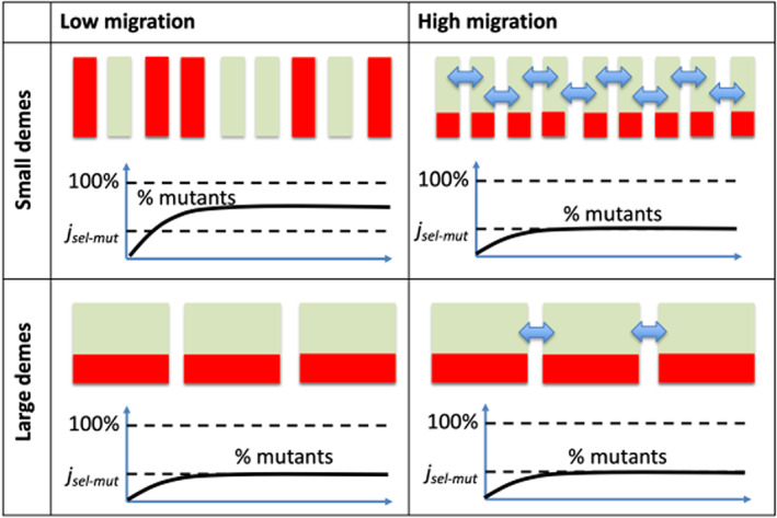
Summary of results: de novo forward and back mutation with varying migration (columns) and deme size (rows), assuming a constant total population. There are no absorbing states. Individual demes are represented as green rectangles, and the level of mutants in each is shown in red. Total frequency of mutants panels schematically show the percent of mutants as a function of time; the black dashed lines represent the selection‐mutation balance, , and 100% fixation.
3.2.3. The role of the effective population size,
The effective population size () is the number of individuals in an “idealized” (panmictic) population that would be characterized by a specified quantity (measuring the strength of genetic drift such as variance, coalescence, etc.) that is equal to that in the real population. Population fragmentation into subdivided demes can increase (Nei & Takahata, 1993; Wakeley & Takahashi, 2004) or decrease (Whitlock & Barton, 1997) the effective population size. As shown in (Nei & Takahata, 1993) (Wright‐Fisher type island model), and (Wakeley & Takahashi, 2004) (Moran type island model), in the case where the overall population structure does not change for a long evolutionary time (as is the case in our model), the effective population size of a subdivided population can be much larger than the total population size (and is larger with lower levels of migration). At the same time, the effective selection coefficient () becomes smaller. A natural question is then: is the change in and sufficient to explain the observed differences in mutant dynamics between non‐fragmented and fragmented populations, including a higher frequency of deleterious mutations?
In Appendix S2 Section 3.1, we discuss the diffusion approximation for our fragmented model with migration, and obtain the following approximations for the effective population size and effective selection coefficient:
| (13) |
| (14) |
Figure S7 illustrates the validity of the diffusion approximation and motivates the definition of the “variance” effective population size, Equation 13, see also Figure S8 that compares this approximation with numerically obtained values for .
In order to obtain the predicted average number of mutants in a fragmented system, based on the effective population size, we can apply Equation 11, where the system size is given by and mutant fitness . The results are presented in Figure S9. While the general trend is qualitatively captured (higher degrees of fragmentation result in a larger number of disadvantageous mutants), the size of the effect predicted by this substitution is not quantified correctly.
This suggests that, as noted in (Wakeley & Takahashi, 2004), it is not only a change in effective population size that distinguishes the subdivided population with many demes and migration from the singular panmictic one. In other words, a rescaling of population size (and adjusting the selection coefficient) does not make the two populations equivalent. If a fragmented population with effective population size is replaced with a well‐mixed population of size , the number of mutants will increase compared to a well‐mixed population of size . In addition, the frequency of mutants in each individual deme will be very different: a single large deme at selection‐mutation balance (well‐mixed population) versus many demes that are either completely wild type or completely mutant (fragmented population). As a consequence, the mutant dynamics in a fragmented system will proceed in a qualitatively different way, and the expected number of mutants will not be governed by a simple balance between production and selection, as it is in a panmictic system.
3.2.4. When can we expect to see more mutants than predicted by selection‐mutation balance?
The number of disadvantageous mutants is amplified relative to a well‐mixed population when the population is highly fragmented (i.e. the individual patches are sufficiently small) and the migration rate is not too high, see Figure 6.
Even in the absence of migration, if each deme size is too large, then fixation will almost never be reached and fluctuation around the selection‐mutation balance in each deme will be observed instead. On the other hand, if the deme size is very small (), then the expected number of mutants is approximately 50% of the system, as each deme will spend about 50% of the time at mutant extinction and 50% of the time at mutant fixation because of the small mutation rate (not shown). As the number of individuals per deme increases, this effect of fixation continues to elevate the number of mutants, but contributes less and less as the fixation probability decreases. Therefore, as the deme size grows, the expected number of mutants (the blue line in Figure 7) will extrapolate between two regimes: (i) the fast fixation regime, where the mean number of mutants in a deme is given by (Equation 1, green line in Figure 7) and drift dominates, and (ii) the selection‐mutation balance (Equation 2, yellow line in Figure 7) where selection dominates. To estimate the threshold deme size, , above which the expected frequency of mutants becomes close to selection‐mutation balance, we find the intersection of the fast‐fixation (green) and selection‐mutation balance (yellow) lines by solving the equation for :
| (15) |
As represents the threshold value for which drift can overpower selection if and selection (of the disadvantageous mutant) overpowers drift for , we have that can be thought of as an approximation of the “selection effective population size” for our model in the absence of migration (Gravel, 2016; Lynch, 2007; Wang et al., 2016). For more details on these calculations, see Appendix S2 Section 3. If the deme size is smaller than , a significantly larger number of mutants compared to the selection‐mutation balance is expected. However, if demes are connected to each other and migration is present, this may weaken the effect. Under intense migration, the expected number of mutants tends to that predicted by selection‐mutation balance. Therefore, an important question is: what is the level of migration that is sufficient to lower the mutant levels back to that of selection‐mutation balance?
FIGURE 7.

Estimating . The expected number of mutants in a single deme in the absence of migration is shown as a function of ; it is computed numerically (blue circles) by determining the principal eigenvector of the transition matrix, see Equation 3, and also by using approximations (8) and (10) (blue line). The green line represents the fast fixation regime (, Equation 1); the yellow line is the selection‐mutation balance, (Equation 2). The parameters are and . The threshold value is shown by the dashed vertical line.
In this model, the overall intensity of migration (monotonically) depends on several parameters (see Table 1): the probability of a migration event per update (), the number of swaps during a migration event (), and the number of individuals exchanged during a swapping event (). To simplify the discussion, we will fix two of these to and , focusing on the parameter as the one parameter determining the rate of migration.
Figure 8a demonstrates how a threshold value of the migration probability can be calculated. Fixing the values of , and , simulations were run for different choices of the deme size, , and the mean frequency of mutants (i.e. the mutant number divided by the total population size, ) was determined for each . As anticipated, the expected mutant frequencies are higher than the level predicted by the selection‐mutation balance; also, they decrease with the deme size, , and migration probability, . To quantify the migration probability that, for each , corresponds to a significant decay in the mutant population, we defined as the value of that leads the frequency of mutants to fall to twice the selection‐mutation balance. In Figure 8a, intersections of the mutant frequencies with are marked with coloured symbols and their horizontal coordinate gives . This quantity decreases with .
FIGURE 8.

The role of migration in the level of mutants. (a) the mean frequency of mutants as a function of , calculated as a temporal average over time‐steps; the bars represent the standard error. Different curves correspond to different values of . The horizontal lines are and . The parameters are , and . (b) the threshold values, , are plotted against the corresponding , for several values of . The exponent (Equation 16) is . The rest of the parameters are and .
Figure 8b shows the threshold migration rate as a function of for several different values of . We observe that the dependence is exponential, and propose the empirical law:
| (16) |
where the constants and do not depend on . The value of the exponent, , can be found by fitting (see Figure 8); it is difficult to derive analytically because it falls in the intermediate migration rate regime (where our approximations of no migration or strong migration do not apply). Therefore, we use numerical approximations to calculate it, as shown in Figure 8. Overall, Figure 8b shows that the threshold migration rate () decays exponentially with , which is the deme size divided by the threshold deme size (). This implies that even for small increases in deme size , drastic decreases in the migration rate are needed to maintain the inflated number of mutants in the fragmented population compared to the expected number of mutants at selection‐mutation balance. Section 3.2 of the Appendix S2 presents similar results obtained in the case of the Wright‐Fisher model.
4. DISCUSSION AND CONCLUSION
Divided and fragmented habitats are common in nature. Some examples are naturally occurring habitats such as islands (in the context of biogeography), aquatic habitats separated by land (such as ponds or lakes), different parts of a plant that can be inhabited by lower organisms, or hosts that are inhabited by ecto‐ and endoparasites. Human activities may lead to further fragmentation of natural environments, which has implications for conservation biology. In general, most natural habitats are spatially structured, and are likely to be characterized by demes or microdemes, with population movement between them, such as patches of high moisture or nutrient availability across a larger habitat. Given the ubiquity of fragmented and deme‐structured habitats in nature, it is important to obtain a better understanding of how such structures impact evolutionary dynamics. As mentioned in the introduction, several aspects of evolution in fragmented populations have been explored in the literature. Importantly, it has been shown that mutant fixation times can be significantly increased in deme‐structured habitats, even though the probability of mutant fixation remains unaltered. Other aspects of evolution in deme‐structured and fragmented habitats, however, remain to be explored in more detail from an evolutionary theory point of view, but also from an experimental point of view to verify model predictions. A more complete understanding of these dynamics is crucial for better understanding evolutionary processes in natural populations.
Experimentally testing the validity of evolutionary mathematical models of fragmented and deme‐structured populations can be challenging, yet is an important component of this work. We set up experiments in which murine cell colonies were grown in ninety‐six wells, with migration implemented as swapping small numbers of cells between randomly chosen wells with a pipette. We used this system to quantify the distribution of neutral mutants across the demes/wells. The experimental findings confirmed that while the mean number of mutants is not influenced by migration, the probability distribution is, consistent with theoretical predictions. We used the same model to also investigate the distribution of disadvantageous mutants across the demes, which was not feasible to follow experimentally. Furthermore, we extended the model to include de novo mutations and examined the average level at which the mutants were expected to persist, and compare this to the level that is expected due to the balance between mutation and negative selection. We showed that the mutant numbers experience an increase in frequency compared to that of the selection‐mutation balance of a non‐fragmented system. We investigated this phenomenon; using the diffusion approximation, we found that this increase cannot be simply explained by an elevation in the effective population size and a decrease in the selection coefficient, which are consequences of fragmentation. In fact, an increase in the effective population size does not capture a profound change in mutant dynamics brought about by fragmentation and expressed in a shift from selection‐mutation balance to the dynamics of intermittent mutant fixation and extinction events. In a single deme, we found that the increase (compared to the selection‐mutation level) is observed when the deme size is lower than the critical size, , given by Equation 15. In a fragmented system that consists of connected demes with a probability of migration, the increase in mutant numbers above the selection‐mutation balance can be observed in small () demes as long as the migration rate is sufficiently small. The migration rate above which the mutants approach the selection‐mutation balance decays exponentially with , see Equation 16.
4.1. Implications for evolutionary biology
This work has important implications for issues surrounding standing genetic variation in populations. Our mathematical modelling results indicate that the pool of deleterious mutants that persist in a population can be significantly higher in a deme‐structured or fragmented population compared to the predictions made by models without such population structure. This means that in many natural settings, populations will carry a larger mutational load and show greater genetic variance for fitness than expected in a panmictic population. An important factor that determines whether these effects occur is the population size within individual demes relative to the migration rate, as mentioned above. Deleterious mutants are more likely to persist at higher frequencies if the within‐deme population size is relatively small, as defined mathematically in our modelling framework.
While our model makes direct predictions about the dynamics of deleterious mutations, our results could also have implications for adaptive evolution in structured populations. This is particularly true if alleles that are mildly deleterious in current environmental conditions can become advantageous later on, when the environment changes to their favour. Such changes in the environment can arise naturally, or can be induced by xenobiotics, such as drugs, pesticides or pollutants. Resistance evolution (such as against pesticides or antibiotics) is of particular applied relevance in this respect, because resistant mutants often suffer a fitness cost in the absence of the treatment and only become advantageous once treatment is initiated. The pre‐existence of resistant mutants at the selection‐mutation balance is an important determinant of outcome in such cases and our model would predict that the presence of potential variants would be more likely in structured populations. Besides a change in environment, the higher level at which disadvantageous mutants might persist can also speed up the crossing of fitness valleys, where a first mutation can lead to a selective disadvantage, but an additional mutation results in an overall advantage.
4.2. Somatic evolutionary processes
In addition, and on a more speculative level, there are also biomedical implications of our findings, if cell populations in vivo are viewed as a kind of ecosystem in which cells evolve over time. Clonal evolution takes place within tissues as individuals age. This has been clearly documented in the haematopoietic system (Lee‐Six et al., 2018), where a variety of mutant clones with different characteristics emerge over time. These mutant clones can potentially lead to a functional deterioration of the healthy tissue, and also in the longer term to the development of malignancies. These mutants can be disadvantageous, neutral or advantageous, and can form the basis for further mutation accumulation. These evolutionary processes take place in the bone marrow, where stem cells exist in niches, with traffic between different parts of the bone marrow via the blood (Wasnik et al., 2017). There is currently no detailed data that quantifies the rate at which cell populations across the individual niches/demes communicate and the rate at which they migrate. Given the intricate anatomical structures in the haematopoietic system, and given the tendency for cells to home to their specific microenvironments (Suárez‐Álvarez et al., 2012), it is likely that cell dynamics are largely governed by local processes, with a relatively low rate at which cells move from one location to another. If this is true, then according to our model, the deme structure can influence the exact spatial genetic composition of the cell population, with mutants being dominant in some parts of the bone marrow but not others, especially for disadvantageous and neutral mutants. This in turn can have implications for bone marrow biopsies when trying to assess or monitor the clonal composition of the haematopoietic system.
4.3. Tumour evolution
Similar considerations can apply to tumours in the haematopoietic system once they have started to expand. Although tumours grow over time and we have considered the evolutionary dynamics in constant populations, tumours can be characterized by periods of slow growth or temporary stasis until further mutants are generated that allow the cells to overcome specific selective barriers. In the haematopoietic system, an example could be slowly growing/indolent cases of chronic lymphocytic leukaemia (CLL), where cells grow in spatially separated lymph nodes, the spleen, and the bone marrow. The evolution of drug‐resistant mutants is a major problem that results in the eventual failure of therapies, and the level at which resistant mutants exist before the start of treatment tends to be an important determinant of the time to disease relapse (Burger et al., 2016; Komarova et al., 2014). Mathematical models have been used to calculate the number of drug‐resistant mutants, for example in chronic lymphocytic leukaemia (Komarova et al., 2014) or chronic myeloid leukaemia (Komarova & Wodarz, 2005), and these models assumed a spatially homogeneous growing tumour cell population. If drug‐resistant mutants carry a fitness cost and are therefore disadvantageous before the start of therapy, the models analysed here indicate that the organization of cells into demes can have a significant influence on the abundance of pre‐existing mutants. Depending on the deme size and the migration rate, the number of resistant cells can be significantly larger than predicted by the selection‐mutation balance, which could dramatically speed up the rate at which the tumour relapses during therapy. If the drug‐resistant mutants are advantageous, which happens in the presence of treatment, then the spatial structure could also result in a significant effect on quantities such as the timing of mutant expansion (and therefore treatment failure). Advantageous mutant dynamics, however, are beyond the scope of this study. There are also implications for sampling strategies when attempting to assess the burden of drug‐resistant mutants before therapy such that the true genetic diversity across the different locations is determined, rather than a skewed picture arising from the analysis of one or just a few locations. This concept of optimal sampling of tumours has also been explored with spatially explicit computational models in a different context (Opasic et al., 2019; Zhao et al., 2014). Our analysis particularly highlights the need to experimentally measure the rate at which lymphocytes redistribute from one lymph node compartment to another, which would allow a more accurate prediction about how the deme structures in the haematopoietic system influence the evolution of CLL cells.
4.4. Spatial migration
Finally, we note that in our model analysis, migration is assumed to be among randomly (uniformly) chosen demes. For migration that is spatially restricted, disadvantageous mutant levels will be elevated compared to non‐spatially restricted migration because once a region of demes becomes fixed with the mutant, it is less likely that the wild type will be reintroduced (for geometric reasons). Therefore, spatially restricted migration increases population fragmentation compared to mixed migration, which increases the number of mutants. Including different spatially restricted patterns of migration could be an interesting extension of our current work.
AUTHOR CONTRIBUTIONS
J.K. developed the computational models, analysed them, ran computer simulations, and wrote the paper. D.B developed the experimental model, ran the experiments, and wrote the paper. N.L.K. developed the computational models, analysed them, ran computer simulations, and wrote the paper. D.W. developed the computational models, analysed them, ran computer simulations, and wrote the paper. J.P developed the experimental model, ran the experiments, and wrote the paper.
CONFLICT OF INTEREST
The authors have no conflict of interest to declare.
PEER REVIEW
The peer review history for this article is available at https://publons.com/publon/10.1111/jeb.14131.
Supporting information
Appendix S1.
Appendix S2.
ACKNOWLEDGEMENTS
This work was partially supported by National Science Foundation (NSF) grants NSF DMS‐1812601 and NSF GEO/OCE 1848576, National Institute for Biomedical Imaging and Bioengineering (NIBIB) grant R21EB026617, National Cancer Institute (NCI) grant U01CA265709, and by the NSF‐Simons Center for Multiscale Cell Fate Research (CMCF). The funders had no role in study design, data collection and analysis, decision to publish, or preparation of the manuscript.
Kreger, J. , Brown, D. , Komarova, N. L. , Wodarz, D. , & Pritchard, J. (2023). The role of migration in mutant dynamics in fragmented populations. Journal of Evolutionary Biology, 36, 444–460. 10.1111/jeb.14131
Endnote
Note that in this formulation we do not distinguish between a birth‐death or a death‐birth process (Kaveh et al., 2015). Assume . In a true death‐birth process, if a mutant dies, the probability of mutant division would be given by (assuming that a cell that just dies cannot divide). Similarly, in a true birth‐death process, the probability of mutant death following a mutant division would be (assuming that an individual that just divided does not immediately die). In the present model formulation we do not include these considerations.
DATA AVAILABILITY STATEMENT
The experimental data is uploaded as supplemental material and example Mathematica and C++ scripts for figures and simulations are publicly available at the following github repository: https://github.com/jessekreger/fragmented_populations.
REFERENCES
- Burger, J. A. , Landau, D. A. , Taylor‐Weiner, A. , Bozic, I. , Zhang, H. , Sarosiek, K. , Wang, L. , Stewart, C. , Fan, J. , Hoellenriegel, J. , Sivina, M. , Dubuc, A. M. , Fraser, C. , Han, Y. , Li, S. , Livak, K. J. , Zou, L. , Wan, Y. , Konoplev, S. , … Wu, C. J. (2016). Clonal evolution in patients with chronic lymphocytic leukaemia developing resistance to BTK inhibition. Nature Communications, 7(1), 1–13. [DOI] [PMC free article] [PubMed] [Google Scholar]
- Chakraborty Partha Pratim, Nemzer Louis R., and Kassen Rees. Experimental evidence that metapopulation structure can accelerate adaptive evolution. bioRxiv; preprint, July 2021. 10.1101/2021.07.13.452242 [DOI] [Google Scholar]
- Cherry, J. L. (2003). Selection in a subdivided population with local extinction and recolonization. Genetics, 164(2), 789–795. [DOI] [PMC free article] [PubMed] [Google Scholar]
- Cherry, J. L. , & Wakeley, J. (2003). A diffusion approximation for selection and drift in a subdivided population. Genetics, 163(1), 421–428. [DOI] [PMC free article] [PubMed] [Google Scholar]
- Conwill, A. , Kuan, A. C. , Damerla, R. , Poret, A. J. , Baker, J. S. , Delphine Tripp, A. , Alm, E. J. , & Lieberman, T. D. (2022). Anatomy promotes neutral coexistence of strains in the human skin microbiome. Cell Host & Microbe, 30, 171–182.e7. [DOI] [PMC free article] [PubMed] [Google Scholar]
- Earn, D. J. D. , Levin, S. A. , & Rohani, P. (2000). Coherence and conservation. Science, 290(5495), 1360–1364. https://Science.sciencemag.org/content/290/5495/1360.full.pdf [DOI] [PubMed] [Google Scholar]
- Ewens, W. J. (2007). Mathematical population genetics. In nterdisciplinary applied mathematics (Vol. 27). Springer‐Verlag. [Google Scholar]
- Fudenberg, D. , Nowak, M. A. , Taylor, C. , & Imhof, L. A. (2006). Evolutionary game dynamics in finite populations with strong selection and weak mutation. Theoretical Population Biology, 70(3), 352–363. [DOI] [PMC free article] [PubMed] [Google Scholar]
- Fung, C. , Tan, S. , Nakajima, M. , Skoog, E. C. , Camarillo‐Guerrero, L. F. , Klein, J. A. , Lawley, T. D. , Solnick, J. V. , Fukami, T. , & Amieva, M. R. (2019). High‐resolution mapping reveals that microniches in the gastric glands control helicobacter pylori colonization of the stomach. PLoS Biology, 17(5), e3000231. [DOI] [PMC free article] [PubMed] [Google Scholar]
- Fusco, D. , Gralka, M. , Kayser, J. , Anderson, A. , & Hallatschek, O. (2016). Excess of mutational jackpot events in expanding populations revealed by spatial Luria–Delbrück experiments. Nature Communications, 7, 12760. [DOI] [PMC free article] [PubMed] [Google Scholar]
- Gravel, S. (2016). When is selection effective? Genetics, 203(1), 451–462. [DOI] [PMC free article] [PubMed] [Google Scholar]
- Hanski, I. (1998). Metapopulation dynamics. Nature, 396(6706), 41–49. [Google Scholar]
- Hanski, I. , & Gilpin, M. (1991). Metapopulation dynamics: Brief history and conceptual domain. Biological Journal of the Linnean Society, 42(1–2), 3–16. [Google Scholar]
- Hauert, C. , & Imhof, L. A. (2012). Evolutionary games in deme structured, finite populations. Journal of Theoretical Biology, 299, 106–112. [DOI] [PubMed] [Google Scholar]
- Kalarus, K. , & Nowicki, P. (2015). How do landscape structure, management and habitat quality drive the colonization of habitat patches by the dryad butterfly (Lepidoptera: Satyrinae) in fragmented grassland? PLoS One, 10(9), e0138557. [DOI] [PMC free article] [PubMed] [Google Scholar]
- Kareiva, P. , Mullen, A. , & Southwood, R. (1990). Population dynamics in spatially complex environments: Theory and data. Philosophical Transactions of the Royal Society of London. Series B: Biological Sciences, 330(1257), 175–190. [Google Scholar]
- Karlin, S. , & McGregor, J. (1962). On a genetics model of Moran. Mathematical Proceedings of the Cambridge Philosophical Society, 58(2), 299–311. [Google Scholar]
- Kaveh, K. , Komarova, N. L. , & Kohandel, M. (2015). The duality of spatial death‐birth and birth‐death processes and limitations of the isothermal theorem. Royal Society Open Science, 2(4), 140465. [DOI] [PMC free article] [PubMed] [Google Scholar]
- Kerr, B. , Neuhauser, C. , Bohannan, B. J. M. , & Dean, A. M. (2006). Local migration promotes competitive restraint in a host–pathogen ‘tragedy of the commons. Nature, 442, 75–78. [DOI] [PubMed] [Google Scholar]
- Kimura, M. (1962). On the probability of fixation of mutant genes in a population. Genetics, 47(6), 713–719. [DOI] [PMC free article] [PubMed] [Google Scholar]
- Komarova, N. L. , Burger, J. A. , & Wodarz, D. (2014). Evolution of ibrutinib resistance in chronic lymphocytic leukemia (CLL). Proceedings of the National Academy of Sciences of the United States of America, 111(38), 13906–13911. [DOI] [PMC free article] [PubMed] [Google Scholar]
- Komarova, N. L. , & Wodarz, D. (2005). Drug resistance in cancer: Principles of emergence and prevention. Proceedings of the National Academy of Sciences of the United States of America, 102(27), 9714–9719. [DOI] [PMC free article] [PubMed] [Google Scholar]
- Lander, T. A. , Harris, S. A. , Cremona, P. J. , & Boshier, D. H. (2019). Impact of habitat loss and fragmentation on reproduction, dispersal and species persistence for an endangered Chilean tree. Conservation Genetics, 20(5), 973–985. [Google Scholar]
- Lavigne, C. , Reboud, X. , Lefranc, M. , Porcher, E. , Roux, F. , Olivieri, I. , & Godelle, B. (2001). Evolution of genetic diversity in metapopulations: Arabidopsis thaliana as an experimental model. Genetics Selection Evolution, 33(Suppl 1), S399–S423. [Google Scholar]
- Lee‐Six, H. , Øbro, N. F. , Shepherd, M. S. , Grossmann, S. , Dawson, K. , Belmonte, M. , Osborne, R. J. , Huntly, B. J. P. , Martincorena, I. , Anderson, E. , O’Neill, L. , Stratton, M. R. , Laurenti, E. , Green, A. R. , Kent, D. G. , & Campbell, P. J. (2018). Population dynamics of normal human blood inferred from somatic mutations. Nature, 561(7724), 473–478. [DOI] [PMC free article] [PubMed] [Google Scholar]
- Levin, S. A. (1974). Dispersion and population interactions. The American Naturalist, 108(960), 207–228. [Google Scholar]
- Levin, S. A. , & Powell, T. M. (1993). Lecture notes in biomathematics. In Patch dynamics (Vol. 96). Springer‐Verlag. [Google Scholar]
- Levins, R. (1969). Some demographic and genetic consequences of environmental heterogeneity for biological Control1. Bulletin of the Entomological Society of America, 15(3), 237–240. https://academic.oup.com/ae/article‐pdf/15/3/237/18805526/besa15‐0237.pdf [Google Scholar]
- Loewe, L. , & Hill, W. G. (2010). The population genetics of mutations: Good, bad and indifferent. Philosophical Transactions of the Royal Society of London. Series B: Biological Sciences, 365(1544), 1153–1167. [DOI] [PMC free article] [PubMed] [Google Scholar]
- López‐Cortegano, E. , Pouso, R. , Labrador, A. , Pérez‐Figueroa, A. , Fernández, J. , & Caballero, A. (2019). Optimal management of genetic diversity in subdivided populations. Frontiers in Genetics, 10, 843. [DOI] [PMC free article] [PubMed] [Google Scholar]
- Lynch, M. (2007). The origins of genome architecture. Oxford University Press. [Google Scholar]
- Lynch, M. , Conery, J. , & Burger, R. (1995). Mutation accumulation and the extinction of small populations. The American Naturalist, 146(4), 489–518. [Google Scholar]
- Lynch, M. , & Gabriel, W. (1990). Mutation load and the survival of small populations. Evolution, 44(7), 1725–1737. [DOI] [PubMed] [Google Scholar]
- Maruyama, T. (1970). On the fixation probability of mutant genes in a subdivided population. Genetical Research, 15(2), 221–225. [DOI] [PubMed] [Google Scholar]
- Maruyama, T. (1974). A simple proof that certain quantities are independent of the geographical structure of population. Theoretical Population Biology, 5(2), 148–154. [DOI] [PubMed] [Google Scholar]
- Michael, C. (2004). Whitlock and Reinhard Bürger. Fixation of new mutations in small populations. In Couvet D., Ferrière R., & Dieckmann U. (Eds.), Evolutionary conservation biology, Cambridge studies in adaptive dynamics (pp. 155–170). Cambridge University Press. [Google Scholar]
- Moran, P. A. P. (1958). Random processes in genetics. Mathematical Proceedings of the Cambridge Philosophical Society, 54(1), 60–71. [Google Scholar]
- Moran, P. A. P. (1962). The statistical processes of evolutionary theory. Clarendon Press. [Google Scholar]
- Nei, M. , & Takahata, N. (1993). Effective population size, genetic diversity, and coalescence time in subdivided populations. Journal of Molecular Evolution, 37(3), 240–244. [DOI] [PubMed] [Google Scholar]
- Opasic, L. , Zhou, D. , Werner, B. , Dingli, D. , & Traulsen, A. (2019). How many samples are needed to infer truly clonal mutations from heterogenous tumours? BMC Cancer, 19(1), 1–11. [DOI] [PMC free article] [PubMed] [Google Scholar]
- Patwa, Z. , & Wahl, L. M. (2008). The fixation probability of beneficial mutations. Journal of the Royal Society, Interface, 5(28), 1279–1289. [DOI] [PMC free article] [PubMed] [Google Scholar]
- Prugh, L. R. , Hodges, K. E. , Sinclair, A. R. E. , & Brashares, J. S. (2008). Effect of habitat area and isolation on fragmented animal populations. Proceedings of the National Academy of Sciences of the United States of America, 105(52), 20770–20775. [DOI] [PMC free article] [PubMed] [Google Scholar]
- Rochat, E. , Manel, S. , Deschamps‐Cottin, M. , Widmer, I. , & Joost, S. (2017). Persistence of butterfly populations in fragmented habitats along urban density gradients: Motility helps. Heredity, 119(5), 328–338. [DOI] [PMC free article] [PubMed] [Google Scholar]
- Rubinoff, D. , & Powell, J. A. (2004). Conservation of fragmented small populations: Endemic species persistence on California's smallest channel Island. Biodiversity and Conservation, 13(13), 2537–2550. [Google Scholar]
- Slatkin, M. (1977). Gene flow and genetic drift in a species subject to frequent local extinctions. Theoretical Population Biology, 12(3), 253–262. [DOI] [PubMed] [Google Scholar]
- Slatkin, M. (1981). Fixation probabilities and fixation times in a subdivided population. Evolution; International Journal of Organic Evolution, 35(3), 477–488. [DOI] [PubMed] [Google Scholar]
- Suárez‐Álvarez, B. , López‐Vázquez, A. , & López‐Larrea, C. (2012). Mobilization and homing of hematopoietic stem cells. Stem Cell Transplantation, 741, 152–170. [DOI] [PubMed] [Google Scholar]
- Thomas, J. A. , Bourn, N. A. , Clarke, R. T. , Stewart, K. E. , Simcox, D. J. , Pearman, G. S. , Curtis, R. , & Goodger, B. (2001). The quality and isolation of habitat patches both determine where butterflies persist in fragmented landscapes. Proceedings of the Royal Society. Series B: Biological Sciences, 268(1478), 1791–1796. [DOI] [PMC free article] [PubMed] [Google Scholar]
- Wade, M. J. , & McCauley, D. E. (1988). Extinction and recolonization: Their effects on the genetic differentiation of local populations. Evolution; International Journal of Organic Evolution, 42(5), 995–1005. [DOI] [PubMed] [Google Scholar]
- Wakeley, J. (2003). Polymorphism and divergence for Island‐model species. Genetics, 163(1), 411–420. [DOI] [PMC free article] [PubMed] [Google Scholar]
- Wakeley, J. , & Takahashi, T. (2004). The many‐demes limit for selection and drift in a subdivided population. Theoretical Population Biology, 66(2), 83–91. [DOI] [PubMed] [Google Scholar]
- Wang, J. , Santiago, E. , & Caballero, A. (2016). Prediction and estimation of effective population size. Heredity, 117(4), 193–206. [DOI] [PMC free article] [PubMed] [Google Scholar]
- Wasnik, S. , Chen, W. , Ahmed, A. S. I. , Zhang, X.‐B. , Tang, X. , & Baylink, D. J. (2017). Chapter 5 ‐ hsc niche: Regulation of mobilization and homing. In Vishwakarma A. & Karp J. M. (Eds.), Biology and engineering of stem cell niches (pp. 63–73). Academic Press. [Google Scholar]
- Whitlock, M. C. , & Barton, N. H. (1997). The effective size of a subdivided population. Genetics, 146(1), 427–441. [DOI] [PMC free article] [PubMed] [Google Scholar]
- Whitlock, M. C. (2003). Fixation probability and time in subdivided populations. Genetics, 164(2), 767–779. [DOI] [PMC free article] [PubMed] [Google Scholar]
- Willi, Y. , Griffin, P. , & Van Buskirk, J. (2013). Drift load in populations of small size and low density. Heredity, 110(3), 296–302. [DOI] [PMC free article] [PubMed] [Google Scholar]
- Wright, S. (1931). Evolution in Mendelian populations. Genetics, 16(2), 97–159. [DOI] [PMC free article] [PubMed] [Google Scholar]
- Zhao, B. , Pritchard, J. R. , Lauffenburger, D. A. , & Hemann, M. T. (2014). Addressing genetic tumor heterogeneity through computationally predictive combination therapy. Cancer Discovery, 4(2), 166–174. https://cancerdiscovery.aacrjournals.org/content/4/2/166.full.pdf [DOI] [PMC free article] [PubMed] [Google Scholar]
Associated Data
This section collects any data citations, data availability statements, or supplementary materials included in this article.
Supplementary Materials
Appendix S1.
Appendix S2.
Data Availability Statement
The experimental data is uploaded as supplemental material and example Mathematica and C++ scripts for figures and simulations are publicly available at the following github repository: https://github.com/jessekreger/fragmented_populations.