

1. Introduction
Diffusion-weighted imaging (DWI) has been investigated for the last two decades to detect, grade, and stage tumors across the body, e.g. [1–3], as a complementary or even an alternative method to invasive biopsies [4]. For example, since biopsy of the renal medulla is quite rare due to safety concerns [5], imaging might play a strong alternative role. Recently, the Intravoxel-incoherent motion (IVIM)-DWI technique [6] has been of more interest because of its potential to separate relatively substantial kidney flow effects from microstructural parameter estimates from diffusion and give additional insight into the tubular and vascular flow. Several recent reviews [7–9] have summarized works exploring IVIM-DWI in recent years to assess renal kidney function, acute kidney injury, chronic kidney diseases, and kidney tumors.
Most DWI acquisitions use an Echo-planar imaging (EPI) readout which, while rapid and insensitive to intershot motional phase errors, is prone to artifacts caused by eddy currents, and static field inhomogeneity [10], as well as requiring some form of respiratory motion mitigation. There are multiple solutions to treat each of these (as reviewed recently [11]), such as using bipolar gradients to minimize eddy current effects [7], using FSL TOPUP [12] to correct for magnetic field inhomogeneity using images acquired at forward and reverse phase encoding directions, and prospective triggering or retrospective registration for motion mitigation. Kidney motion quantification has also been a subject of interest in radiotherapy in pursuit of optimizing dose delivery, e.g. [13, 14], where maximal craniocaudal kidney movements of around 10–16 mm have been measured with regard to the breathing phase.
Several recent studies demonstrate motion dependence of field inhomogeneity in different body organs and correct it either retrospectively or prospectively (e.g. [15–18]). Vannesjo et al. [15] have profiled field maps of the cervical spine during breathing. For this purpose, they considered different scenarios of breath-hold (expired and inspired) and free-breathing (deep and normal) and tracked respiratory motion using respiratory sensors during the acquisition while acquiring field maps. Since their work has focused on the cervical spine, they have reduced the dimension of the profiles to only one dimension, i.e. the craniocaudal direction. Additionally, they used online motion shimming as a prospective method to correct this artifact. Hutter et al. [19] allowed more arbitrary ordering of diffusion encoding in successively acquired slices, in combination with a second reversed phase encoded image, to improve motion and distortion correction of brain DWI in the setting of fetal imaging. Andersson et.al. [20] took subject rotation into account when applying distortion correction using a field map for brain DWI.
In the case of renal imaging, Coll-Font et al. [16] have retrospectively corrected magnetic field inhomogeneity distortion of renal DW-MRI acquiring near-simultaneous forward and reverse images of the same diffusion encoding with time lags of 30–50 ms allowing for correction of each image with its respective reversed phase encoding at approximately the same breathing phase and directional diffusion encoding assuming there is insignificant breathing motion within this time gap. Similar methods have been used to correct for motion dependence of magnetic inhomogeneity in the brain [17, 18]. Reversed phase encoding has also been employed for distortion correction of kidney DWI in other recent studies [21, 22]. Coll-Font et al. [16] discuss minor out-of-phase movement of the two kidneys which is probably caused by cardiac motion. The out-of-phase movement of the right and left kidneys has also been considered in [23] where their kidney MR processing flowchart recommends separate motion correction for the right and left kidneys. More recently, it has been shown that diffusion weighted image quality is dependent on the kidney laterality [24]. This could be caused by a number of confounding factors, one of which might be this out-of-phase movement.
In the present work, we first corrected for motion in each kidney separately similar to the approach of [23]. Second, we introduced an alternative method to [16] for correction of magnetic field inhomogeneity for DTI sets which only required the acquisition of 32 forward and 32 reversed b-value=0 images to sample breathing-phase-dependent motion in the kidneys and determine B0 field distortion correction separately for different breathing phases. Additionally, similar to the approach of [15] for the cervical spine, we demonstrated field inhomogeneity variations in the kidneys with regard to the breathing phase and kidney region.
2. Methods
2.1. Image acquisition
In this HIPAA-compliant and IRB-approved prospective study, 8 volunteers (6M, ages 28–51) provided written informed consent and had abdominal imaging performed in a 3 T MRI system (MAGNETOM Prisma; Siemens Healthcare, Erlangen, Germany) in supine position with posterior spine array and anterior body array RF coils and chest leads for ECG gating. Coronal oblique T2-weighted SSFSE (HASTE) images (TR/TE=1000/91 ms, flip angle 120 degrees, matrix 320/320/20, resolution 1.1/1.1/5 mm) were collected for anatomical reference. Sagittal phase-contrast (PC) MRI images through the left renal artery were collected at multiple cardiac phases to estimate systolic and diastolic phases for kidney tissue (TR/TE=32.82/3.56 ms, flip angle 26 degrees, matrix 198/256/1, resolution 1.6/1.6/10 mm, 24–27 phases, velocity encoding 80 mm/s). With a prototype advanced diffusion-weighted imaging sequence with dynamic field correction [25], cardiac triggered at either systolic (N=8) or diastolic (N=8) phase oblique coronal DWI (TR/TE 2800/81 ms, matrix 192/192/1, resolution 2.2/2.2/5 mm) were collected at 10 b-values (b=0, 10, 30, 50, 80, 120, 200, 400, 600, 800 s/mm2) and (for b>0 images) 12 diffusion sensitizing directions, with twice refocused spin echo bipolar diffusion gradients. Multiple b-values were collected consistent with ongoing studies of advanced renal DWI contrast, though only DTI analysis was performed in the present work. Additionally, to correct for field inhomogeneity, 32 right-to-left and 32 left-to-right phase-encoding direction b=0 images were acquired in systolic phase, half of which were acquired before the DTI acquisition and the other half afterward to account for any possible bulk motion during the DTI acquisition.
2.2. Field inhomogeneity correction based on breathing phase binning
FSL TOPUP [12] is widely used for the correction of field inhomogeneity induced distortions. Diffusion-weighted images with the same encoding are acquired with opposite phase encoding directions and supplied as an input to TOPUP to find the field map inhomogeneity coefficients which are later used to correct the whole DTI data set.
Fig. 1 shows a brief flowchart and diagram of registration and application of TOPUP correction on the diffusion-weighted sets. In this study, the 32 forward and 32 reverse phase-encoding b=0 images randomly sampled kidney motion with regards to the breathing phase. The 64 images were registered to one of the forward b=0 images in the set taken as reference using the freely available software package FireVoxel, build 380, https://firevoxel.org/. Mutual information metric and 2D rigid transformation were used starting from initial positions on the regular transformation grid and further optimized using the Nelder-Mead simplex method [26]. These registration settings are consistent both with the single acquired slice and the known motion pattern of kidneys predominantly in the oblique plane defined by their long and short axes. FireVoxel outputs the whole rigid transform matrix, from which the craniocaudal translation element was logged and used to create 1 mm craniocaudal motion bins using an in-house-developed code written in MATLAB and Statistics Toolbox (Release 2022a, The MathWorks, Inc., Natick, Massachusetts, United States). Each of these bins included at least four forward and reverse phase encoding pairs. The images ascribed to each of these motion bins were supplied to TOPUP to create field maps. The procedure was repeated for registrations based on the right and left kidneys separately, using a manually prescribed mask of the kidney alone to focus the registration procedure.
Figure 1.
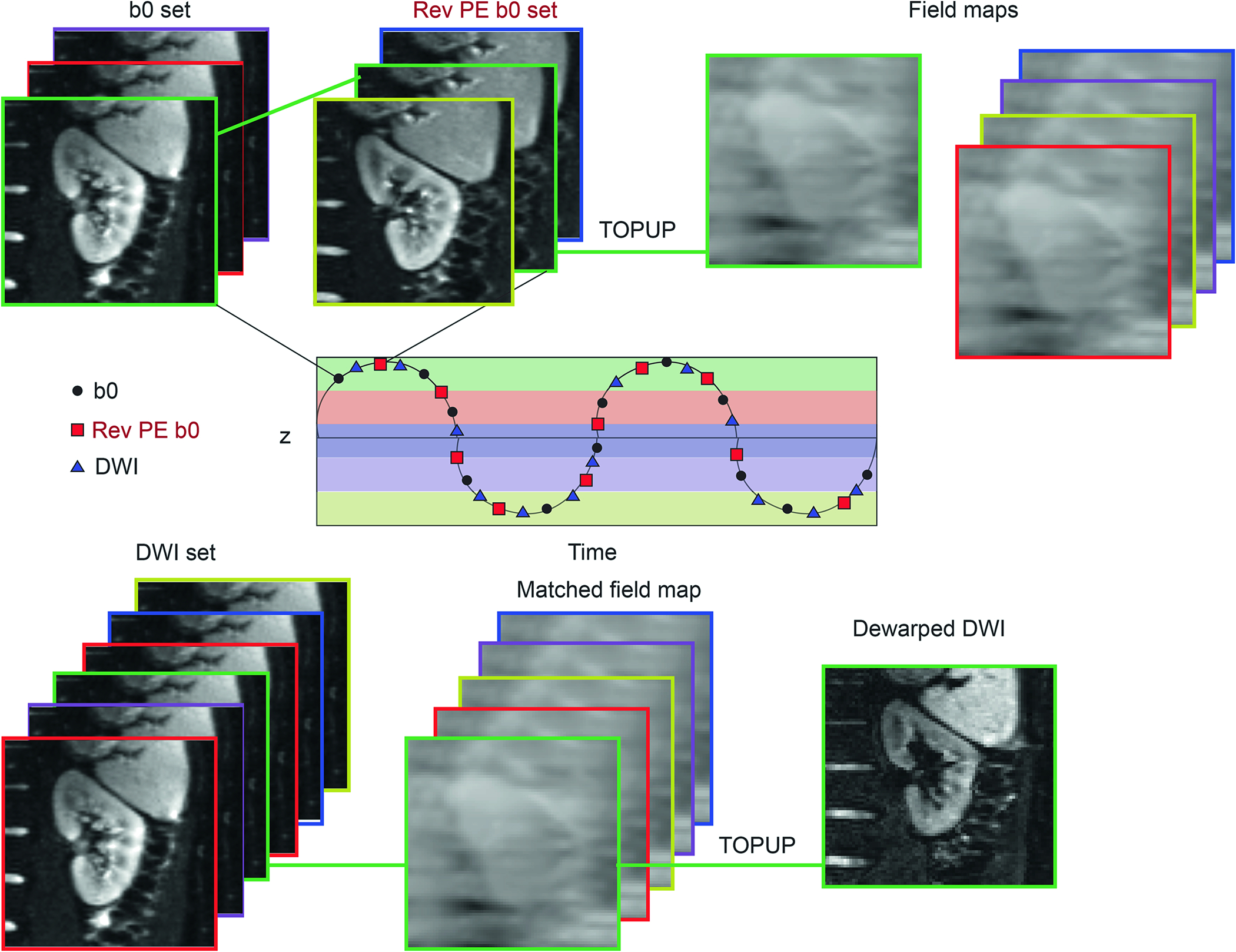
The diagram for the proposed workflow including registration, motion binning, and TOPUP application. A pair of b = 0 image sets with forward and reversed phase encoding are collected over the respiratory cycle and registered to the reference position (z=0) with a rigid body 2D algorithm, and the craniocaudal coordinate of this registration assigned them to position bins (color-coded above). Pairs of forward and reverse b0 images from the same bin were then submitted to the TOPUP algorithm to determine the field inhomogeneity maps for each bin. A full DWI stack was then also self-registered, assigned to position bins, and then dewarped by the appropriate field inhomogeneity map for that bin.
Each image in the DTI sets (systolic or diastolic gated) was separately registered to the reference b=0 image of the subject. Accordingly, each of the images were ascribed to one of the motion bins using the craniocaudal displacement coordinate of each for the application of field inhomogeneity correction. While sampling the complete breathing phase pattern was not always possible using the 32 forward and reverse images alone, they covered more than 95% of images from different DTI sets. In case a DTI image was acquired at a breathing phase greater or smaller than the maximum or minimum bin, they were corrected using the maximum or minimum bin, respectively. Parametric maps of DTI metrics mean diffusivity (MD) and fractional anisotropy (FA) were calculated from a range of the acquired b-values (200 < b < 800 s/mm2) for each acquisition using custom code developed in MATLAB.
For comparison, a TOPUP correction without respiratory phase resolution (one-bin TOPUP) was performed as follows. First, all forward phase encoding b=0 images were registered together, and similarly for the reversed phase encoding b=0 set, each of these stacks were averaged to produce one pair of forward and reverse b=0 images that were used to generate a single field map. All images of a DWI acquisition were co-registered and dewarped using this single field map for the one-bin motion correction strategy.
Field maps derived for the kidneys were investigated further as a function of three parameters: a) kidney laterality (i.e. right and left), b) four coarse manually segmented kidney regions (i.e. apical, upper, middle, and lower [27, 28]), and c) breathing phase. Uncorrected, one-bin motion TOPUP corrected, and multi-binned motion TOPUP corrected images from the full DTI image set for 5 subjects underwent a 2D rigid registration to their corresponding HASTE slice. These registration settings are consistent both with the single acquired slice and the known motion pattern of kidneys predominantly in the oblique plane defined by their long and short axes. A mutual information metric of this registration was generated using Firevoxel software for each image. This comparison was used to evaluate if TOPUP correction improves morphology restoration.
To further demonstrate how motion binning improves the quality of the DWI dataset, several lines of view cutting through the apical region of the kidneys parallel to the L-R phase encoding direction were drawn for each subject separately for each side. These lines were used to compare the TOPUP corrections with and without considering the motion. For each line the following equation was used to measure the center of the image at each DWI slice:
where was the signal intensity, and were the start and end point of the lines. The standard deviation of the center of lines across each DWI set was used as a measure of TOPUP correction.
Cortex and medulla regions of interest were segmented manually on b0 and FA maps, respectively, for each kidney case, and used to measure mean MD and FA values from maps generated from DWI series originating from each of the three correction methods no correction (N), one-bin correction (O), and multi-bin correction (M). Cortex ROIs were a single cortical stripe while medullary ROIs sampled at least three pyramids (upper, middle, and lower pole). Separate ROIs were drawn on uncorrected and corrected image sets due to their differing morphology.
2.3. Statistical analysis
Mixed model analysis of variance was used to assess the effect of phase, region and side on field inhomogeneity (denoted FI) averaged over corresponding ROIs. FI was the dependent variable and the model to predict FI included phase, region and side as fixed classification factors and the anonymized subject ID as a random classification factor. Phase was included as a classification factor rather than a numeric factor to avoid an assumption of a linear association between FI and phase. The correlation structure induced by the inclusion of multiple dependent variable observations per subject was modeled by assuming results to be symmetrically correlated when associated with the same subject and independent when associated with different subjects. Tests for significant variation with each factor in this model were quantified by an F statistic and p-value. Results are summarized in terms of the mean ± standard deviation (SD) of FI and the least squares (LS) mean ± standard error (SE) of the LS mean at each level of a given factor, where the LS mean at a given level of a selected factor represents an estimate of the mean FI to be expected for a random subject with that level of the selected factor. Regarding the mutual information metric of registration of DWI to anatomical HASTE images, the multiple DWI (b-values, directions) per subject were treated as a blocking factor in the analysis to account for the fact that mutual information is expected to change over the blocks. Mixed model analysis of variance was used to assess the effect of each DWI (hereafter referred to as block), side and method (denoted N (No correction), O (one bin correction), and M (multi-bin correction) on mutual information (denoted MI). MI was the dependent variable and the model to predict MI included side, block and method as fixed classification factors and an anonymized subject ID as a random classification factor. The correlation structure induced by the inclusion of multiple MI observations per subject was modeled by assuming results to be symmetrically correlated when associated with the same subject and independent when associated with different subjects. Results are summarized in terms of the mean ± standard deviation (SD) of MI of a given factor. MI metrics from different TOPUP methods (N, O, and M) were compared via t-statistics of pairwise comparisons for all acquired images. Statistical tests for FI and MI metrics were conducted at the two-sided 5% significance level using SAS version 9.4 software (SAS Institute, Cary, NC).
For the line profile analysis, all line profile standard deviations for a given subject, kidney, and correction method (O or M) were averaged and compared with a paired sample t-test (Matlab software) between correction methods. DTI metrics MD and FA were compared between the three correction methods (N, O, and M) and cardiac phases (systole and diastole) via paired sample t-tests. Values in cortex vs. medulla for each phase and method were compared via independent samples t-tests. These comparisons were performed using SPSS Statistics software (IBM Corp., v. 26.0.1.1).
3. Results
One of the subjects had excessive out of slice motion and was removed from all future analysis. For two of the subjects, a convergence issue of TOPUP was observed because the kidney slice of interest had significant sampling of spinal cord cerebrospinal fluid (CSF), involving sufficiently large changes in magnetic field to confound the TOPUP algorithm and induce large shifts of nearby renal tissue. These subjects did not contribute FI values from the apical region to the analysis. Overall, seven subjects contributed to FI derivations for the lower, middle and upper regions and five subjects contributed to FI derivations for the apical layer. Regarding the respiratory phase binning, 3 bins were used for 2 kidneys, 4 bins for 3 kidneys, 5 bins for 3 kidneys, and 6 bins for 2 kidneys.
3.1. Field inhomogeneity
Figure 2a corresponds to one-bin distortion correction (O) and shows motion-dependent FI maps of one subject, highlighting lateral and regional dependence of field inhomogeneity. Figure 2b corresponds to multi-bin distortion correction (M) and shows additional dependence of the field map on breathing phase. In the mixed model analysis of variance of field inhomogeneity, FI was found to vary significantly (p<0.001) with each factor considered (Region: F = 294.36; Side: F = 61.32; Phase: F = 4.5). The following results describe values and comparisons for each of these factors individually. Figure 2c shows the histograms of the same two kidneys for the respective breathing phases of figure 2b, showing the evolution of field map from inhalation to exhalation.
Figure 2.

Example field inhomogeneity maps in left and right kidneys for (a) one bin correction (O) and (b) for multi-bin correction (M) throughout breathing cycle showing clear dependencies on kidney side, region, and respiratory phase. The respective field map histograms of (b) are shown in (c).
Fig. 3a is a boxplot of field inhomogeneity vs. kidney side (KS), including all breathing phases and kidney regions. The average field inhomogeneity was 103.6±82.3 and 66.9±74.9Hz in the left and right kidneys, respectively (p-value=0.00043). Table 1 summarizes global mean and LS mean values stratified by kidney side. The LS mean difference ± standard error of the LS mean difference between the left and right kidneys (left minus right) was 45.5 ± 5.9. This difference was significant (p<0.001) implying that mean FI was significantly higher for the left kidney than for the right kidney. Table 2 summarizes global mean and LS mean values stratified by kidney region. The LS mean monotonically increased from the lower to the apical region. Fig. 3b is a boxplot of field inhomogeneity vs. kidney region for each kidney including all breathing phases. Fig 4 shows plots of field map inhomogeneity vs. breathing phase for the apical region of the left and right kidney, and the lower region of the left and right kidney of each subject.
Figure 3.

Group boxplot of field inhomogeneity vs. kidney laterality or side (KS), including all breathing phases and kidney regions (a). Group boxplot of field inhomogeneity vs. kidney region for each kidney including all breathing phases (b).
Table 1.
The observed mean and standard deviation (SD) of FI for the left and right kidneys and the LS mean and standard error (SE) of the LS mean for the left and right kidneys. N is the number of observations for the indicated kidney.
| Kidney | N | Mean | SD | LS Mean | SE |
|---|---|---|---|---|---|
| Left | 121 | 104 | 82 | 115 | 6 |
| Right | 118 | 67 | 75 | 68 | 6 |
Table 2.
The observed mean and standard deviation (SD) of field inhomogeneity (FI) within each region and the LS mean and standard error (SE) of the LS mean within each region. N is the number of observations for the indicated region.
| Region | N | Mean | SD | LS Mean | SE |
|---|---|---|---|---|---|
| Lower | 65 | 28 | 54 | 26 | 5 |
| Middle | 65 | 45 | 67 | 46 | 5 |
| Upper | 65 | 119 | 49 | 120 | 5 |
| Apical | 44 | 184 | 51 | 196 | 6 |
Figure 4.

The plot of field map inhomogeneity vs. breathing phase for the apical region of the left (a) and right (b) kidney, and the lower region of the left (c) and right (d) kidney of each color coded subject.
3.2. Mutual information registration performance
In the mixed model analysis of variance of mutual information, MI was found to vary significantly (p<0.001) with consideration of factors kidney side: F=374.9 and correction method: F=574.4. The results in Tables 3 and 4 indicate that the mean of MI was significantly lower for no correction than for each of the corrected methods (O and M) on each side and over both sides combined (p<0.001 for all comparisons). Additionally, MI was significantly lower for O than M in the left kidney (p<0.001), whereas, MI difference for the two methods was not significant in the right kidney (p=0.86).
Table 3.
The mean and standard deviation (SD) of mutual information (MI) from DWI=HASTE registration on the left and right sides and over both sides together.
| Multi-bin | No correction | One bin | ||||
|---|---|---|---|---|---|---|
| Side | Mean | SD | Mean | SD | Mean | SD |
| Right | 1.40 | 0.06 | 1.39 | 0.06 | 1.40 | 0.06 |
| Left | 1.39 | 0.06 | 1.37 | 0.06 | 1.39 | 0.06 |
| Both | 1.39 | 0.06 | 1.38 | 0.06 | 1.39 | 0.06 |
Table 4.
The t statistic and p-value for the pairwise comparison of methods (N: No correction; O: One-bin TOPUP; M: Multi-bin TOPUP) on the left and right side and over both sides combined.
| Methods Compared | Overall | Right Side | Left Side | ||||
|---|---|---|---|---|---|---|---|
| T | P Value | T | P Value | T | P Value | ||
| M | N | 23.82 | <0.001 | 24.45 | <0.001 | 28.85 | <0.001 |
| M | O | −0.21 | 0.835 | −0.17 | 0.864 | 3.52 | <0.001 |
| N | O | −24.02 | <0.001 | −24.63 | <0.001 | −25.32 | <0.001 |
In the line profile analysis, multi-binning resulted in significantly better registration of the images in the phase encoding dimension especially in the apical region when quantified by the standard deviation of the center of movement lines cutting through the kidneys in each DWI image (0.0724 with multi-bin vs. 0.0885 mm with one bin, p=0.006).
Fig. 5 shows DTI parametric maps of an example case where TOPUP correction with motion binning performed better than without motion binning. Fig. 6 a and b qualitatively show the improved temporal registration of a sample DTI dataset for the case M vs. O via 1D line profiles through the apex of a kidney from right to left (i.e. the distortion correction direction). Additionally, purple lines are plotted horizontally at the same locations for M and O to demonstrate the better performance of M compared to O. Figure 6c shows the evolution of the centroid of these line profiles over a full DTI acquisition for the two methods, showing a smaller range of variation for the multi-bin correction algorithm. As seen both in the spatial extent of the profiles and their 1st moment (figure 6c), the motion binning reduces the spatiotemporal variability of the registered, dewarped stack.
Figure 5.
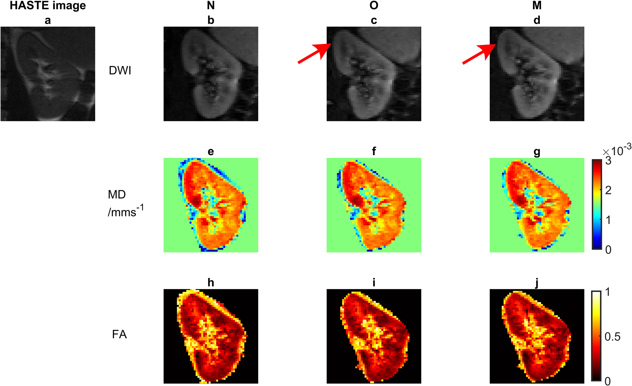
An example case showing improved TOPUP correction with motion binning. a) HASTE image, a sample diffusion-weighted image with b) no TOPUP correction (N), c) TOPUP correction without motion binning (O), d) TOPUP correction with motion binning (M), the MD maps corresponding to e) b, f) c, and g) d, the FA maps corresponding to h) b, i) c, and j) d. The arrows indicate bending of the images at the top and more similarity with the HASTE image.
Figure 6.

A sample set of line profiles along the phase encode direction (i.e. right to left) to illustrate improved temporal registration after TOPUP correction of multiple motion bins (M) (a) vs. the one bin case (O) (b). Temporal tracking of the center of images from the same DWI set with increasing image number to compare motion binning and one bin TOPUP correction (c). Note, (a), (b), and (c) have the same abscissa labelling image number in a sample DTI set. The purple lines are at the same location for (a) and (b) for ease of comparison.
3.3. DTI metrics
Table 5 shows mean and standard deviation of FA and MD values in cortex and medulla for diastolic and systolic cardiac phases and for the three correction methods (N, O, M) in this study. Regarding method comparison, significant FA differences were found in cortex between M and O in diastole, and significant MD differences were found in cortex between O and N and between M and N in systole and diastole. In medulla, no significant differences were found between any pair of methods for either systole or diastole. Regarding cardiac phase dependence, a significant difference was found between systole and diastole for FA in cortex with no correction (N). Finally, regarding tissue comparison, FA was significantly different between cortex and medulla for all phases and methods, while MD was only significantly different between cortex and medulla for diastole with no correction.
Table 5.
Mean (standard deviation) values of fractional anisotropy (FA) in cortex and medulla for each cardiac phase (systolic or diastolic) and distortion correction method (M:multi-bin TOPUP, O:one-bin TOPUP, N: no correction). Statistical differences are labelled.
| Correction method | |||||
|---|---|---|---|---|---|
| Parameter | Tissue | Phase | M | O | N |
| FA | Cortex | Systolic | 0.22 (0.01)4 | 0.23 (0.02)4 | 0.23 (0.04)1,4 |
| Diastolic | 0.21 (0.04)3,4 | 0.20 (0.04)3,4 | 0.21 (0.04)1,4 | ||
| Medulla | Systolic | 0.33 (0.04)4 | 0.32 (0.05)4 | 0.34 (0.03)4 | |
| Diastolic | 0.33 (0.03)4 | 0.32 (0.05)4 | 0.34 (0.03)4 | ||
| MD | Cortex | Systolic | 2.01 (0.22)2 | 2.01 (0.21)2 | 2.06 (0.18)2 |
| Diastolic | 1.96 (0.20)2 | 1.96 (0.18)2 | 2.04 (0.10)2,4 | ||
| Medulla | Systolic | 1.94 (0.23) | 1.95 (0.24) | 1.98 (0.19) | |
| Diastolic | 1.92 (0.13) | 1.92 (0.14) | 1.93 (0.13)4 | ||
Significant difference between diastolic and systolic FA in case of no correction
Significant difference between MD of one and multi-bin correction vs. no correction for the cortex
Significant difference between diastolic FA of multi-bin vs. one bin for the cortex
Significant difference between cortex and medulla.
4. Discussion
In general, if EPI images are corrected for field inhomogeneity, organ morphology is improved. This would enable the radiologists to more easily sample the same ROIs across different imaging modalities (e.g. BOLD, DCE, CT) and compare them. The results of this study have shown improvements in this morphologic accuracy can be obtained with motion-resolved distortion correction.
The results of this study indicate significant dependence of field inhomogeneity on kidney side, region, and breathing phase. It has been recently emphasized that magnetic field inhomogeneity is not a local phenomenon and high distortion in one area affects other areas in the image/body which might have uniform magnetic fields [29]. Accordingly, these dependencies can be understood by considering the overall susceptibility of the body to the magnetic field in the craniocaudal direction and the relative distance of the kidneys from the lungs, spleen, stomach, spinal cord or liver at different breathing phases.
Consistent with recent studies [16, 21, 22], results also indicate better morphologic accuracy following correction of distortion diffusion-weighted EPI images induced by this inhomogeneity. We have observed that this correction performs better when performed in a respiratory-resolved fashion (i.e. multi-bin TOPUP) for the left kidney. Also, we observe in a focused line profile analysis a benefit in reduced spatial variability within a given acquisition when the multi-bin algorithm is performed. Finally, regarding DTI metrics derived from the kidney, to first order the trends of tissue and phase dependencies are recapitulated by all methods employed, consistent with findings of other recent studies [16, 21, 22]. However, with more scrutiny some differences exist between corrected and uncorrected DTI metrics, mostly indicating slightly reduced cortical MD values with correction. These results indicate that if correction methods such as the respiratory resolved TOPUP applied in this study are used, that comparison with literature values without correction should be done with caution.
Kidney microstructure is in general less explored from the MR microstructural perspective compared to some other organs, in part due to its own acquisition challenges (motion, distortion). The principal aim of the study was to correct motion-dependent field inhomogeneity in the kidneys as one of the most important artifacts. However, there was a secondary goal to demonstrate and characterize breathing phase-dependent field inhomogeneity. This perspective might have application to the context of imaging of the kidney at the more challenging platform of 7 T in the future, and analogous to works such as [15, 30] on spinal cord MRI at 7 T, inform similar solutions such as online shimming.
Some limitations exist in this study. First, two of the subjects were excluded from this study because their respective slice had intercepted a significant pool of cerebrospinal fluid (CSF), resulting in the apical region of the kidneys undergoing dramatic displacement. Similarly, Lim et al. [21] observed similar artifacts that required some degree of masking before performing TOPUP field map derivation. Since that study employed head to feet phase encoding, their masking focused upon the stomach organ. Out of slice motion exceeding one slice thickness also was limiting for one case which was not correctable with the current single slice paradigm. These artifacts could be the subject of future studies to either modify TOPUP convergence methods or introduce methods that combine TOPUP with machine learning to distinguish CSF, stomach, and kidney morphology. Another limitation is that the current protocol collects a single slice within the TR of 2800 ms, for purposes of maintaining a consistent cardiac cycle, which involves a considerable dead time in the acquisition. In principle this interval could be used for collecting reference b=0 images rather than in a separate acquisition, analogous to the efficient double-echo acquisition shown by Coll-Font et.al. [16]. Future work may explore such a modification. Additionally, if one forgoes cardiac gating to save acquisition time, extension of the FI correction method developed in this study to multislice imaging would be feasible.
Also, while for most cases motion binning improved field inhomogeneity correction, there were cases where using a universal field map coefficient gave better results. This may originate from the higher SNR achieved by averaging all of the 32 forward and reverse phase encoded images together. This may thus be a tradeoff between the need to quantify motion-dependent distortion and the need for sufficient signal averages to determine the field map confidently. In the apical areas, the motion dependence predominates, while in basal regions more signal averages are more beneficial than motion mapping.
In conclusion, we have demonstrated a workflow for motion-resolved distortion correction of kidney DWI using a combination of free-breathing acquisition, reversed phase encoding distortion correction, and retrospective registration. This module of image processing is expected to enhance the quality and application of quantitative DWI in pathologic populations (e.g. chronic kidney disease, allografts, and renal masses) in the future.
5. Acknowledgements
This work was supported by the National Institutes of Health (NIH) (R01CA245671).
Footnotes
Nima Gilani: Methodology, Software, Writing and editing
Artem Mikheev: FireVoxel software development and support.
Inge M. Brinkmann and Thomas Benkert: Siemens pulse sequence development and installation
Dibash Basukala: Methodology, Editing
James S. Babb: Statistics
Malika Kumbella: Research coordination and subject recruitment
Hersh Chandarana: Clinical application, Writing and editing, Supervision, Securing funding
Eric E. Sigmund: Conceptualization, Writing and editing, Supervision, Securing funding
Publisher's Disclaimer: This is a PDF file of an unedited manuscript that has been accepted for publication. As a service to our customers we are providing this early version of the manuscript. The manuscript will undergo copyediting, typesetting, and review of the resulting proof before it is published in its final form. Please note that during the production process errors may be discovered which could affect the content, and all legal disclaimers that apply to the journal pertain.
References
- 1.Kim S, Naik M, Sigmund E, and Taouli B, Diffusion-weighted MR imaging of the kidneys and the urinary tract. Magn Reson Imaging Clin N Am, 2008. 16(4): p. 585–96. [DOI] [PubMed] [Google Scholar]
- 2.Squillaci E, Manenti G, Di Stefano F, Miano R, Strigari L, and Simonetti G, Diffusion-weighted MR imaging in the evaluation of renal tumours. J Exp Clin Cancer Res, 2004. 23(1): p. 39–45. [PubMed] [Google Scholar]
- 3.Paudyal B, Paudyal P, Tsushima Y, Oriuchi N, et al. , The role of the ADC value in the characterisation of renal carcinoma by diffusion-weighted MRI. Br J Radiol, 2010. 83(988): p. 336–43. [DOI] [PMC free article] [PubMed] [Google Scholar]
- 4.Cornelis F, Tricaud E, Lasserre AS, Petitpierre F, et al. , Routinely performed multiparametric magnetic resonance imaging helps to differentiate common subtypes of renal tumours. Eur Radiol, 2014. 24(5): p. 1068–80. [DOI] [PubMed] [Google Scholar]
- 5.Lees GE, Cianciolo RE, and Clubb FJ Jr., Renal biopsy and pathologic evaluation of glomerular disease. Top Companion Anim Med, 2011. 26(3): p. 143–53. [DOI] [PubMed] [Google Scholar]
- 6.Le Bihan D, Breton E, Lallemand D, Grenier P, Cabanis E, and Laval-Jeantet M, MR imaging of intravoxel incoherent motions: application to diffusion and perfusion in neurologic disorders. Radiology, 1986. 161(2): p. 401–7. [DOI] [PubMed] [Google Scholar]
- 7.Zhang JL and Lee VS, Renal perfusion imaging by MRI. J Magn Reson Imaging, 2020. 52(2): p. 369–379. [DOI] [PubMed] [Google Scholar]
- 8.Caroli A, Schneider M, Friedli I, Ljimani A, et al. , Diffusion-weighted magnetic resonance imaging to assess diffuse renal pathology: a systematic review and statement paper. Nephrol Dial Transplant, 2018. 33(suppl_2): p. ii29–ii40. [DOI] [PMC free article] [PubMed] [Google Scholar]
- 9.Ljimani A, Caroli A, Laustsen C, Francis S, et al. , Consensus-based technical recommendations for clinical translation of renal diffusion-weighted MRI. MAGMA, 2020. 33(1): p. 177–195. [DOI] [PMC free article] [PubMed] [Google Scholar]
- 10.Pierpaoli C, Artifacts in diffusion MRI. Diffusion MRI: theory, methods and applications, 2010: p. 303–318. [Google Scholar]
- 11.Haskell MW, Nielsen JF, and Noll DC, Off-resonance artifact correction for MRI: A review. NMR in Biomedicine, 2022: p. e4867. [DOI] [PMC free article] [PubMed] [Google Scholar]
- 12.Smith SM, Jenkinson M, Woolrich MW, Beckmann CF, et al. , Advances in functional and structural MR image analysis and implementation as FSL. Neuroimage, 2004. 23 Suppl 1: p. S208–19. [DOI] [PubMed] [Google Scholar]
- 13.Hallman JL, Mori S, Sharp GC, Lu HM, Hong TS, and Chen GT, A four-dimensional computed tomography analysis of multiorgan abdominal motion. Int J Radiat Oncol Biol Phys, 2012. 83(1): p. 435–41. [DOI] [PubMed] [Google Scholar]
- 14.Bussels B, Goethals L, Feron M, Bielen D, et al. , Respiration-induced movement of the upper abdominal organs: a pitfall for the three-dimensional conformal radiation treatment of pancreatic cancer. Radiother Oncol, 2003. 68(1): p. 69–74. [DOI] [PubMed] [Google Scholar]
- 15.Vannesjo SJ, Miller KL, Clare S, and Tracey I, Spatiotemporal characterization of breathing-induced B0 field fluctuations in the cervical spinal cord at 7T. Neuroimage, 2018. 167: p. 191–202. [DOI] [PMC free article] [PubMed] [Google Scholar]
- 16.Coll-Font J, Afacan O, Hoge S, Garg H, et al. , Retrospective Distortion and Motion Correction for Free-Breathing DW-MRI of the Kidneys Using Dual-Echo EPI and Slice-to-Volume Registration. J Magn Reson Imaging, 2021. 53(5): p. 1432–1443. [DOI] [PMC free article] [PubMed] [Google Scholar]
- 17.Afacan O, Hoge WS, Wallace TE, Gholipour A, Kurugol S, and Warfield SK, Simultaneous Motion and Distortion Correction Using Dual-Echo Diffusion-Weighted MRI. J Neuroimaging, 2020. 30(3): p. 276–285. [DOI] [PMC free article] [PubMed] [Google Scholar]
- 18.Gallichan D, Andersson JL, Jenkinson M, Robson MD, and Miller KL, Reducing distortions in diffusion-weighted echo planar imaging with a dual-echo blip-reversed sequence. Magn Reson Med, 2010. 64(2): p. 382–90. [DOI] [PubMed] [Google Scholar]
- 19.Hutter J, Christiaens DJ, Schneider T, Cordero-Grande L, et al. , Slice-level diffusion encoding for motion and distortion correction. Medical Image Analysis, 2018. 48: p. 214–229. [DOI] [PMC free article] [PubMed] [Google Scholar]
- 20.Andersson JLR, Graham MS, Drobnjak I, Zhang H, and Campbell J, Susceptibility-induced distortion that varies due to motion: Correction in diffusion MR without acquiring additional data. NeuroImage, 2018. 171: p. 277–295. [DOI] [PMC free article] [PubMed] [Google Scholar]
- 21.Lim RP, Lim JC, Teruel JR, Botterill E, et al. , Geometric Distortion Correction of Renal Diffusion Tensor Imaging Using the Reversed Gradient Method. J Comput Assist Tomogr, 2021. 45(2): p. 218–223. [DOI] [PMC free article] [PubMed] [Google Scholar]
- 22.Borrelli P, Cavaliere C, Basso L, Soricelli A, Salvatore M, and Aiello M, Diffusion Tensor Imaging of the Kidney: Design and Evaluation of a Reliable Processing Pipeline. Sci Rep, 2019. 9(1): p. 12789. [DOI] [PMC free article] [PubMed] [Google Scholar]
- 23.Li LP, Leidner AS, Wilt E, Mikheev A, et al. , Radiomics-Based Image Phenotyping of Kidney Apparent Diffusion Coefficient Maps: Preliminary Feasibility & Efficacy. J Clin Med, 2022. 11(7). [DOI] [PMC free article] [PubMed] [Google Scholar]
- 24.McTavish S, Van AT, Peeters JM, Weiss K, et al. , Motion compensated renal diffusion weighted imaging. Magn Reson Med, 2022. [DOI] [PubMed] [Google Scholar]
- 25.Haneda J, Hagiwara A, Hori M, Wada A, et al. , A Comparison of Techniques for Correcting Eddy-current and Motion-induced Distortions in Diffusion-weighted Echo-planar Images. Magn Reson Med Sci, 2019. 18(4): p. 272–275. [DOI] [PMC free article] [PubMed] [Google Scholar]
- 26.Nelder JA and Mead R, A Simplex-Method for Function Minimization. Computer Journal, 1965. 7(4): p. 308–313. [Google Scholar]
- 27.Bonsib SM, Renal anatomy and histology. The Heptinstall’s pathology of the kidney, 2007: p. 8. [Google Scholar]
- 28.Graves FT, The anatomy of the intrarenal arteries and its application to segmental resection of the kidney. Br J Surg, 1954. 42(172): p. 132–9. [DOI] [PubMed] [Google Scholar]
- 29.Begnoche JP, Schilling KG, Boyd BD, Cai LY, Taylor WD, and Landman BA, EPI susceptibility correction introduces significant differences far from local areas of high distortion. Magn Reson Imaging, 2022. 92: p. 1–9. [DOI] [PMC free article] [PubMed] [Google Scholar]
- 30.Vannesjo SJ, Clare S, Kasper L, Tracey I, and Miller KL, A method for correcting breathing-induced field fluctuations in T2*-weighted spinal cord imaging using a respiratory trace. Magn Reson Med, 2019. 81(6): p. 3745–3753. [DOI] [PMC free article] [PubMed] [Google Scholar]