A mathematical model to assess the impact of testing and isolation compliance on the transmission of COVID-19

Abstract

The COVID-19 pandemic has ravaged global health and national economies worldwide. Testing and isolation are effective control strategies to mitigate the transmission of COVID-19, especially in the early stage of the disease outbreak. In this paper, we develop a deterministic model to investigate the impact of testing and compliance with isolation on the transmission of COVID-19. We derive the control reproduction number ${\mathcal{R}}_C$, which gives the threshold for disease elimination or prevalence. Using data from New York State in the early stage of the disease outbreak, we estimate ${\mathcal{R}}_C=7.989$. Both elasticity and sensitivity analyses show that testing and compliance with isolation are significant in reducing ${\mathcal{R}}_C$ and disease prevalence. Simulation reveals that only high testing volume combined with a large proportion of individuals complying with isolation have great impact on mitigating the transmission. The testing starting date is also crucial: the earlier testing is implemented, the more impact it has on reducing the infection. The results obtained here would also be helpful in developing guidelines of early control strategies for pandemics similar to COVID-19.

Highlights

• •We build a model to study the impact of testing and isolation compliance on the spread of COVID-19 in the early stage.
• •We carry out the stability analysis for equilibria and sensitivity analysis for the control reproduction number.
• •Parameter values for transmission and disease-induced death rates are derived via data fitting.
• •Our results suggest that testing and isolation compliance are important, but other control measures are also needed.
• •The daily infection peak implies that high testing rates with high isolation compliance can notably reduce the prevalence.

1. Introduction

The SARS-CoV-2 pandemic, which started in late 2019, has ravaged global health and national economies worldwide (Jackson, 2021). The virus causing this pandemic belongs to the family of coronaviruses, which can cause respiratory illness in humans (Cleveland Clinic, (Accessed Mar 1, 2022). Current evidence suggests that the main route of transmission of the SARS-CoV-2 virus is from person to person via small liquid droplets when an infected person coughs, sneezes or breathes, particularly in poorly ventilated or crowded indoor settings (Cleveland Clinic, (Accessed Mar 1, 2022). The pandemic is currently ongoing despite control measures (e.g, vaccination, social distancing). To date, there have been over 500 million cases of COVID-19 globally, with about 6 million deaths (Worldometer, (Accessed June 6, 2022). The United States (US) alone has recorded over 90 million COVID-19 cases, with over a million deaths from the COVID-19 disease (Worldometer, (Accessed June 6, 2022). New York (NY) state is among several US states with high mortality and infection rates. Specifically, NY has recorded nearly 6 million cases with over 70,000 deaths thus far (Worldometer, (Accessed July 18, 2022A). In this paper, using data from New York State in an early phase of the pandemic, we adopt a deterministic model to investigate the impact of testing and compliance with isolation orders on the transmission of COVID-19.

Mass testing is an effort to test the general population to detect infectious individuals, including those who remain asymptomatic (Shen et al., 2021). It is cost-effective (López Seguí et al., 2021), detects new infections rapidly, and provides an accurate picture of spread within regions by capturing asymptomatic and symptomatic cases (Shen et al., 2021). Tests for COVID-19 were developed expeditiously, with the US Food and Drug Administration (FDA) issuing an Emergency Use Authorization for the real-time polymerase chain reaction (RT-PCR) test on February 4, 2020 (CDC, (Accessed June 14, 2022), and for the first point of care antigen test on May 9, 2020 (Hahn & Shuren, 2020-05-09). However, a sufficient supply of COVID-19 testing materials was not readily available in the US early in the pandemic (Cohen, 2020). Manufacturing errors in February 2020 led to a massive shortage of tests in the US in the early spring of 2020 (Cohen, 2020). Partly for these reasons, it was not realistic to implement mass testing in the early months of the pandemic. In the US, testing was at first reserved for very specific situations (only symptomatic individuals with history of travel to Wuhan, China, or those exposed to a known COVID-19 positive individual), and gradually increased throughout the spring and summer of 2020 (Patel et al., 2020). The US was unable to ramp up to even 1 million tests per day until October 2020 (Center for Systems Science and Engineering at Johns Hopkins University, 2020). Even that number of tests is not sufficient to truly implement mass testing. Further, understanding the effects of testing becomes even more relevant as we now know that a large proportion of COVID-19 infections (around 40–45%) are asymptomatic (Oran & Topol, 2020; Seibold et al., 2022). Clearly, most asymptomatic individuals (those without known COVID-19 positive contacts) would not have met the stringent criteria for testing early in the pandemic. Since these individuals were not being tested, they would have had no indication that they needed to isolate themselves. On the other hand, studies have indicated that asymptomatic individuals are infectious (Oran & Topol, 2020) and may be a substantial driver of disease spread (Johansson et al., 2021). This raises one of the questions we examine in our model: If it had been possible to implement mass testing of both symptomatic and asymptomatic individuals during spring and summer 2020, what effect could such testing have had on the course of the pandemic? Testing alone, however, cannot serve as a control measure. That is, the testing itself does not have an effect on the number of individuals infected. The behavior of individuals after testing is the key factor for disease control. Testing allows the determination of which individuals should be isolated. The isolation serves as the control measure, preventing disease spread by prohibiting contact with others. However, even when isolation is required by law or encouraged by compensation, perfect isolation is not achievable (Bodas, Peleg, & 6, 2020; Patel et al., 2021; Tseng et al., 2021). There will be individuals who refuse to comply with isolation orders, as well as mistakes in attempting to isolate. This raises the second question we address in our model: how does isolation compliance affect the spread of COVID-19 disease? The interplay between the testing level of asymptomatic cases and compliance with isolation regulations is what we seek to elucidate with our model.

Mathematical modeling has frequently been used to describe the dynamics of infectious and non-infectious diseases. To date, several types of mathematical and statistical models, including ordinary differential equation (ODE) models and agent-based models (ABMs), have been used to study and forecast the dynamics of the COVID-19 pandemic in the US and worldwide. In this paper, we use a deterministic compartmental ODE model to explicitly consider the effects of asymptomatic spread and compliance with isolation orders on the spread of COVID-19 disease. We next review some key models in relation to our proposed model. This short review includes models that predict and address issues of testing, isolation, physical distancing, and compliance, which were vital in controlling the epidemic at its early stages before the availability of vaccines.

Several authors have previously used compartmental mathematical models to investigate the role of testing and isolation on the spread of COVID-19 (Aronna et al., 2021; Bartha et al., 2021; Bhaduri et al., 2022; Howerton et al., 2021; Leontitsis et al., 2021; Sturniolo et al., 2021). In particular, Sturniolo et al. (Sturniolo et al., 2021) presented a compartmental ODE model investigating the effects of testing, contact tracing, and isolation. Unlike our model, the model in (Sturniolo et al., 2021) assumes perfect compliance with isolation orders, and instead of considering asymptomatic individuals, includes an exposed but not yet infectious class. The authors of (Sturniolo et al., 2021) are less concerned with predicting specific disease dynamics than with comparing the results of their method of including contact tracing in a compartmental model to results from agent-based models. In (Bartha et al., 2021), Bartha et al. proposed a compartmental ODE model that considers only symptom-based testing, using the assumption that adjusting the probability of showing symptoms adequately accounts for asymptomatic individuals. Bhaduri et al. (Bhaduri et al., 2022) presented a model looking at testing without explicitly including asymptomatic individuals or a measure of compliance with isolation measures. The model analyzed in (Bhaduri et al., 2022), mostly focuses on finding the effects of false negative test results on spread of COVID-19. Aronna et al. (Aronna et al., 2021) developed a compartmental ODE model accounting for testing and isolation strategies while separating out asymptomatic individuals. In contrast to our model, however, the model formulation in (Aronna et al., 2021) assumes a constant population size and does not include vital dynamics. Another compartmental model examining testing strategies while ignoring vital dynamics was presented by Leontitsis et al. (Leontitsis et al., 2021). Using stochastic, rather than deterministic, techniques, Howerton et al. (Howerton et al., 2021) used a compartmental model to examine how mass testing and isolation can augment other strategies for COVID-19 control. Additionally, a review of the types and usefulness of various compartmental models in predicting COVID-19 spread was conducted by Padmanabhan et al. (Padmanabhan et al., 2021). The effects of testing, isolation, and compliance have also been examined in the context of ABMs, as in (Almagor & Picascia, 2020; Kim & Koo, 2021; Moghadas et al., 2020; Álvarez & Rojas-Galeano, 2020). In particular, Moghadas et al. (Moghadas et al., 2020) suggested that mass testing of the asymptomatic individuals is necessary to mitigate the spread of COVID-19; this helps slow the disease spread and thus bring the pandemic under control.

Focusing on only mitigation strategies available early in the pandemic (including testing, isolation, and compliance with government policies), we develop a deterministic model that investigates the impact of mass testing of both asymptomatic and symptomatic individuals, together with compliance with isolation policies on the spread of COVID-19 disease. Our model is parameterized using historic COVID-19 transmission data from New York State for March 11th, 2020 through June 9th, 2020. In the next section, we present the model formulation, followed by model analysis in Section 3. Numerical simulations of the model are presented in Section 4 followed by a discussion in Section 5. Proofs of theorems are given in.Appendices A, B and C.

2. Model formulation

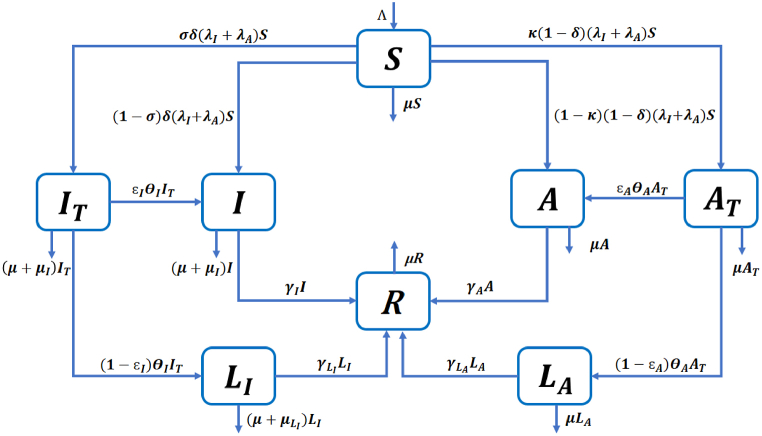
We formulate a deterministic model to study the impact of testing and isolation on the epidemic dynamics of COVID-19. The population is divided into 8 compartments, namely susceptible individuals (S), symptomatic infected individuals waiting for COVID-19 test results (I_T), symptomatic infected individuals who have not been tested or who are tested positive but are not isolated (I), isolated symptomatic infected individuals (L_I), asymptomatic infected individuals waiting for test results (A_T), asymptomatic infected individuals who have not been tested or who have tested positive but are not isolated (A), isolated asymptomatic infected individuals (L_A), and recovered individuals (R). We split symptomatic individuals into two compartments (I_T and I), and do the same for asymptomatic individuals (A_T and A), so that it is convenient to study the impact of the testing and isolation proportions on the spread of COVID-19.

We assume that all newborns and those entering the population are susceptible and enter the compartment S with recruitment rate Λ. Furthermore, all individuals die of natural causes at a constant rate μ. According to (He et al., 2020; Subramanian et al., 2021), asymptomatic infected individuals contribute substantially to the transmission of COVID-19. Therefore, we assume that susceptible individuals become infected by symptomatic infected individuals (I_T or I) with force of infection λ_I depending on the transmission rate β_I, or by asymptomatic infected individuals (A_T or A) with force of infection λ_A depending on the transmission rate β_A. A proportion δ of the new infections are symptomatic, among which a proportion σ are tested. A proportion 1 − δ of the new infections are asymptomatic, among which a proportion κ are tested. Symptomatic infected individuals waiting for their test results leave the compartment I_T at a rate θ_I, among which a proportion ϵ_I do not isolate themselves and move to the compartment I. The rest move to the isolation compartment L_I at rate (1 − ϵ_I)θ_I or die due to natural causes or COVID-19 at rates μ and μ_I, respectively. Similarly, asymptomatic infected individuals waiting for their test results leave the compartment A_T at a rate θ_A, among which a proportion ϵ_A do not isolate themselves and move to the compartment A. The rest move to the isolation compartment L_A at rate, (1 − ϵ_A)θ_A or die due to natural causes at rate μ. Infected individuals in classes I, L_I, A, and L_A recover at rates γ_I, ${\gamma }_{L_I}$, γ_A, ${\gamma }_{L_A}$, respectively. In addition, symptomatic infected individuals in classes I_T, I and L_I die due to the disease at rates μ_I, μ_I and ${\mu }_{L_I}$, respectively. In contrast, asymptomatic individuals do not die from the disease. We assume that all the parameters are positive, and that the parameters denoting proportions δ, σ, κ, ϵ_I, ϵ_A ∈ (0, 1).

Since we are focusing on an early period of COVID-19 from March 11th, 2020 to June 9th, 2020, we do not consider reinfection or vaccination in our model. Additionally, we assume that testing is perfect, i.e., no false positive or false negative results. We also assume that isolation is perfect, i.e., isolated people do not transmit the disease. Detailed descriptions of the variables and parameters are given in Table 1 and Table 2, respectively.

Table 1.

Description of variables in model (2.1).

Variable	Description
S	Susceptible individuals
IT	Symptomatic infected individuals who have been tested, waiting for results
I	Symptomatic infected individuals who have not been tested or
	who have tested positive but are not isolated
AT	Asymptomatic infected individuals who have been tested, waiting for results
A	Asymptomatic infected individuals who have not been tested or
	who have tested positive but are not isolated
LI	Isolated symptomatic infected individuals
LA	Isolated asymptomatic infected individuals
R	Recovered individuals

Table 2.

Description of parameters in model (2.1).

Parameter	Description
Λ	Recruitment rate
μ	Natural death rate
βI	Transmission rate for symptomatic individuals
βA	Transmission rate for asymptomatic individuals
δ	Proportion of symptomatic individuals among infections
σ	Proportion of tested individuals among symptomatic infections
κ	Proportion of tested individuals among asymptomatic infections
μI	Disease-induced death rate for symptomatic individuals who are not isolated
${\mu }_{L_I}$	Disease-induced death rate for symptomatic individuals who are isolated
θI	Waiting rate for symptomatic individuals
θA	Waiting rate for asymptomatic individuals
ϵI	Proportion of symptomatic individuals who do not comply with isolation order
ϵA	Proportion of asymptomatic individuals who do not comply with isolation order
γI	Recovery rate for symptomatic individuals who are not isolated
${\gamma }_{L_I}$	Recovery rate for symptomatic individuals who are isolated
γA	Recovery rate for asymptomatic individuals who are not isolated
${\gamma }_{L_A}$	Recovery rate for asymptomatic individuals who are isolated

The resulting model is described by a system of ordinary differential equations given in (2.1), with the corresponding flow diagram shown in Fig. 1

$$\left\{\begin{array}{cc}& \dot{S}(t)=\mathrm{\Lambda }-\mu S-({\lambda }_I+{\lambda }_A)S\\ & {\dot{I}}_T(t)=\sigma \delta ({\lambda }_I+{\lambda }_A)S-(\mu +{\mu }_I+{\theta }_I)I_T\\ & \dot{I}(t)=(1-\sigma )\delta ({\lambda }_I+{\lambda }_A)S+{ϵ}_I{\theta }_I{I}_T-(\mu +{\mu }_I+{\gamma }_I)I\\ & {\dot{A}}_T(t)=\kappa (1-\delta )({\lambda }_I+{\lambda }_A)S-(\mu +{\theta }_A)A_T\\ & \dot{A}(t)=(1-\kappa )(1-\delta )({\lambda }_I+{\lambda }_A)S+{ϵ}_A{\theta }_A{A}_T-(\mu +{\gamma }_A)A\\ & {\dot{L}}_I(t)=(1-{ϵ}_I){\theta }_I{I}_T-(\mu +{\mu }_{L_I}+{\gamma }_{L_I})L_I\\ & {\dot{L}}_A(t)=(1-{ϵ}_A){\theta }_A{A}_T-(\mu +{\gamma }_{L_A})L_A\\ & \dot{R}(t)={\gamma }_{I}I+{\gamma }_{A}A+{\gamma }_{L_I}{L}_I+{\gamma }_{L_A}{L}_A-\mu R\end{array}\right)$$ (2.1)

where the force of infection λ_I and λ_A are given by

$${\lambda }_I=\frac{{\beta }_I(I_T+I)}{N-L_I-L_A}\text{and}{\lambda }_A=\frac{{\beta }_A(A_T+A)}{N-L_I-L_A}.$$

Fig. 1.

Flow diagram describing COVID-19 transmission in model (2.1).

We let D(t) be the total number of individuals who die from COVID-19 in the time span of our study. It follows from model (2.1) that the equation of the rate of change of D(t) is given by

$$\dot{D}(t)={\mu }_I(I+I_T)+{\mu }_{L_I}{L}_I$$ (2.2)

Solutions with non-negative initial conditions stay in the closed positive hyperspace, ${\overline{\mathfrak{R}}}_{+}^8$, for the rest of the time, i.e. $(S,I_T,I,A_T,A,L_I,L_A,R)\in {\overline{\mathfrak{R}}}_{+}^8$, since

$$\begin{array}{cc}& \dot{S}{|}_{S=0}\ge 0,{\dot{I}}_T{|}_{I_T=0}\ge 0,\dot{I}{|}_{I=0}\ge 0,{\dot{A}}_T{|}_{A_T=0}\ge 0,\\ & \dot{A}{|}_{A=0}\ge 0,{\dot{L}}_I{|}_{L_I=0}\ge 0,{\dot{L}}_A{|}_{L_A=0}\ge 0,\dot{R}{|}_{R=0}\ge 0.\end{array}$$ (2.3)

Setting N(t) as the total population, i.e. N(t) = S(t) + I_T(t) + I(t) + A_T(t) + A(t) + L_I(t) + L_A(t) + R(t), and taking the sum of equations in (2.1), we have

$$\dot{N}(t)=\mathrm{\Lambda }-\mu N-{\mu }_I(I_T+I)-{\mu }_{L_I}{L}_I\le \mathrm{\Lambda }-\mu N,$$

where I_T ≥ 1, I ≥ 0, and L_I ≥. It follows that

$$\underset{t\to \infty }{\mathrm{lim\; sup}}N(t)\le \frac{\mathrm{\Lambda }}{\mu }.$$

We define the domain of system (2.1) to be

$$\mathrm{\Omega }=\left\{(S,I_T,I,A_T,A,L_I,L_A,R)\in {\overline{\mathfrak{R}}}_{+}^8|0\le S+I_T+I+A_T+A+L_I+L_A+R\le \frac{\mathrm{\Lambda }}{\mu }\right\}.$$

The inequalities in (2.3) imply the region Ω is positively invariant for system (2.1). We take the initial conditions in Ω, then the trajectory will stay in Ω for all time. Using a standard method (see, e.g. (Gao et al., 2021)), we can show that for any initial conditions in Ω, there exists a unique solution of system (2.1) in Ω for t ∈ [0, ∞). Therefore, system (2.1) is both epidemiologically and mathematically well posed.

3. Analysis

3.1. Control reproduction number

System (2.1) always has a disease-free equilibrium $E^0=(\frac{\mathrm{\Lambda }}{\mu },0,0,0,0,0,0,0)$. Using the next-generation matrix approach (van den Driessche & Watmough, 2002) (see Appendix A), the control reproduction number ${\mathcal{R}}_C$ is given by

$${\mathcal{R}}_C=\sigma \delta {\mathcal{R}}_{C,I_T}+(1-\sigma )\delta {\mathcal{R}}_{C,I}+\kappa (1-\delta ){\mathcal{R}}_{C,A_T}+(1-\kappa )(1-\delta ){\mathcal{R}}_{C,A},$$ (3.1)

where

$${\mathcal{R}}_{C,I_T}=\frac{{\beta }_I}{\mu +{\mu }_I+{\theta }_I}+\frac{{\beta }_I{ϵ}_I{\theta }_I}{(\mu +{\mu }_I+{\theta }_I)(\mu +{\mu }_I+{\gamma }_I)},{\mathcal{R}}_{C,I}=\frac{{\beta }_I}{\mu +{\mu }_I+{\gamma }_I},{\mathcal{R}}_{C,A_T}=\frac{{\beta }_A}{\mu +{\theta }_A}+\frac{{\beta }_A{ϵ}_A{\theta }_A}{(\mu +{\theta }_A)(\mu +{\gamma }_A)},{\mathcal{R}}_{C,A}=\frac{{\beta }_A}{\mu +{\gamma }_A}\cdot$$ (3.2)

We denote the control reproduction number associated with symptomatic and asymptomatic individuals by $\widetilde{{\mathcal{R}}_I}$ and $\widetilde{{\mathcal{R}}_A}$ respectively, that is ${\mathcal{R}}_C=\widetilde{{\mathcal{R}}_I}+\widetilde{{\mathcal{R}}_A}$, where

$$\widetilde{{\mathcal{R}}_I}=\sigma \delta {\mathcal{R}}_{C,I_T}+(1-\sigma )\delta {\mathcal{R}}_{C,I},\widetilde{{\mathcal{R}}_A}=\kappa (1-\delta ){\mathcal{R}}_{C,A_T}+(1-\kappa )(1-\delta ){\mathcal{R}}_{C,A}.$$

To see the biological interpretation of ${\mathcal{R}}_{C,I_T}$, in the incidence term $\frac{{\beta }_I{I}_{T}S}{N-L_I-L_A}$, we assume that all individuals not in the isolation classes (active population) are susceptible $(\frac{S}{N-L_I-L_A}=1)$. Then β_I represents the number of secondary infections per unit of time generated by one symptomatic infected individual who has been tested in a population with all active individuals susceptible. Here $\frac{1}{\mu +{\mu }_I+{\theta }_I}$ is the average time a symptomatic infected individual who has been tested spends in the I_T class. Therefore, $\frac{{\beta }_I}{\mu +{\mu }_I+{\theta }_I}$ represents the number of secondary infections generated by this infectious individual when in compartment I_T. After receiving the test result, this individual may not be isolated but then move to compartment I with probability $\frac{{ϵ}_I{\theta }_I}{\mu +{\mu }_I+{\theta }_I}$. For a symptomatic individual, the average time spent in compartment I is $\frac{1}{\mu +{\mu }_I+{\gamma }_I}$. Thus, the second term in the expression for ${\mathcal{R}}_{C,I_T}$ represents the number of secondary infections generated by this infectious individual when in compartment I. Therefore, ${\mathcal{R}}_{C,I_T}$ is the number of secondary infections generated during their whole infectious period by one symptomatic infected individual who has been tested in a population with all active individuals susceptible. There are similar meanings for ${\mathcal{R}}_{C,I}$, ${\mathcal{R}}_{C,A_T}$, and ${\mathcal{R}}_{C,A}$. Note that there are four groups of infectious individuals, namely, I_T, I, A_T and A. An infected individual enters compartments I_T, I, A_T, and A with respective proportions σδ, (1 − σ)δ, κ(1 − δ) and (1 − κ)(1 − δ). Therefore, ${\mathcal{R}}_C$ represents the average number of secondary infections generated by one infectious individual during their whole infectious period in a population with all active individuals susceptible. Here infectious individuals symptomatic or not, tested or not are included. From the expression of ${\mathcal{R}}_C$, it follows that to reduce ${\mathcal{R}}_C<1$, both symptomatic and asymptomatic transmission need to be reduced.

3.2. Equilibrium and stability

Since the control reproduction number ${\mathcal{R}}_C$ is derived using the next-generation matrix approach, the local stability result for the DFE follows from (van den Driessche & Watmough, 2002).

Theorem 1

When${\mathcal{R}}_C<1$, the DFEE⁰is locally asymptotically stable; when${\mathcal{R}}_C>1$, the DFEE⁰is unstable.

In addition, we also have the global stability of the DFE, stated in Theorem 2 with the proof given in.Appendix B.

Theorem 2

When${\mathcal{R}}_C<1$, the DFEE⁰is globally asymptotically stable.

Furthermore, the following theorem establishes the uniqueness of the endemic equilibrium and the details are provided in Appendix C.

Theorem 3

When${\mathcal{R}}_C>1$, the system (2.1) has a unique endemic equilibrium

$E^{\ast }=(S^{\ast },I_T^{\ast },I^{\ast },A_T^{\ast },A^{\ast },L_I^{\ast },L_A^{\ast },R^{\ast })$, where

$$S^{\ast }=\frac{\mathrm{\Lambda }}{\mu +\left[{\mu }_I(1+a_1)+{\mu }_{L_I}{a}_4+\mu \left(1+{\sum }_{j=1}^6{a}_j\right)\right]\frac{{\mathcal{R}}_C-1}{1+a_1+a_2+a_3+a_6}},I_T^{\ast }=\frac{{\mathcal{R}}_C-1}{1+a_1+a_2+a_3+a_6}{S}^{\ast },I^{\ast }=a_1{I}_T^{\ast },A_T^{\ast }=a_2{I}_T^{\ast },A^{\ast }=a_3{I}_T^{\ast },L_I^{\ast }=a_4{I}_T^{\ast },L_A^{\ast }=a_5{I}_T^{\ast },R^{\ast }=a_6{I}_T^{\ast }$$

with

$$a_1=\frac{1}{\mu +{\mu }_I+{\gamma }_I}\left[{ϵ}_I{\theta }_I+\frac{(1-\sigma )(\mu +{\mu }_I+{\theta }_I)}{\sigma }\right],a_2=\frac{\kappa (1-\delta )(\mu +{\mu }_I+{\theta }_I)}{\sigma \delta (\mu +{\theta }_A)},a_3=\frac{1}{\mu +{\gamma }_A}\left[{ϵ}_A{\theta }_A+\frac{(1-\kappa )(\mu +{\theta }_A)}{\kappa }\right]a_2,a_4=\frac{{\theta }_I(1-{ϵ}_I)}{\mu +{\mu }_{L_I}+{\gamma }_{L_I}},a_5=\frac{{\theta }_A(1-{ϵ}_A)}{\mu +{\gamma }_{L_A}}{a}_2,a_6=\frac{1}{\mu }({\gamma }_I{a}_1+{\gamma }_A{a}_3+{\gamma }_{L_I}{a}_4+{\gamma }_{L_A}{a}_5).$$ (3.3)

3.3. Elasticity analysis

From the previous theorems, the control reproduction number ${\mathcal{R}}_C$ is a threshold for disease elimination. According to the biological meaning of ${\mathcal{R}}_C$, it represents how fast the disease can spread. Therefore, the smaller the ${\mathcal{R}}_C$, the slower the disease can spread. To estimate which control strategies can help to reduce ${\mathcal{R}}_C$ more efficiently, we perform an elasticity analysis according to (van den Driessche, 2017). This measures the relative change of ${\mathcal{R}}_C$ regarding ω and is defined by

$${\mathrm{\Upsilon }}_{\omega }^{{\mathcal{R}}_C}=\frac{\partial {\mathcal{R}}_C}{\partial \omega }\times \frac{\omega }{{\mathcal{R}}_C},$$

where ω is any parameter in the expression of ${\mathcal{R}}_C$. Here we consider the elasticity index of ${\mathcal{R}}_C$ regarding parameters related to testing and isolation, i.e. σ, κ, ϵ_I, ϵ_A, θ_I, θ_A. Using this expression, it follows that

$$\begin{array}{cc}{\mathrm{\Upsilon }}_{\sigma }^{{\mathcal{R}}_C}=\frac{\sigma \delta {\beta }_I[{\gamma }_I-(1-{ϵ}_I){\theta }_I]}{{\mathcal{R}}_C(\mu +{\mu }_I+{\theta }_I)(\mu +{\mu }_I+{\gamma }_I)},& {\mathrm{\Upsilon }}_{\kappa }^{{\mathcal{R}}_C}=\frac{\kappa (1-\delta ){\beta }_A[{\gamma }_A-(1-{ϵ}_A){\theta }_A]}{{\mathcal{R}}_C(\mu +{\theta }_A)(\mu +{\gamma }_A)},\\ {\mathrm{\Upsilon }}_{{ϵ}_I}^{{\mathcal{R}}_C}=\frac{\sigma \delta {ϵ}_I{\beta }_I{\theta }_I}{{\mathcal{R}}_C(\mu +{\mu }_I+{\theta }_I)(\mu +{\mu }_I+{\gamma }_I)}>0,& {\mathrm{\Upsilon }}_{{ϵ}_A}^{{\mathcal{R}}_C}=\frac{\kappa (1-\delta ){ϵ}_A{\beta }_A{\theta }_A}{{\mathcal{R}}_C(\mu +{\theta }_A)(\mu +{\gamma }_A)}>0,\\ {\mathrm{\Upsilon }}_{{\theta }_I}^{{\mathcal{R}}_C}=\frac{-\sigma \delta {\beta }_I{\theta }_I[(1-{ϵ}_I)(\mu +{\mu }_I)+{\gamma }_I]}{{\mathcal{R}}_C{(\mu +{\mu }_I+{\theta }_I)}^2(\mu +{\mu }_I+{\gamma }_I)}<0,& {\mathrm{\Upsilon }}_{{\theta }_A}^{{\mathcal{R}}_C}=\frac{-\kappa (1-\delta ){\beta }_A{\theta }_A[(1-{ϵ}_A)\mu +{\gamma }_A]}{{\mathcal{R}}_C{(\mu +{\theta }_A)}^2(\mu +{\gamma }_A)}<0.\end{array}$$

The elasticity indices for non-compliance proportions (ϵ_I and ϵ_A) are always positive, implying that if more people comply with isolation, then transmission is reduced. Since 1/θ_I and 1/θ_A represent the average waiting time for test results, ${\mathrm{\Upsilon }}_{{\theta }_I}^{{\mathcal{R}}_C}<0$ and ${\mathrm{\Upsilon }}_{{\theta }_A}^{{\mathcal{R}}_C}<0$ imply that reporting test results faster can reduce transmission. However, the elasticity indices for testing proportions (σ and κ) can be positive or negative depending on the signs of γ_I − (1 − ϵ_I)θ_I and γ_A − (1 − ϵ_A)θ_A, respectively. Based on the parameter values from Table 4, Table 5, we can compute the above elasticity values, which are shown in Table 3. ${\mathrm{\Upsilon }}_{\sigma }^{{\mathcal{R}}_C}=-0.0537$ indicates that 1% increase in σ leads to 0.0537% decrease of ${\mathcal{R}}_C$. The other terms in Table 3 have similar meanings.

Table 4.

Table of fixed parameters of the COVID-19 model (2.1).

Parameter	Value	Source
Λ	681 person/day	[Calculated]
μ	3.5 × 10−5 day−1	(Gumel et al., 2021; Mancuso et al., 2021)
δ	0.6 (dimensionless)	(Mancuso et al., 2021; Brozak et al., 2021)
${\gamma }_I={\gamma }_{L_I}$	1/20 day−1	(Tang et al., 2020; Zhou et al., 2020; Eikenberry et al., 2020)
${\gamma }_A={\gamma }_{L_A}$	1/10 day−1	(Tang et al., 2020; Zhou et al., 2020; Eikenberry et al., 2020)
κ	0.1 (dimensionless)	[Assumed]
σ	0.1 (dimensionless)	[Assumed]
θI	1/3 day−1	(Health and Hospitals, (Accessed June 30, 2022)
θA	1/3 day−1	(Health and Hospitals, (Accessed June 30, 2022)
ϵI	0.1 (dimensionless)	[Assumed]
ϵA	0.3 (dimensionless)	[Assumed]

Table 5.

Table of fitted parameters of the COVID-19 model (2.1).

Parameter	Value
βI	0.4783 day−1
βA	0.7019 day−1
μI	1.0001 × 10−4 day−1
${\mu }_{L_I}$	5.0546 × 10−4 day−1

Table 3.

Elasticity indices for the control reproduction number with respect to testing and compliance parameters based on the parameter values from Table 4, Table 5

Elasticity	Value	Elasticity	Value
${\mathrm{\Upsilon }}_{\sigma }^{{\mathcal{R}}_C}$	−0.0537	${\mathrm{\Upsilon }}_{\kappa }^{{\mathcal{R}}_C}$	−0.0141
${\mathrm{\Upsilon }}_{{ϵ}_I}^{{\mathcal{R}}_C}$	0.0072	${\mathrm{\Upsilon }}_{{ϵ}_A}^{{\mathcal{R}}_C}$	0.0105
${\mathrm{\Upsilon }}_{{\theta }_I}^{{\mathcal{R}}_C}$	−0.0108	${\mathrm{\Upsilon }}_{{\theta }_A}^{{\mathcal{R}}_C}$	−0.0105

4. Numerical simulation

The baseline parameter values given in Table 4 are now used to simulate the model (2.1) and to assess the effects of testing and isolation compliance on COVID-19 spread for the entire New York state during the period of March 11, 2020 to June 9, 2020. In Section 4.1, the simulation was carried out by fitting D(t) (where $\dot{D}(t)$ is given by Equation (2.2)) to the cumulative mortality data obtained from the John Hopkins COVID-19 repository (Dong et al., 2020). Since New York was the global epicenter for COVID-19, the aforementioned data set represents the period for the first wave of the COVID-19 pandemic in the United States (Hoogenboom et al., 2021). Furthermore, in Section 4.2 a global sensitivity analysis is carried out by using PRCC and heat map graphs display the impact of testing and isolation compliance on ${\mathcal{R}}_C$.

4.1. Data fitting and parameter setting

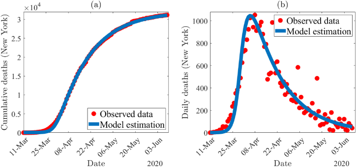
The time series illustration of the least squares fit of the model (2.1) depicted in Fig. 2(a), shows the model output (blue curve) for the cumulative deaths compared to the observed cumulative mortality data (red dots) from the period of March 11th, 2020 to June 9th, 2020 in the state of New York. To show the goodness of the fit, predicted daily mortality from the simulation of the model is compared with the observed daily mortality data (depicted in Fig. 2(b)).

Fig. 2.

(a) Time series illustration of the least squares fit of the model (2.1). It compares the cumulative deaths from model output (blue curve) with the observed cumulative mortality for New York (red dots) from March 11th, 2020 to June 9th, 2020. (b) A comparison of the simulated daily deaths curve (blue) using the fixed and estimated parameter values given in Table 4, Table 5 with the observed data for New York State (in red).

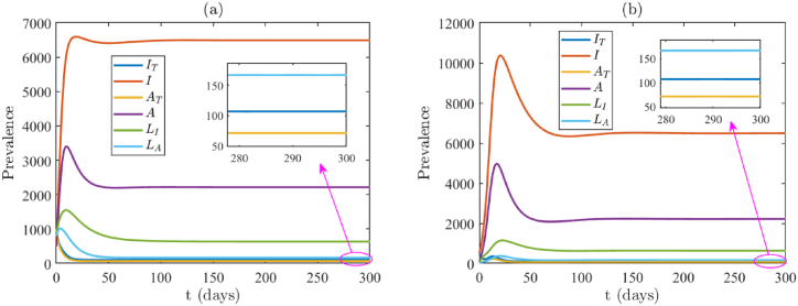
The model (2.1) consists of 17 parameters, of which 6 were obtained from the available literature. We calculated the daily recruitment rate (Λ) as a product of the total population of New York State (19, 453, 561) and the daily natural mortality rate (μ). We assumed the following four parameters for the data fitting of the model: κ = 0.1, σ = 0.1, ϵ_I = 0.1 and ϵ_A = 0.3. Since during the period of our data set, very few tests were done (largely due to lack of testing kits), we assume a testing proportion of κ = σ = 0.1. Since testing was limited, it is reasonable to assume that the vast majority of those who were able to get tested and tested positive were isolation-compliant. Furthermore, it is also sensible to assume that COVID-19 positive tested individuals with symptoms were more likely to comply than those without symptoms. Hence, we chose ϵ_A > ϵ_I, with specific values ϵ_I = 0.1 and ϵ_A = 0.3. The values of these fixed and assumed parameters are tabulated in Table 4. In addition, we estimated the following parameters β_I, β_A, μ_I and ${\mu }_{L_I}$ by using lsqcurvefit in MATLAB 2021a. The package lsqcurvefit uses the least squares regression method, which we use in this project to minimize the total sum of the squared errors (SSE) between the cumulative predicted mortality generated through the model and the observed mortality data. The fitting for the model using the COVID-19 cumulative mortality data for New York is illustrated in Fig. 2(a). The estimated parameter values for the unknown parameters from the data fitting are β_I = 0.4783, β_A = 0.7019, μ_I = 1.0001 × 10⁻⁴ and ${\mu }_{L_I}=5.0546\times 10^{-4}$, which are also tabulated in Table (5). For this set of parameters, the control reproduction number for the model (2.1) is ${\mathcal{R}}_C=7.989$ and the model exhibits a unique endemic equilibrium (given by Theorem 3.2). Due to the complexity of the model, we do not have the result of the stability of the endemic equilibrium. However, in Fig. 3 we show two examples to illustrate its stability and uniqueness using two different sets of initial conditions. The endpoints in both Fig. 3(a) and (b) are approximately.(I_T, I, A_T, A, L_I, L_A) = (107, 6490, 71, 2216, 636, 167), which are the values of the endemic equilibrium computed from the expression in Theorem 3.

Fig. 3.

Endemic equilibria when ${\mathcal{R}}_C=7.989$. In (a) and (b) two different random initial conditions are taken, illustrating that when ${\mathcal{R}}_C>1$, the endemic equilibrium is stable. Initial conditions for (a) and (b) are (S(0), I_T(0), I(0), A_T(0), A(0), L_I(0), L_A(0), R(0)) = (10000, 1000, 500, 1000, 500, 800, 800, 100) and (S(0), I_T(0), I(0), A_T(0), A(0), L_I(0), L_A(0), R(0)) = (20000, 500, 500, 100, 100, 20, 20, 10000), respectively. They have different infection peaks, but approach the same endemic equilibrium.

4.2. Sensitivity analysis

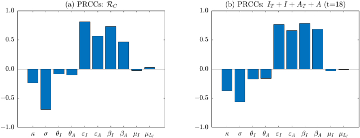
Due to the uncertainty raised from the assumed and estimated parameter values, it is critical to quantify the impact of parameter sensitivities on the dynamics of the model (2.1) (with respect to a particular response function). The analysis performed in Section 3.3 provides the relations between parameters and ${\mathcal{R}}_C$ by elasticity indices. In this section, we use PRCC to quantitatively demonstrate the global uncertainty and sensitivity of parameters on ${\mathcal{R}}_C$ and model dynamics. From the analysis, we know that ${\mathcal{R}}_C$ is the threshold for disease elimination. Thus, we are interested in parameters that have great impact on ${\mathcal{R}}_C$. In addition, we are concerned with the prevalence of the total active infections. Therefore, we choose ${\mathcal{R}}_C$ and I_T + I + A_T + A as our response functions. The inputs are the following assumed and fitted parameters: κ, σ, θ_I, θ_A, ϵ_I, ϵ_A, β_I, β_A, μ_I, ${\mu }_{L_I}$.

We choose parameter values from Table 4, Table 5 as baseline. For the ranges of testing and non-compliance proportions (κ, σ, ϵ_I, ϵ_A), we assume them to be in the interval [0.01, 0.99] so that they remain within the defined domain of (0,1). The ranges for the other parameters are obtained by taking 20% to the left and right of their baseline values. We assume that all parameters obey the uniform distribution. The range of each parameter is separated into 1000 equal sub-intervals. Parameter sets are drawn from this space without replacement, which leads to a 1, 000 × 10 parameter matrix. Then ${\mathcal{R}}_C$ and I_T + I + A_T + A are derived and simulated for each column of this parameter matrix, and PRCCs are then computed. The negative or positive sign of PRCC values represents negative or positive correlation between parameters and the response functions ${\mathcal{R}}_C$ and I_T + I + A_T + A. High PRCC values near −1 or +1 are considered to be substantially linked with the response function (Marino et al., 2008).

Fig. 4(a) shows PRCCs of assumed and fitted parameters on ${\mathcal{R}}_C$. We can see that the magnitude of PRCC values for κ, σ, ϵ_I, ϵ_A, β_I, and β_A are relatively large (see Table 6 for exact values). This indicates that they have more significant influence on ${\mathcal{R}}_C$. We recall that κ, σ, ϵ_I, ϵ_A represent proportions for testing and compliance with isolation, and β_I, β_A are infection rates. Therefore, the above result implies that testing and isolation are effective strategies to mitigate the transmission of COVID-19. Reducing the infection rate by wearing masks or social distancing is also important. Similar results are found in Fig. 4(b), which shows PRCCs of assumed and fitted parameters on the total active infections I_T + I + A_T + A on day 18. The reason we choose day 18 is that we are more interested in the time point when the infection achieves the peak. From Fig. 2(b) we can see that the peak of daily deaths occurs around day 25. The peak for the infection is usually earlier than that for the death. Therefore, here we choose day 18, i.e., one week earlier than the peak of the death. Note that the results derived from both elasticity analysis in Section 3 and sensitivity analysis here agree with each other.

Fig. 4.

Partial rank correlation coefficients (PRCCs) of assumed and fitted parameters on the control reproduction number ${\mathcal{R}}_C$ (as shown in (a)) and the total active infections I_T + I + A_T + A on day 18 (as shown in (b)). The baseline values of the parameters are as given in Table 4, Table 5

Table 6.

Table of PRCC values with assumed and fitted parameters for ${\mathcal{R}}_C$ and I_T + I + A_T + A. The larger PRCC values are indicated with ∗, implying that the corresponding parameters are more significant.

Parameter	PRCC: ${\mathcal{R}}_C$	PRCC:IT + I + AT + A(t = 18)
κ	−0.234∗	−0.371∗
σ	−0.693∗	−0.564∗
θI	−0.085	−0.170
θA	−0.104	−0.163
μI	−0.027	−0.032
${\mu }_{L_I}$	0.028	−0.007
ϵI	0.811∗	0.762∗
ϵA	0.567∗	0.655∗
βI	0.725∗	0.778∗
βA	0.465∗	0.681∗

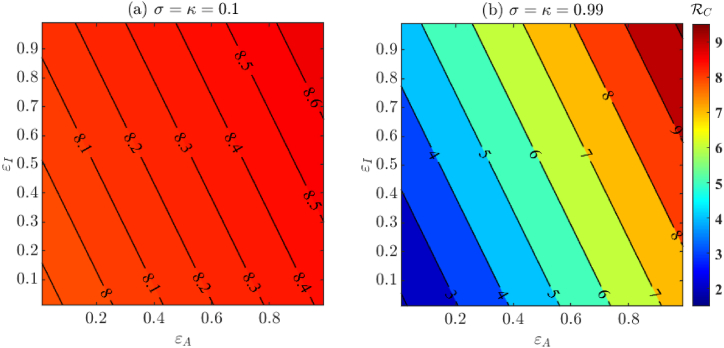
In Fig. 5, we visualize the effect of varying non-compliance on the control reproduction number ${\mathcal{R}}_C$. In Fig. 5(a) we use baseline fixed and fitted parameters from Table 4, Table 5 respectively, whereas in Fig. 5(b) we assume perfect testing (σ = κ = 0.99). From Fig. 5(a) we conclude that under the baseline testing conditions (σ = κ = 0.1), changing isolated compliance behavior is inefficient in controlling ${\mathcal{R}}_C$. In fact, Fig. 5(a) also suggests that if the testing proportion is low, then high isolation compliance on its own may not be a sufficient measure for controlling the spread of the disease. Additionally, from Fig. 5(b) we conclude that reducing ${\mathcal{R}}_C$ below 1 through testing and isolation only is not possible. Additional measures are needed to reduce ${\mathcal{R}}_C$.

Fig. 5.

The effect of varying isolation non-compliance on ${\mathcal{R}}_C$ for imperfect testing σ = κ = 0.1 (shown in (a)) and near perfect testing σ = κ = 0.99 (shown in (b)). Here ϵ_I and ϵ_A denote the non-compliant isolation proportion for symptomatic and asymptomatic infections, respectively. Other parameter values are from Table 4, Table 5

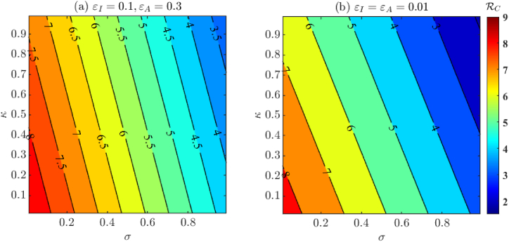
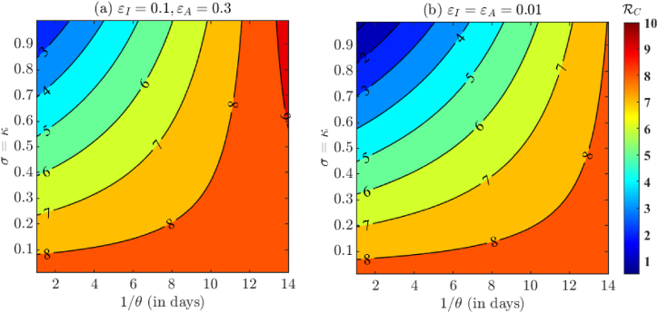
In Fig. 6, we visualize the effect of the proportion of tested COVID-19 individuals on the control reproduction number ${\mathcal{R}}_C$. Specifically, κ is the proportion of asymptomatic individuals who are tested, whereas σ is the proportion of symptomatic individuals who are tested. Fig. 6(a) corresponds to varying σ and κ with other baseline fixed and fitted parameters from Table 4, Table 5 respectively, whereas Fig. 6(b) corresponds to near perfect isolation compliance among individuals having positive test results (ϵ_I = ϵ_A = 0.01). From Fig. 6 we once again conclude that although testing and isolation compliance are important factors in controlling the spread of COVID-19, they are not enough to bring the control reproduction number below unity. Hence, additional control measures are needed.In Fig. 7 we visualize the effect of varying testing turnaround time and testing proportion. We notice that decreasing the turnaround time has a major impact on reduction of ${\mathcal{R}}_C$. In fact, Fig. 7(b) shows that it is even possible for ${\mathcal{R}}_C$ to be below one if a large proportion of individuals are tested with fast testing turnaround and high isolation compliance. It is worth pointing out that the ${\mathcal{R}}_C$ for the duration relevant to our study was 7.989, which may have demanded strict control strategies to obtain ${\mathcal{R}}_C<1$.

Fig. 6.

The effect of varying proportions of tested individuals among symptomatic (κ) and asymptomatic (σ) individuals on ${\mathcal{R}}_C$. Fig. 6(a) has baseline fixed and fitted parameters from Table 4, Table 5 respectively, whereas Fig. 6(b) has near perfect isolation compliance (ϵ_I = ϵ_A = 0.01).

Fig. 7.

The effect of varying testing turnaround time (1/θ) and testing proportions (σ, κ) on ${\mathcal{R}}_C$. The value of θ = θ_I = θ_A is taken to be in [1/14, 1] which corresponds to a testing turnaround time of 1–14 days. Furthermore, for simplicity, we choose σ = κ. Fig. 7(a) has baseline fixed and fitted parameters from Table 4, Table 5 respectively, whereas Fig. 7(b) has near perfect isolation compliance (ϵ_I = ϵ_A = 0.01).

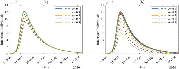
To investigate the impact of COVID-19 testing among infected individuals, we varied testing proportions κ and σ with other parameter values from Table 4, Table 5 Fig. 8(a) and (b) show the daily number of infectious individuals (A_T + A + I_T + I) by varying κ and σ values, respectively. In Fig. 8, solid lines are the results with higher non-compliance proportions (ϵ_A = ϵ_I = 0.7), and the dashed lines are with lower non-compliance proportions (ϵ_A = ϵ_I = 0.01). The number of infected individuals is larger with higher non-compliance proportions (solid lines) than with lower non-compliance proportions (dashed lines), and there is not much effect of testing proportion under the higher non-compliance proportions. Under lower non-compliance, the peak size is reduced by about 20% when the testing proportion among asymptomatic individuals is increased from κ = 0.1 to κ = 0.9 in Fig. 8(a), whereas the size is reduced by about 39% when the testing proportion among symptomatic individuals is increased from σ = 0.1 to σ = 0.9 in Fig. 8(b).

Fig. 8.

The number of infectious individuals (A_T + A + I_T + I) by varying tested proportions κ and σ, respectively. The solid lines correspond to higher non-compliance proportions ϵ_A = ϵ_I = 0.7 and the dashed lines correspond to lower non-compliance proportions ϵ_A = ϵ_I = 0.01.

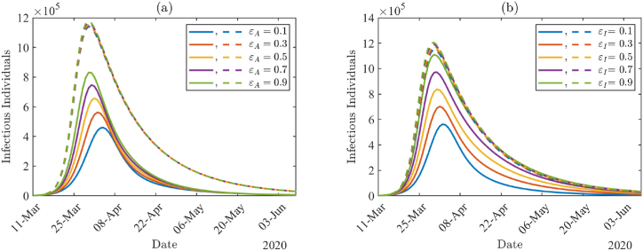
Fig. 9(a) and (b) demonstrate the impact of non-compliance proportions and show the daily number of infectious individuals (A_T + A + I_T + I) by varying ϵ_A and ϵ_I values, respectively. In Fig. 9, solid lines correspond to higher testing proportions (κ = σ = 0.99), and the dashed lines correspond to lower testing proportions (κ = σ = 0.1). The number of infected individuals is larger with lower testing proportions (dashed lines) than with higher testing proportions (solid lines), and there is almost no effect of non-compliance proportions under the lower testing proportions. Under higher testing proportions (solid lines), the peak size of the outbreak is reduced and delayed as each non-compliance proportion decreases in Fig. 9(a) and (b). The peak size is increased by about 81% when the non-compliance proportion among asymptomatic individuals increases from ϵ_A = 0.1 to ϵ_A = 0.9 in Fig. 9(a), whereas the peak size is increased by about 97% when the non-compliance proportion among symptomatic individuals increases from ϵ_I = 0.1 to ϵ_I = 0.9 in Fig. 9(b).

Fig. 9.

The number of infectious individuals (A_T + A + I_T + I) by varying non-compliance proportions ϵ_A and ϵ_I. The solid lines correspond to higher testing proportions values κ = σ = 0.99, and the dashed lines correspond to lower testing proportions κ = σ = 0.1.

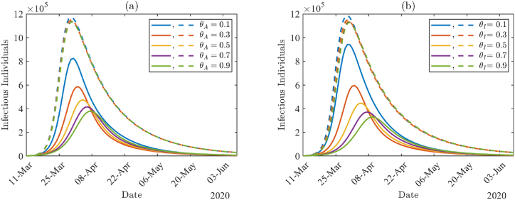
In Fig. 10, we study the impact of test waiting time on the prevalence of infectious individuals (A_T + A + I_T + I) by varying θ_A and θ_I since 1/θ_A and 1/θ_A represent the waiting time. Here, solid lines correspond to higher testing proportions (κ = σ = 0.99), and the dashed lines correspond to lower testing proportions (κ = σ = 0.1). We can see that in both cases, there are more infectious individuals with lower testing proportions (dashed lines) compared to higher testing proportions (solid lines). In addition, there is almost no effect of waiting time on the prevalence under the lower testing proportions. In contrast, under higher testing proportions (solid lines), the peak size of the outbreak can be reduced and delayed as waiting time decreases. More specifically, the peak size is decreased by about 54% (see Fig. 10(a)) and 65% (see Fig. 10(b)) when the waiting rate among asymptomatic individuals (θ_A) or symptomatic individuals (θ_I) increases from 0.1 to 0.9.

Fig. 10.

The number of infectious individuals (A_T + A + I_T + I) by varying test waiting rates θ_A and θ_I. The solid lines correspond to higher testing proportions values κ = σ = 0.99, and the dashed lines correspond to lower testing proportions κ = σ = 0.1.

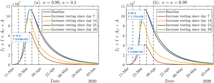
From above, we know that high testing proportion combined with high compliance to isolation can significantly reduce the prevalence of the total active infections. In addition, prompt response to the pandemic is also important. Therefore, in Fig. 11 we investigate the impact of starting dates of increasing testing capacity by assuming near perfect testing and near perfect compliance to isolation. In the early stage of the pandemic, there was a lack of testing resources in the US and worldwide. Back then, only symptomatic infected individuals were tested. We are also interested in the effect that mass testing would have had on the course of the pandemic. Therefore, two scenarios were considered, i.e., increasing testing by near perfect testing only for symptomatic individuals (σ = 0.99, κ = 0.1) or by near perfect mass testing (σ = κ = 0.99). Both Fig. 11(a) and (b) show that if we increase the testing capacity before the infection peak, then the prevalence of the total active infection can be significantly reduced. For example, if we adopt near perfect mass testing, then more than 60% of infections could be reduced (see Fig. 11(b)). However, if the increase in testing capacity is implemented after the infection peak, there is only minor influence. In addition, if we focus on a specific case, namely, increase in testing since day 7, and compare Fig. 11(a) and (b), it can be seen that mass testing can reduce many more infections than only testing symptomatic individuals. However, if we compare the other 3 cases, the difference between the two pictures is not much. This again emphasizes the importance of early implementation of increased testing capacity.

Fig. 11.

(a): The total active infections given different starting dates of improving testing. Here we assume the baseline to be σ = κ = 0.1. Improving testing in (a) and (b) refer to only testing symptomatic individuals (σ = 0.99, κ = 0.1) and mass testing strategy (σ = κ = 0.99), respectively. In both panels ϵ_I = ϵ_A = 0.01, and all the other parameter values are from Tables (4) and (5).

5. Discussion and conclusion

In Section 2 of this paper, we developed a deterministic model to investigate the impact of testing and isolation compliance on the spread of COVID-19 transmission. More specifically, we aimed to compare the impact of testing and isolation compliance of symptomatic individuals with that of asymptomatic individuals. So, we considered both symptomatic and asymptomatic transmission and split each class into two subclasses, i.e., tested classes (I_T and A_T) and non-tested or tested but not isolated classes (I and A). This is a novel feature of our model, and facilitates discussion of the impact of testing and isolation.

In Section 3.1, we obtained the control reproduction number ${\mathcal{R}}_C$ (given by Equation (3.1)) and interpreted its biological meaning. Rigorous analyses of the local and global stability of the disease-free equilibrium are given in Section 3.2. We also derived the explicit form of the endemic equilibrium. However, due to the complexity of the endemic equilibrium, its stability was only numerically investigated. We calibrated model (2.1) using cumulative mortality data of the early stage of the pandemic in New York State. The fixed and fitted parameter values are listed in Table 4, Table 5, respectively. Based on these parameter values, we computed the control reproduction number ${\mathcal{R}}_C=7.989$. This value is larger than that given in (Ives & Bozzuto, 2020), where 6.4 is the estimate for the basic reproduction number ${\mathcal{R}}_0$ at the beginning of the outbreak in New York State. Another study estimated ${\mathcal{R}}_0$ in New York State to be in the range 3.2–8.1 (Subramanian et al., 2021). Using data from New York and other countries, Kochańczyk et al. derived a larger range, namely 4.7 − 11.4 (Kochańczyk et al., 2020). Our estimation is within these ranges. Possible reasons for the large ranges may include usage of different data sources (we used John Hopkins, but there are numerous other data sets, such as that of the New York Times), the study being conducted during different periods, models being fit to different data sets (we fitted mortality data, but most studies fitted daily case data that is far less reliable, especially in the early phase of the pandemic with limited testing capabilities), and of course difference in the models themselves.

To reduce the spread of COVID-19, it is important to lower the ${\mathcal{R}}_C$ value. To achieve this, it is necessary to understand the impact that various parameters have on ${\mathcal{R}}_C$. In Section 3.3, we performed an elasticity analysis to determine positive or negative changes that key parameters have on ${\mathcal{R}}_C$. Furthermore, using the values of fixed and fitted parameters reported in Table 4, Table 5, we calculated sensitivity indices of various key parameters on ${\mathcal{R}}_C$ and listed these in Table 3. This is a local sensitivity approach. We also considered a global approach using the PRCC method in Section 4.2. Both methods suggest that testing and compliance with isolation are important for disease control. Additionally, from Fig. 5, Fig. 6, Fig. 7, Fig. 8, Fig. 9, Fig. 10, we concluded that a high testing volume combined with a high proportion of compliance to isolation as well as a short waiting time for test results are needed to slow down the transmission, namely, the peak of infection is lowered and delayed. In Fig. 11, we discussed the importance of the early implementation of increased testing. In addition, we showed that mass testing can reduce more infections compared to testing only symptomatic individuals.

The above results are consistent with those from several other studies. For example, Kucharski at al (Kucharski et al., 2020). showed that in order to lower the effective reproduction number to be less than 1, a high proportion of cases need to self-isolate and a high proportion of their contacts need to be successfully traced. Howerton et al. (Howerton et al., 2021) emphasized the importance of a high proportion of testing. They also pointed out that only mass testing followed by short test delays as well as isolation can mitigate the reliance on distancing. Here mass testing represents testing in the general population regardless of the presentation of symptoms. It was used in some regions and was widely discussed during the COVID-19 pandemic. Aronna et al. (Aronna et al., 2021) demonstrated that testing among asymptomatic infections is fundamental to control the epidemic. The stricter the testing and isolation and the sooner they are implemented, the more effective they are in flattening the curve of infections. This silent transmission of COVID-19 was also discussed in (Moghadas et al., 2020). They found that except for symptom-based isolation, identifying asymptomatic and presymptomatic cases are key factors to minimize the risk of resurgence. Wells et al. (Wells et al., 2021) also pointed out that even perfect isolation of all symptomatic individuals would not be sufficient to curb the chain of disease transmission. The importance of early implementation of control strategies was also studied in several papers. For example, He et al. (He et al., 2021) showed that timely screening and detection would be needed to avoid future waves. Knock et al. (Knock et al., 2021) concluded that if the lockdown could have been implemented one week earlier, then approximately half of the mortality in England would have been avoided.

We acknowledge that the model presented in this paper does not capture all the features of COVID-19. Since we mainly focus on the impact of testing and compliance of isolation on the transmission of COVID-19, we do not include an exposed (but not infectious) class, which is also not considered in some other papers modeling COVID-19 (Calleri et al., 2021; Massard et al., 2022; Serhani & Labbardi, 2021). Another limitation is that the actual size of the epidemic is unknown, which means that we do not know the exact proportion of asymptomatic and symptomatic people who were tested, especially at the early phase of the pandemic. The impacts of testing and isolation may vary as the pandemic develops. However, this variation was not considered in this paper since we mainly focus on the early stage of the pandemic, and aim to compare the impact of testing and isolation compliance of symptomatic individuals with that of asymptomatic individuals. This variation is an interesting topic for future research.

In summary, we built a deterministic model to investigate the impact of testing and isolation compliance on the early stage of transmission of COVID-19. Even though the data are from New York State, the control strategies considered here are only testing and isolation, whereas physical distancing and masking may have also been implemented. However, the results derived here could be adapted to other control strategies, for other diseases similar to COVID-19, and in other regions.

Handling Editor: Dr Yijun Lou

Appendix A. Control Reproduction Number

We consider the infected classes (I_T, I, A_T, A, L_I, L_A). Taking the Jacobian matrix at the DFE E⁰ and writing it as the matrix of new infections F minus the matrix of transfers V gives

$$F=\left(\begin{array}{cccccc}\sigma \delta {\beta }_I& \sigma \delta {\beta }_I& \sigma \delta {\beta }_A& \sigma \delta {\beta }_A& 0& 0\\ (1-\sigma )\delta {\beta }_I& (1-\sigma )\delta {\beta }_I& (1-\sigma )\delta {\beta }_A& (1-\sigma )\delta {\beta }_A& 0& 0\\ \kappa (1-\delta ){\beta }_I& \kappa (1-\delta ){\beta }_I& \kappa (1-\delta ){\beta }_A& \kappa (1-\delta ){\beta }_A& 0& 0\\ (1-\kappa )(1-\delta ){\beta }_I& (1-\kappa )(1-\delta ){\beta }_I& (1-\kappa )(1-\delta ){\beta }_A& (1-\kappa )(1-\delta ){\beta }_A& 0& 0\\ 0& 0& 0& 0& 0& 0\\ 0& 0& 0& 0& 0& 0\end{array}\right),$$

$$V=\left(\begin{array}{cccccc}\mu +{\mu }_I+{\theta }_I& 0& 0& 0& 0& 0\\ -{ϵ}_I{\theta }_I& \mu +{\mu }_I+{\gamma }_I& 0& 0& 0& 0\\ 0& 0& \mu +{\theta }_A& 0& 0& 0\\ 0& 0& -{ϵ}_A{\theta }_A& \mu +{\gamma }_A& 0& 0\\ -(1-{ϵ}_I){\theta }_I& 0& 0& 0& \mu +{\mu }_{L_I}+{\gamma }_{L_I}& 0\\ 0& 0& -(1-{ϵ}_A){\theta }_A& 0& 0& \mu +{\gamma }_{L_A}\end{array}\right).$$

Then the next-generation matrix is written as $F{V}^{-1}={(a_{ij})}_{6\times 6}$, where the non-zero entries in FV⁻¹ are

$$a_{11}=\sigma \delta {\mathcal{R}}_{C,I_T},a_{12}=\sigma \delta {\mathcal{R}}_{C,I},a_{13}=\sigma \delta {\mathcal{R}}_{C,A_T},a_{14}=\sigma \delta {\mathcal{R}}_{C,A}{a}_{2j}=\frac{1-\sigma }{\sigma }{a}_{1j},a_{3j}=\frac{\kappa (1-\delta )}{\sigma \delta }{a}_{1j},a_{4j}=\frac{(1-\kappa )(1-\delta )}{\sigma \delta }{a}_{1j},j=1,\dots ,4,$$

with $R_{C,I_T}$, R_C,I, $R_{C,A_T}$, R_C,A as stated in (3.2).

The matrix FV⁻¹ has rank 1. Thus, it has at most one non-zero eigenvalue $\overline{\lambda }$. Since trace(FV⁻¹) is the sum of all eigenvalues of FV⁻¹, $\overline{\lambda }=trace(F{V}^{-1})$. Therefore, the control reproduction number ${\mathcal{R}}_C=\rho (F{V}^{-1})=trace(F{V}^{-1})=a_{11}+a_{22}+a_{33}+a_{44}$, where ρ(FV⁻¹) is the spectral radius of matrix FV⁻¹.

Appendix B. Proof of Theorem 2

Using the method introduced in Theorem 2.1 in (Shuai & van den Driessche, 2013), we define the following Lyapunov function,

$$L={\mathcal{R}}_{C,I_T}{I}_T+{\mathcal{R}}_{C,I}I+{\mathcal{R}}_{C,A_T}{A}_T+{\mathcal{R}}_{C,A}A.$$

It is clear that L is radially unbounded and positive definite in the entire space Ω. The derivative of L along the trajectories of system (2.1) yields

$$\dot{L}={\mathcal{R}}_{C,I_T}{\dot{I}}_T+{\mathcal{R}}_{C,I}\dot{I}+{\mathcal{R}}_{C,A_T}{\dot{A}}_T+{\mathcal{R}}_{C,A}\dot{A}={\mathcal{R}}_{C,I_T}[\sigma \delta ({\lambda }_I+{\lambda }_A)S-(\mu +{\mu }_I+{\theta }_I)I_T]+{\mathcal{R}}_{C,I}[(1-\sigma )\delta ({\lambda }_I+{\lambda }_A)S+{ϵ}_I{\theta }_I{I}_T-(\mu +{\mu }_I+{\gamma }_I)I]+{\mathcal{R}}_{C,A_T}[\kappa (1-\delta )({\lambda }_I+{\lambda }_A)S-(\mu +{\theta }_A)A_T]+{\mathcal{R}}_{C,A}[(1-\kappa )(1-\delta )({\lambda }_I+{\lambda }_A)S+{ϵ}_A{\theta }_A{A}_T-(\mu +{\gamma }_A)A]={\mathcal{R}}_C\left[\frac{{\beta }_I(I_T+I)S}{S+I_T+I+A_T+A+R}+\frac{{\beta }_A(A_T+A)S}{S+I_T+I+A_T+A+R}\right]+[-{\mathcal{R}}_{C,I_T}(\mu +{\mu }_I+{\theta }_I)+{\mathcal{R}}_{C,I}{ϵ}_I{\theta }_I]I_T-{\mathcal{R}}_{C,I}(\mu +{\mu }_I+{\gamma }_I)I+[-{\mathcal{R}}_{C,A_T}(\mu +{\theta }_A)+{\mathcal{R}}_{C,A}{ϵ}_A{\theta }_A]A_T-{\mathcal{R}}_{C,A}(\mu +{\gamma }_A)A.$$

Using the expressions in (3.2), we have

$$-{\mathcal{R}}_{C,I_T}(\mu +{\mu }_I+{\theta }_I)+{\mathcal{R}}_{C,I}{ϵ}_I{\theta }_I=-{\beta }_I,{\mathcal{R}}_{C,I}(\mu +{\mu }_I+{\gamma }_I)={\beta }_I,-{\mathcal{R}}_{C,A_T}(\mu +{\theta }_A)+{\mathcal{R}}_{C,A}{ϵ}_A{\theta }_A=-{\beta }_A,{\mathcal{R}}_{C,A}(\mu +{\gamma }_A)={\beta }_A.$$

Since

$$\frac{S}{S+I_T+I+A_T+A+R}\le 1,$$

it follows that

$$\dot{L}\le ({\mathcal{R}}_C-1)({\beta }_I{I}_T+{\beta }_{I}I+{\beta }_A{A}_T+{\beta }_{A}A).$$

Thus if ${\mathcal{R}}_C<1$, $\dot{L}\le 0$, with equality holding at the DFE. By LaSalle's Theorem (LaSalle, 1960), the DFE E⁰ is globally asymptotically stable when ${\mathcal{R}}_C<1$.

Appendix C. Proof of Theorem 3

To obtain the endemic equilibrium, we set the right-hand side of system (2.1) to zero, resulting in the following system of equations.

$$\mathrm{\Lambda }-\mu S-({\lambda }_I+{\lambda }_A)S=0$$ (C.1)

$$\sigma \delta ({\lambda }_I+{\lambda }_A)S-(\mu +{\mu }_I+{\theta }_I)I_T=0$$ (C.2)

$$(1-\sigma )\delta ({\lambda }_I+{\lambda }_A)S+{ϵ}_I{\theta }_I{I}_T-(\mu +{\mu }_I+{\gamma }_I)I=0$$ (C.3)

$$\kappa (1-\delta )({\lambda }_I+{\lambda }_A)S-(\mu +{\theta }_A)A_T=0$$ (C.4)

$$(1-\kappa )(1-\delta )({\lambda }_I+{\lambda }_A)S+{ϵ}_A{\theta }_A{A}_T-(\mu +{\gamma }_A)A=0$$ (C.5)

$$(1-{ϵ}_I){\theta }_I{I}_T-(\mu +{\mu }_{L_I}+{\gamma }_{L_I})L_I=0$$ (C.6)

$$(1-{ϵ}_A){\theta }_A{A}_T-(\mu +{\gamma }_{L_A})L_A=0$$ (C.7)

$${\gamma }_{I}I+{\gamma }_{A}A+{\gamma }_{L_I}{L}_I+{\gamma }_{L_A}{L}_A-\mu R=0$$ (C.8)

Equation (C.2) gives

$$({\lambda }_I+{\lambda }_A)S=\frac{\mu +{\mu }_I+{\theta }_I}{\sigma \delta }{I}_T.$$

Substituting the preceding equation into (C.3)-(C.8) gives

$$I=a_1{I}_T,A_T=a_2{I}_T,A=a_3{I}_T,L_I=a_4{I}_T,L_A=a_5{I}_T,R=a_6{I}_T,$$ (C.9)

where a_i (i = 1, …, 6) are stated in (3.3).

Substituting (C.9) into (C.2) gives

$$\sigma \delta \frac{[{\beta }_I(1+a_1)+{\beta }_A(a_2+a_3)]I_{T}S}{S+I_T+I+A_T+A+R}=(\mu +{\mu }_I+{\theta }_I)I_T.$$ (C.10)

The preceding equation holds in the following two cases. (1) If I_T = 0, from (C.9) and (C.1), we have I = A_T = A = L_I = L_A = R = 0 and $S=\frac{\mathrm{\Lambda }}{\mu }$. This is the DFE.

(2) If I_T ≠ 0, dividing by I_T on both sides of (C.10) and rearrange the equation gives:

$$\sigma \delta \frac{{\beta }_I(1+a_1)+{\beta }_A(a_2+a_3)}{\mu +{\mu }_I+{\theta }_I}=\frac{S+I_T+I+A_T+A+R}{S}.$$ (C.11)

We notice that

$$\begin{array}{cc}\sigma \delta \frac{{\beta }_I(1+a_1)}{\mu +{\mu }_I+{\theta }_I}& =\frac{\sigma \delta {\beta }_I}{\mu +{\mu }_I+{\theta }_I}+\frac{\sigma \delta {\beta }_I{ϵ}_I{\theta }_I}{(\mu +{\mu }_I+{\theta }_I)(\mu +{\mu }_I+{\gamma }_I)}+\frac{(1-\sigma )\delta {\beta }_I}{\mu +{\mu }_I+{\gamma }_I}\\ & =\sigma \delta {\mathcal{R}}_{C,I_T}+(1-\sigma )\delta {\mathcal{R}}_{C,I}\end{array}$$

and

$$\begin{array}{cc}\sigma \delta \frac{{\beta }_A(a_2+a_3)}{\mu +{\mu }_I+{\theta }_I}& =\frac{\kappa (1-\delta ){\beta }_A}{\mu +{\theta }_A}+\frac{\kappa (1-\sigma ){ϵ}_A{\theta }_A{\beta }_A}{(\mu +{\theta }_A)(\mu +{\gamma }_A)}+\frac{(1-\kappa )(1-\sigma ){\beta }_A}{\mu +{\gamma }_A}\\ & =\kappa (1-\delta ){\mathcal{R}}_{C,A_T}+(1-\kappa )(1-\delta ){\mathcal{R}}_{C,A}.\end{array}$$

Therefore, (C.11) can be rewritten as follows:

$${\mathcal{R}}_C=\frac{S+I_T+I+A_T+A+R}{S}.$$ (C.12)

This is valid only when ${\mathcal{R}}_C>1$. Rearranging the above equation gives

$$I_T=\frac{{\mathcal{R}}_C-1}{1+a_1+a_2+a_3+a_6}S.$$ (C.13)

Taking the sum of equations (C.1)-(C.8) and solving for N yields,

$$N=\frac{1}{\mu }\left[\mathrm{\Lambda }-({\mu }_I+a_1{\mu }_I+a_4{\mu }_{L_I})I_T\right]=S+\left(1+\sum _{j=1}^6{a}_j\right)I_T.$$

It follows that

$$S=\frac{\mathrm{\Lambda }}{\mu +\left[{\mu }_I+a_1{\mu }_I+a_4{\mu }_{L_I}+\mu \left(1+{\sum }_{j=1}^6{a}_j\right)\right]\frac{{\mathcal{R}}_C-1}{1+a_1+a_2+a_3+a_6}}.$$

Since all parameter values are positive and all proportions δ, σ, κ, ϵ_I, ϵ_A ∈ (0, 1), a_j > 0 for j = 1, 2, …, 6. Then positive S exists if and only if ${\mathcal{R}}_C>1$. From (C.13) and (C.9) we know that the values of all the components of (S, I_T, I, A_T, A, L_I, L_A, R) are positive. Therefore, there exists a unique endemic equilibrium as given above if and only if ${\mathcal{R}}_C>1$.

References

- Almagor J., Picascia S. Exploring the effectiveness of a COVID-19 contact tracing app using an agent-based model. Scientific Reports. 2020;10(1 10):1–11. doi: 10.1038/s41598-020-79000-y. 12 2020. [DOI] [PMC free article] [PubMed] [Google Scholar]
- Álvarez L., Rojas-Galeano S. medRxiv; 2020. Simulation of non-pharmaceutical interventions on COVID-19 with an agent-based model of zonal restraint. 6 2020. 06.13.20130542. [Google Scholar]
- Aronna M.S., Guglielmi R., Moschen L.M. A model for COVID-19 with isolation, quarantine and testing as control measures. Epidemics. 2021;34 doi: 10.1016/j.epidem.2021.100437. 3. [DOI] [PMC free article] [PubMed] [Google Scholar]
- Bartha F.A., Karsai J., Tekeli T., Röst G. Analysis of infectious disease problems (Covid-19) and their global impact. Springer; 2021. Symptom-based testing in a compartmental model of covid-19; pp. 357–376. [Google Scholar]
- Bhaduri R., Kundu R., Purkayastha S., Kleinsasser M., Beesley L.J., Mukherjee B., Datta J., 6 Extending the susceptible-exposed-infected-removed (SEIR) model to handle the false negative rate and symptom-based administration of COVID-19 diagnostic tests: SEIR-fansy. Statistics in Medicine. 2022;41:2317–2337. doi: 10.1002/sim.9357. [DOI] [PMC free article] [PubMed] [Google Scholar]
- Bodas M., Peleg K., 6 Self-isolation compliance in the covid-19 era influenced by compensation: Findings from a recent survey in Israel. Health Affairs. 2020;39:936–941. doi: 10.1377/hlthaff.2020.00382. [DOI] [PubMed] [Google Scholar]
- Brozak S.J., Pant B., Safdar S., Gumel A.B. Dynamics of COVID-19 pandemic in India and Pakistan: A metapopulation modelling approach. Infectious Disease Modelling. 2021;6:1173–1201. doi: 10.1016/j.idm.2021.10.001. [DOI] [PMC free article] [PubMed] [Google Scholar]
- Calleri F., Nastasi G., Romano V. Continuous-time stochastic processes for the spread of COVID-19 disease simulated via a Monte Carlo approach and comparison with deterministic models. Journal of Mathematical Biology. 2021;83(4):1–26. doi: 10.1007/s00285-021-01657-4. [DOI] [PMC free article] [PubMed] [Google Scholar]
- CDC Centers for disease control and prevention, CDC Museum COVID-19 timeline. https://www.cdc.gov/museum/timeline/covid19.html
- Center for Systems Science and Engineering at Johns Hopkins University . 2020. CSSEGISandData/COVID-19. [Google Scholar]
- Cleveland Clinic, (Accessed March 1, 2022). Coronavirus, COVID-19.
- Cohen J. Science Magazine; 2020. The United States badly bungled coronavirus testing—but things may soon improve; science; aaas. [Google Scholar]
- Dong E., Du H., Gardner L. An interactive web-based dashboard to track Covid-19 in real time. The Lancet Infectious Diseases. 2020;20(5):533–534. doi: 10.1016/S1473-3099(20)30120-1. [DOI] [PMC free article] [PubMed] [Google Scholar]
- van den Driessche P. Reproduction numbers of infectious disease models. Infectious Disease Modelling. 2017;2(3):288–303. doi: 10.1016/j.idm.2017.06.002. [DOI] [PMC free article] [PubMed] [Google Scholar]
- van den Driessche P., Watmough J. Reproduction numbers and sub-threshold endemic equilibria for compartmental models of disease transmission. Mathematical Biosciences. 2002;180(1–2):29–48. doi: 10.1016/s0025-5564(02)00108-6. [DOI] [PubMed] [Google Scholar]
- Eikenberry S.E., Mancuso M., Iboi E., Phan T., Eikenberry K., Kuang Y., Kostelich E., Gumel A.B. To mask or not to mask: Modeling the potential for face mask use by the general public to curtail the COVID-19 pandemic. Infectious Disease Modelling. 2020;5:293–308. doi: 10.1016/j.idm.2020.04.001. [DOI] [PMC free article] [PubMed] [Google Scholar]
- Gao S., Martcheva M., Miao H., Rong L. A dynamic model to assess human papillomavirus vaccination strategies in a heterosexual population combined with men who have sex with men. Bulletin of Mathematical Biology. 2021;83(1):1–36. doi: 10.1007/s11538-020-00830-y. [DOI] [PubMed] [Google Scholar]
- Gumel A.B., Iboi E.A., Ngonghala C.N., Ngwa G.A. Toward achieving a vaccine-derived herd immunity threshold for COVID-19 in the US. Frontiers in Public Health. 2021;9 doi: 10.3389/fpubh.2021.709369. [DOI] [PMC free article] [PubMed] [Google Scholar]
- Hahn S.M., Shuren J.E. 2020. Coronavirus (COVID-19) update: FDA authorizes first antigen test to help in the rapid detection of the virus that causes COVID-19 in patients. 05-09. [Google Scholar]
- Health, N., Hospitals, 2022(Accessed June 30, 2022). Test and Trace Corps-Testing.
- He X., Lau E.H., Wu P., Deng X., Wang J., Hao X., Lau Y.C., Wong J.Y., Guan Y., Tan X., et al. Temporal dynamics in viral shedding and transmissibility of COVID-19. Nature Medicine. 2020;26(5):672–675. doi: 10.1038/s41591-020-0869-5. [DOI] [PubMed] [Google Scholar]
- He S., Yang J., He M., Yan D., Tang S., Rong L. The risk of future waves of COVID-19: Modeling and data analysis. Mathematical Biosciences and Engineering. 2021;18(5) doi: 10.3934/mbe.2021274. [DOI] [PubMed] [Google Scholar]
- Hoogenboom W.S., Pham A., Anand H., Fleysher R., Buczek A., Soby S., Mirhaji P., Yee J., Duong T.Q. Clinical characteristics of the first and second COVID-19 waves in the Bronx, New York: A retrospective cohort study. The Lancet Regional Health-Americas. 2021;3 doi: 10.1016/j.lana.2021.100041. [DOI] [PMC free article] [PubMed] [Google Scholar]
- Howerton E., Ferrari M.J., Bjørnstad O.N., Bogich T.L., Borchering R.K., Jewell C.P., Nichols J.D., Probert W.J., Runge M.C., Tildesley M.J., Viboud C., Shea K., 10 Synergistic interventions to control COVID-19: Mass testing and isolation mitigates reliance on distancing. PLoS Computational Biology. 2021;17 doi: 10.1371/journal.pcbi.1009518. [DOI] [PMC free article] [PubMed] [Google Scholar]
- Ives A.R., Bozzuto C. MedRxiv; 2020. State-by-State estimates of R0 at the start of COVID-19 outbreaks in the USA. [Google Scholar]
- Jackson J.K. Congressional Research Service; 2021. Global economic effects of COVID-19. [Google Scholar]
- Johansson M.A., Quandelacy T.M., Kada S., Prasad P.V., Steele M., Brooks J.T., Slayton R.B., Biggerstaff M., Butler J.C., 1 SARS-CoV-2 transmission from people without COVID-19 symptoms. JAMA Network Open. 2021;4 doi: 10.1001/jamanetworkopen.2020.35057. e2035057–e2035057. [DOI] [PMC free article] [PubMed] [Google Scholar]
- Kim Y.J., Koo P.-H. Effectiveness of testing and contact-tracing to counter COVID-19 pandemic: Designed experiments of agent-based simulation. Healthcare. 2021;9(6):625. doi: 10.3390/healthcare9060625. [DOI] [PMC free article] [PubMed] [Google Scholar]
- Knock E.S., Whittles L.K., Lees J.A., Perez-Guzman P.N., Verity R., FitzJohn R.G., Gaythorpe K.A., Imai N., Hinsley W., Okell L.C., et al. Key epidemiological drivers and impact of interventions in the 2020 SARS-CoV-2 epidemic in England. Science Translational Medicine. 2021;13(602) doi: 10.1126/scitranslmed.abg4262. [DOI] [PMC free article] [PubMed] [Google Scholar]
- Kochańczyk M., Grabowski F., Lipniacki T. Super-spreading events initiated the exponential growth phase of COVID-19 with higher than initially estimated. Royal Society Open Science. 2020;7(9) doi: 10.1098/rsos.200786. [DOI] [PMC free article] [PubMed] [Google Scholar]
- Kucharski A.J., Klepac P., Conlan A., Kissler S.M., Simons D. Effectiveness of isolation, testing, contact tracing, and physical distancing on reducing transmission of SARS-CoV-2 in different settings: A mathematical modelling study. The Lancet Infectious Diseases. 2020;20:1151–1160. doi: 10.1016/S1473-3099(20)30457-6. [DOI] [PMC free article] [PubMed] [Google Scholar]
- LaSalle J. Some extensions of Liapunov's second method. IEEE Transactions on Circuit Theory. 1960;7(4):520–527. [Google Scholar]
- Leontitsis A., Senok A., Alsheikh-Ali A., Nasser Y.A., Loney T., Alshamsi A. SEAHIR: A specialized compartmental model for COVID-19. International Journal of Environmental Research and Public Health. 2021;18 doi: 10.3390/ijerph18052667. 3 2021. 2667 18, 2667. [DOI] [PMC free article] [PubMed] [Google Scholar]
- López Seguí F., Navarrete Duran J.M., Tuldrà A., Sarquella M., Revollo B., Llibre J.M., Ara del Rey J., Estrada Cuxart O., Paredes Deirós R., Hernández Guillamet G., et al. Impact of mass workplace COVID-19 rapid testing on health and healthcare resource savings. International Journal of Environmental Research and Public Health. 2021;18(13):7129. doi: 10.3390/ijerph18137129. [DOI] [PMC free article] [PubMed] [Google Scholar]
- Mancuso M., Eikenberry S.E., Gumel A.B. Will vaccine-derived protective immunity curtail COVID-19 variants in the US? Infectious Disease Modelling. 2021;6:1110–1134. doi: 10.1016/j.idm.2021.08.008. [DOI] [PMC free article] [PubMed] [Google Scholar]
- Marino S., Hogue I.B., Ray C.J., Kirschner D.E. A methodology for performing global uncertainty and sensitivity analysis in systems biology. Journal of Theoretical Biology. 2008;254(1):178–196. doi: 10.1016/j.jtbi.2008.04.011. [DOI] [PMC free article] [PubMed] [Google Scholar]
- Massard M., Eftimie R., Perasso A., Saussereau B. A multi-strain epidemic model for COVID-19 with infected and asymptomatic cases: Application to French data. Journal of Theoretical Biology. 2022;545 doi: 10.1016/j.jtbi.2022.111117. [DOI] [PMC free article] [PubMed] [Google Scholar]
- Moghadas S.M., Fitzpatrick M.C., Sah P., Pandey A., Shoukat A., Singer B.H., Galvani A.P. The implications of silent transmission for the control of COVID-19 outbreaks. Proceedings of the National Academy of Sciences. 2020;117(30):17513–17515. doi: 10.1073/pnas.2008373117. [DOI] [PMC free article] [PubMed] [Google Scholar]
- Oran D.P., Topol E.J. Prevalence of asymptomatic SARS-CoV-2 infection: A narrative review. Annals of Internal Medicine. 2020;173(5):362–367. doi: 10.7326/M20-3012. [DOI] [PMC free article] [PubMed] [Google Scholar]
- Padmanabhan R., Abed H.S., Meskin N., Khattab T., Shraim M., Al-Hitmi M.A., 9 A review of mathematical model-based scenario analysis and interventions for COVID-19. Computer Methods and Programs in Biomedicine. 2021;209 doi: 10.1016/j.cmpb.2021.106301. [DOI] [PMC free article] [PubMed] [Google Scholar]
- Patel J., Fernandes G., Sridhar D. How can we improve self-isolation and quarantine for COVID-19? BMJ. 2021;372 doi: 10.1136/bmj.n625. 3. [DOI] [PubMed] [Google Scholar]
- Patel A., Jernigan D.B., Abdirizak F., Abedi G., Aggarwal S., Albina D., Allen E., Andersen L., Anderson J., Anderson M., et al. Initial public health response and interim clinical guidance for the 2019 novel coronavirus outbreak—United States, December 31, 2019–February 4, 2020. Morbidity and Mortality Weekly Report. 2020;69(5):140. doi: 10.15585/mmwr.mm6905e1. [DOI] [PMC free article] [PubMed] [Google Scholar]
- Seibold M.A., Moore C.M., Everman J.L., Williams B.J., Nolin J.D., Fairbanks-Mahnke A., HEROS study team Risk factors for SARS-CoV-2 infection and transmission in households with children with asthma and allergy: A prospective surveillance study. Journal of Allergy and Clinical Immunology. 2022;150(2):302–311. doi: 10.1016/j.jaci.2022.05.014. [DOI] [PMC free article] [PubMed] [Google Scholar]
- Serhani M., Labbardi H. Mathematical modeling of COVID-19 spreading with asymptomatic infected and interacting peoples. Journal of Applied Mathematics and Computing. 2021;66(1):1–20. doi: 10.1007/s12190-020-01421-9. [DOI] [PMC free article] [PubMed] [Google Scholar]
- Shen M., Xiao Y., Zhuang G., Li Y., Zhang L., 5 Mass testing—an underexplored strategy for COVID-19 control. Innovation. 2021;2 doi: 10.1016/j.xinn.2021.100114. [DOI] [PMC free article] [PubMed] [Google Scholar]
- Shuai Z., van den Driessche P. Global stability of infectious disease models using Lyapunov functions. SIAM Journal on Applied Mathematics. 2013;73(4):1513–1532. [Google Scholar]
- Sturniolo S., Waites W., Colbourn T., Manheim D., Panovska-Griffiths J. Testing, tracing and isolation in compartmental models. PLoS Computational Biology. 2021;17 doi: 10.1371/journal.pcbi.1008633. 3. [DOI] [PMC free article] [PubMed] [Google Scholar]
- Subramanian R., He Q., Pascual M. Quantifying asymptomatic infection and transmission of COVID-19 in New York City using observed cases, serology, and testing capacity. Proceedings of the National Academy of Sciences. 2021;118(9) doi: 10.1073/pnas.2019716118. [DOI] [PMC free article] [PubMed] [Google Scholar]
- Tang B., Bragazzi N.L., Li Q., Tang S., Xiao Y., Wu J. An updated estimation of the risk of transmission of the novel coronavirus (2019-ncov) Infectious Disease Modelling. 2020;5:248–255. doi: 10.1016/j.idm.2020.02.001. [DOI] [PMC free article] [PubMed] [Google Scholar]
- Tseng C.W., Roh Y., DeJong C., Kanagusuku L.N., Soin K.S., 11 Patients' compliance with quarantine requirements for exposure or potential symptoms of COVID-19. Hawai’i Journal of Health & Social Welfare. 2021;80:276. [PMC free article] [PubMed] [Google Scholar]
- Wells C.R., Townsend J.P., Pandey A., Krieger G., Singer B., McDonald R.H., Fitzpatrick M.C., Galvani A.P. Optimal COVID-19 quarantine and testing strategies. Nature Communications. 2021;12:356. doi: 10.1038/s41467-020-20742-8. [DOI] [PMC free article] [PubMed] [Google Scholar]
- Worldometer Coronavirus cases and deaths. 2022. https://www.worldometers.info/coronavirus/usa/new-york/ New York. Accessed July 18.
- Worldometer Coronavirus cases and deaths. https://www.worldometers.info/coronavirus/
- Zhou F., Yu T., Du R., Fan G., Liu Y., Liu Z., Xiang J., Wang Y., Song B., Gu X., et al. Clinical course and risk factors for mortality of adult inpatients with COVID-19 in Wuhan, China: A retrospective cohort study. The Lancet. 2020;395(10229):1054–1062. doi: 10.1016/S0140-6736(20)30566-3. [DOI] [PMC free article] [PubMed] [Google Scholar]