Abstract
Whole-brain segmentation is a crucial pre-processing step for many neuroimaging analyses pipelines. Accurate and efficient whole-brain segmentations are important for many neuroimage analysis tasks to provide clinically relevant information. Several recently proposed convolutional neural networks (CNN) perform whole brain segmentation using individual 2D slices or 3D patches as inputs due to graphical processing unit (GPU) memory limitations, and use sliding windows to perform whole brain segmentation during inference. However, these approaches lack global and spatial information about the entire brain and lead to compromised efficiency during both training and testing. We introduce a 3D hemisphere-based CNN for automatic whole-brain segmentation of T1-weighted magnetic resonance images of adult brains. First, we trained a localization network to predict bounding boxes for both hemispheres. Then, we trained a segmentation network to segment one hemisphere, and segment the opposing hemisphere by reflecting it across the mid-sagittal plane. Our network shows high performance both in terms of segmentation efficiency and accuracy (0.84 overall Dice similarity and 6.1 mm overall Hausdorff distance) in segmenting 102 brain structures. On multiple independent test datasets, our method demonstrated a competitive performance in the subcortical segmentation task and a high consistency in volumetric measurements of intra-session scans.
Keywords: MRI, segmentation, 3D CNN
1. Introduction
Structural magnetic resonance imaging (MRI) is the most widely used neuroimaging modality for clinical investigation of the human brain, ranging from development (Gogtay et al., 2004; Wilson et al., 2021; Wang et al., 2019; Fjell et al., 2015; Knickmeyer et al., 2008; Giedd et al., 1996; Gilmore et al., 2018) and aging (Guo et al., 2017; Gur et al., 1991; Grajauskas et al., 2019; Scahill et al., 2012; Gunning-Dixon et al., 2009) research, to neurological conditions such as developmental disorders (Habibullah et al., 2020; Kuzniecky, 1994) or dementia (Agosta et al., 2017; Noor et al., 2019). It can provide a high-resolution 3D volumetric representation of the brain with sufficient image contrast to differentiate among distinctive brain structures and tissue types. Therefore, MRI is the preferred modality particularly for studying structural abnormalities associated with brain disorders, where the detection of subtle disease-related changes, such as atrophy, can greatly assist with earlier diagnosis and intervention. Furthermore, structural MRI is frequently used as the anatomical reference for other imaging modalities with lower spatial resolution, such as functional MRI (fMRI) or positron emission tomography (PET). Accordingly, whole-brain segmentation of the structural MRI is one of the most important processing steps for almost all neuroimaging analyses pipelines: an accurate and efficient segmentation is a prerequisite to a greater clinical relevance of the imaging findings.
To achieve successful translate the neuroimage analysis techniques into clinical practice, an ideal segmentation algorithm needs to be fast and accurate. Otherwise, it can become a bottleneck in processing time and may affect the results of subsequent analyses. The classical segmentation method uses nonlinear registration to align the intensities or folding patterns of an image with those of a manually segmented atlas template (Fischl et al., 2002; Ma et al., 2014). However, these techniques usually require large amounts of computational resources and processing time. For example, the popular FreeSurfer package, one of the most commonly used segmentation tools, can take more than 24 hours to process one image using a typical desktop computer (Fischl, 2012). In addition, manual intervention are often needed to reduce segmentation bias or correct for segmentation errors (Derakhshan et al., 2010; Despotović et al., 2015; Mortamet et al., 2009; Monereo-Sánchez et al., 2021). These limitations may render the classical segmentation methods less ideal for large, multi-site studies that are increasingly becoming the norm.
There is an increasing interest in using CNNs for whole-brain segmentation because of its fast inference time and high performances in semantic segmentation tasks (Ren et al., 2015; He et al., 2017; Liu et al., 2016). Several CNNs have been proposed for subcortical and whole-brain segmentations. Yet, these networks cannot directly segment a whole-brain image due to graphical processing unit (GPU) memory constraints. Instead, they segment 2D slices or 3D patches of a whole-brain image, which are then fused together to create a final segmentation. Many of the existing networks are trained on very small 3D patches with patch sizes ranging from 133 to 383 (de Brebisson and Montana, 2015; Dolz et al., 2018; Wachinger et al., 2018; Fedorov et al., 2017; McClure et al., 2018). Only a few studies have used large 3D patches of size 963 (Li et al., 2017; Jog et al., 2019). A drawback of patch-based approach is that patches contain mostly local information and lack the spatial context. To improve the performance of 3D patch-based CNN, recent studies have incorporated spatial context into network training. For instance, (Wachinger et al., 2018) augmented 3D patches with coordinate information and showed that providing spatial context to input patches leads to a higher segmentation accuracy. Huo et al. (2019) used a different approach and registered MRI images to a common space, followed by training individual networks for each patch. Since each patch is associated with a fixed spatial location, each network implicitly learns contextual information for the corresponding location.
Our goal was to devise a memory efficient solution that allows us to train on inputs that are as large as possible and as semantically meaningful as a whole-brain image. The amount of memory required for whole-brain segmentation depends on two factors: the size of the input image and the number of structures to segment. Typically, a CNN uses a softmax layer to assign class probabilities to each voxel. In this setting, the CNN generates a volume for each structure, meaning the size of an output segmentation is the size of the input multiplied by the number of brain structures. With limited GPU memory, it is not feasible to segment a high-resolution MRI image (1 mm isotropic) into a large number of structures (left and right). We note that structures in one hemisphere of the human brain have symmetric counterparts in the opposing hemisphere. As such, for the purposes of segmentation, the CNN does not need to learn different representations for corresponding structures in each hemisphere. We can divide the task of segmenting a whole-brain image into segmenting each cerebral hemisphere separately. These tasks are more manageable because an image of a hemisphere is significantly smaller and a hemisphere contains half the number of structures of the whole brain. Moreover, a hemisphere image already contains both local and global contexts. This strategy utilizes the bilateral organization of the brain to drastically reduce memory usage. We test the proposed method on diverse data sets and evaluated the segmentation accuracy and consistency.
2. Materials
2.1. Data
The training data used in the preparation of this article was obtained from the Alzheimer’s Disease Neuroimaging Initiative (ADNI) database (adni.loni.usc.edu), the Australian Imaging Biomarkers and Lifestyle flagship study of ageing (AIBL) group, the Open Access Series of Imaging Studies (OASIS) database, and the Human Connectome Project (HCP) database. The ADNI was launched in 2003 as a public-private partnership, led by principal investigator Michael W. Weiner, MD. The primary goal of ADNI has been to test whether serial MRI images, PET scans, biological markers, and clinical and neuropsychological assessments can be combined to measure the progression of MCI and early Alzheimer’s disease. As such, ADNI data includes images of controls with normal aging, subjects with mild cognitive impairment, and subjects with dementia of the Alzheimer’s type (DAT). The AIBL and OASIS data contain images with similar demographics and clinical factors. The methodology of AIBL and OASIS studies have been previously reported (Ellis et al., 2009; LaMontagne et al., 2018). The HCP dataset is an open-access data set with high-resolution MRI images of healthy young adults (Van Essen et al., 2013). Segmentations generated using a dedicated FreeSurfer pipeline are also made available (Glasser et al., 2013).
To train our network, we combined the ADNI, AIBL, OASIS and HCP data sets and split the images at the subject and data set level. This was to ensure the training, validation, and test sets did not share any subjects. As shown in Table 1, we used 60% of the images from each dataset for training, 20% of the images for validation, and the remaining 20% as held-out test data.
Table 1:
Number of images used for training, validation, and testing.
| Dataset | Training Images | Validation Images | Testing Images |
|---|---|---|---|
|
| |||
| ADNI | 4385 | 1345 | 1428 |
| AIBL | 552 | 175 | 189 |
| OASIS | 1131 | 447 | 375 |
| HCP | 668 | 222 | 223 |
| CANDI | - | - | 103 |
| IBSR | - | - | 18 |
| MIRIAD | - | - | 370 |
| TRT | - | - | 120 |
| MICCAI 2012 | - | - | 20 |
We divide our experiments into three parts:
Evaluation of segmentation accuracy (held-out test data)
Comparison with manual segmentation (CANDI, IBSR and MICCAI 2012 datasets)
Evaluation of segmentation consistency (MIRIAD and TRT datasets)
The first experiment was evaluated on the held-out test images, which have similar acquisition parameters as the training data. The second and third experiments were evaluated on independent test data sets. For the second experiment, we used images and manual segmentations obtained from the Child and Adolescent NeuroDevelopment Initiative (CANDI), the Internet Brain Segmentation Repository (IBSR), and the MICCAI 2012 dataset. The CANDI data set contains images and the corresponding sub-cortical segmentations, of healthy children and children with psychiatric disorders in the 5–15 age range. We obtained a total of 103 images from https://www.nitrc.org/projects/candi_share. The IBSR dataset provides 18 images along with manually guided expert segmentations to encourage the validation of segmentation algorithms. The MR brain data sets and their manual segmentations were provided by the Center for Morphometric Analysis at Massachusetts General Hospital and are available at https://www.nitrc.org/projects/ibsr. The MICCAI 2012 dataset is used in the MICCAI Multi-Atlas Labeling challenge (Landman and Warfield, 2012). This challenge provides 20 images and manual segmentations for testing. The MICCAI 2012 data set is available upon request at https://my.vanderbilt.edu/masi/workshops/.
To evaluate the consistency of our segmentation, we used data sets with intra-session scans. We obtained images from the Minimal Interval Resonance Imaging in Alzheimer’s Disease (MIRIAD) data set, which contains 185 pairs of back-to-back scans of normal aging controls and subjects with DAT (Malone et al., 2013). The Test-Retest (TRT) data set is released to assess the reliability of volumetric measurements (Maclaren et al., 2014). It contains 120 images from 3 subjects who were scanned twice within each session for a total of 20 sessions spanning 31 days.
2.2. Image pre-processing
The MRI images were reoriented into the radiological convention and re-sampled into a standard 256 × 256 × 256 image grid with 1 mm isotropic voxel size. We performed min-max scaling to rescale the image intensity values to the range between 0 and 1.
3. Methods
Figure 1 illustrates our hemisphere-based approach, which consisted of a localization network and a segmentation network. The localization network predicts bounding boxes for both hemispheres and the segmentation network segments the localized left hemisphere into 54 FreeSurfer-based structures. To segment the right hemisphere, we simply performed a left-right flip on the localized right hemisphere and applied the segmentation network.
Figure 1:
Illustration of our hemisphere-based segmentation pipeline. (a) A sample MRI image. (b) The localization network predicts 12 bounding-box parameters for a given image. (c) The bounding-box parameters include the coordinates of the center voxel and dimensions of each bounding box. (d) Images of both hemispheres are obtained by cropping the original image and image of the right hemisphere is horizontally flipped. (e) The segmentation network segments each hemisphere into 54 structures. (f) The segmentation generated is affixed with left or right label accordingly. (g) The segmentation generated for the right hemisphere is horizontally flipped and fused with the segmentation generated for the left hemisphere.
3.1. Localization network
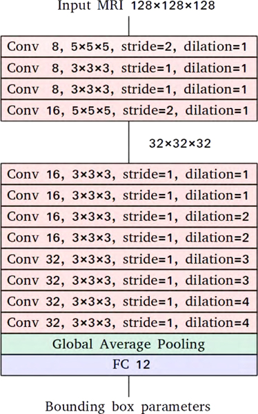
We used downsampled MRI images for hemisphere localization to reduce their memory footprint and to speed up the training process. Figure 2 illustrates the architecture of our localization network. It uses convolutional layers with increasing dilation factors. Each convolutional layer is followed by an instance normalization layer and an activation layer with leaky rectified linear units (Ulyanov et al., 2017; Maas et al., 2013). The convolutional layers are followed by a global average pooling layer which performs extreme dimensionality reduction. The final layer is a fully connected layer with 12 units. It performs bounding box regression to predict the center voxel’s coordinates and the bounding box’s dimensions for each hemisphere. The network outputs a total of 12 bounding box parameters for a given image. We trained the network to minimize the mean squared error using the Adam optimization method with the default learning rate of 0.001 and a batch size of 8 (Kingma and Ba, 2014). For augmentation, we applied translation of maximum 20 voxels on-the-fly.
Figure 2:
The localization network predicts the coordinates of the center voxel and the width, the height, and the depth of the bounding box for each hemisphere. Each block in the figure listed the detailed parameters for each network layer. For the convolutional layer (red), parameters include: the number of convolutional filters, convolutional kernel size, stride number, and dilation sizes; the global average polling layer (green) doesn’t include learnable parameters; the fully connected layer have output a total of 12 parameters representing the coordination for the two bounding boxes for each given image (6 for each hemisphere).
3.2. Segmentation network
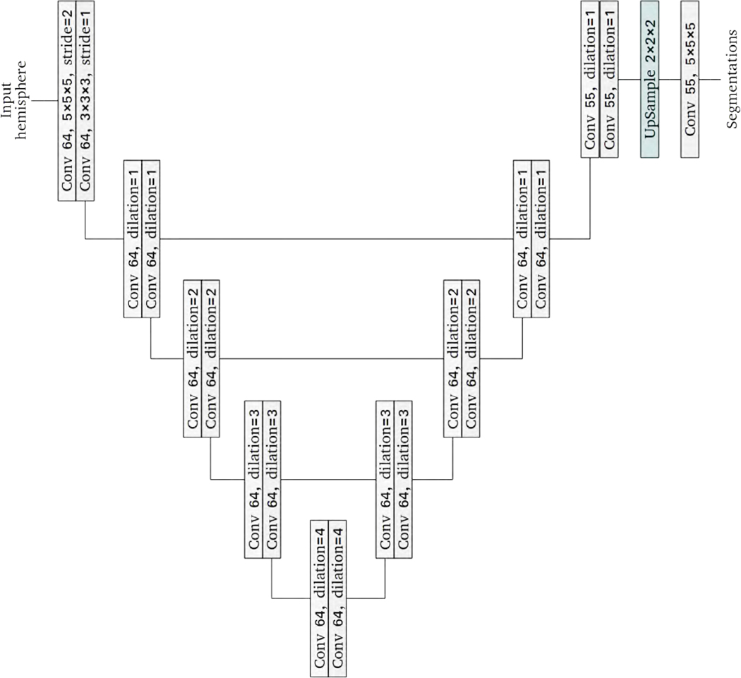
Our segmentation network is shown in Figure 3. Similarly to the popular U-Net architecture, our network has two paths of convolutional networks with skip connections between the paths to promote information flow (Ronneberger et al., 2015). The skip connections simply concatenate features in one path to those in the other path. However, unlike the U-Net architecture, we did not perform downsampling and upsampling in the two paths. Rather, we progressively increased the dilation factors in one path and decreased the dilation factors in the other path. Increasing the dilation factors expands the receptive field size, providing more spatial context to subsequent network layers. While a large dilation factor is useful for the global context, it can be detrimental to small regions with thin boundaries. In the other path, we used decreasing dilation factors to aggregate local features. Similar networks have been used to segment small objects in remote sensing tasks (Hamaguchi et al., 2018). We only performed downsampling in the first layer to reduce the input image’s size and memory usage. With the exception of the final layer, every convolutional layer is followed by an instance normalization layer and an activation layer with leaky rectified linear units (Ulyanov et al., 2017; Maas et al., 2013). In total, the network has 21 convolutional layers.
Figure 3:
The architecture of the proposed segmentation network. Each block in the figure listed the detailed parameters for the corresponding network layer. Each convolution layer uses a kernel size of 3 × 3 × 3, a stride of 1 × 1 × 1 and a dilation factor of 1 unless otherwise specified.
We trained the network to minimize both the voxel-wise cross-entropy loss and the soft dice loss according to:
The soft dice loss for each region is given by
where the sums run over N voxels of a predicted segmentation and a reference segmentation y. The final soft dice loss is the average of the soft dice losses of all regions. Since the cross-entropy loss function treats all voxels equally and independently evaluates the class prediction for each voxel, networks trained using only the cross-entropy loss function fail to detect small regions. Therefore, the network would be biased towards regions with large volumes. On the other hand, the soft dice loss function implicitly re-weighs the voxels, which helps handle such class imbalances. However, since this function does not differentiate between over-segmentation and under-segmentation, we opted to optimize both cross-entropy and soft dice loss. We trained the network using the Adam optimization method with the default learning rate of 0.001 (Kingma and Ba, 2014). We used 2 GPUs to speed up the training process, with each GPU processing one hemisphere. We stopped training the network when the validation loss stopped decreasing. In total, we trained the network for 12 epochs which took about 72 hours.
Table 2 listed the configuration details for both of the hemisphere localization and the segmentation networks, including the number of trainable parameters, number of epochs, optimizer, batch size, and the loss function.
Table 2:
Configuration details for both of the localization and the segmentation networks, including: Number of trainable parameters, number of epochs, optimizer, batch size, and the loss function.
| Localization network | Segmentation network | |
|---|---|---|
| Trainable parameters | 145k | 1.1M |
| Epochs | 12 | 12 |
| Optimizer | Adam | Adam |
| learning rate | 0.001 | 0.001 |
| Batch size | 8 | 1 |
| Loss | MSE | DiceCE |
Abbreviation: MSE: Mean Squared Error loss; DiceCE: Soft dice loss + Cross Entropy loss.
3.3. Post-processing
To create a final whole-brain segmentation, we used the bounding boxes to orient the two segmentations obtained by passing the left and horizontally flipped right hemispheres to the segmentation network. Since the bounding boxes of the two hemispheres overlap, we used majority voting with a neighborhood for each voxel where the two segmentations disagreed. We combined the left and right labels for 6 structures (white matter hypointensities, 3rd-ventricle, 4th-ventricle, brain stem, corpus callosum and cerebrospinal fluid) and kept the left and right labels separate for the remaining 48 structures. The final segmentation had a total of 102 structures. We computed a brain mask by performing dilation and keeping the largest component. The brain mask was used to convert the labels of any voxels located outside of the brain to background.
3.4. Evaluation measures
We used three metrics to analyze the similarity and discrepancy between our segmentation and a reference segmentation: signed relative volume difference (SRVD), Dice Similarity Coefficient (DSC) and Hausdorff Distance (HD). SRVD is computed according to:
where A is a binary reference segmentation and B is a predicted segmentation. It is a volume-based metric that ranges between −100 and 100, where 0 indicates perfect segmentation, positive value indicates over-segmentation, and negative value indicates under-segmentation. Note that imperfect segmentations or even non-overlapping segmentations can result in a SRVD of 0 as long as the volumes of the predicted and reference segmentations are equal. In our variant of SRVD, we ignore the direction of volume difference and take the absolute of relative volume difference (ARVD) according to:
where and are segmentations of the first and second scans of a pair of back-to-back scans. This metric measures the variability of volume measurements for scans acquired on the same day.
We used DSC to measure overlap (Dice, 1945). It provides a similarity measure that ranges between 0 and 1, where 0 shows no overlap between two segmentations and 1 shows 100% overlap. DSC is defined as the following
For small structures, DSC may be overly sensitive to errors. Note that DSC does not differentiate between over-segmentation and under-segmentation, nor does it account for shape fidelity.
HD, a distance-based metric, measures the discrepancy between two shapes (Jain and Dubes, 1988). It is defined by
where is computed according to
HD compares the boundaries between two segmentations and gives the maximum of all distances from a boundary point in one segmentation to the closest boundary point in the other segmentation. A low HD value indicates that every point of either segmentation is close to some point of the other segmentation. Note that HD is sensitive to outliers and a single outlying voxel can result in a high HD value.
4. Results
4.1. Localization performance
In Table 3, we show the performance of the localization network on the held-out test data. Overall, each predicted coordinate is within 3 voxels away from the ground truth coordinate, and each predicted dimension is within 4 voxels of size difference. To account for error in the localization network and to avoid under-segmentation, we increased each predicted dimension of the bounding boxes by 10 voxels. The expanded bounding boxes were used to localize both hemispheres in the segmentation network.
Table 3:
Mean and standard deviation of the absolute difference between the predicted and ground truth bounding box parameters.
| Hemisphere | Coordinates of center voxel | Width | Height | Depth | ||
|---|---|---|---|---|---|---|
| x | y | z | ||||
|
| ||||||
| Left | 1.472 1.189 | 2.695 1.888 | 2.000 1.748 | 2.566 2.148 | 1.535 1.235 | 2.140 1.735 |
| Right | 1.060 0.949 | 2.690 1.855 | 1.907 1.719 | 2.483 1.994 | 1.532 1.226 | 2.179 1.785 |
4.2. Evaluation of segmentation accuracy
4.2.1. Held-out test data
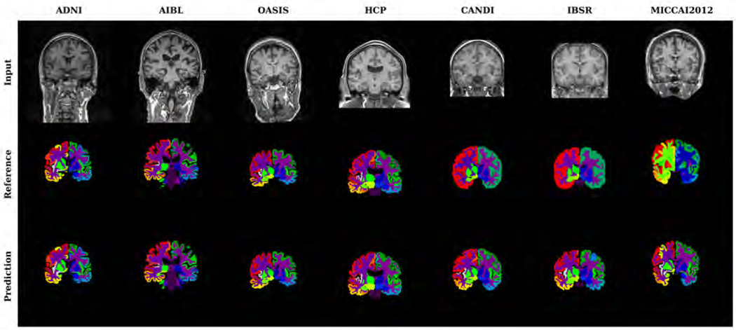
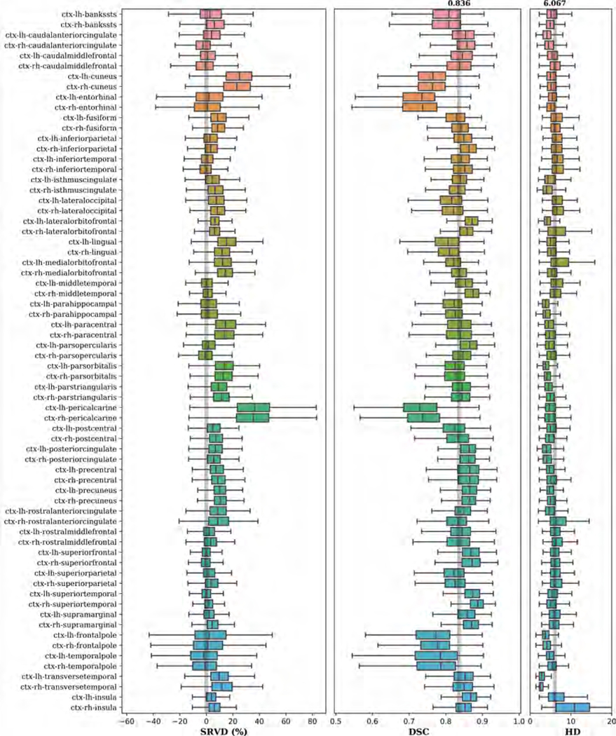
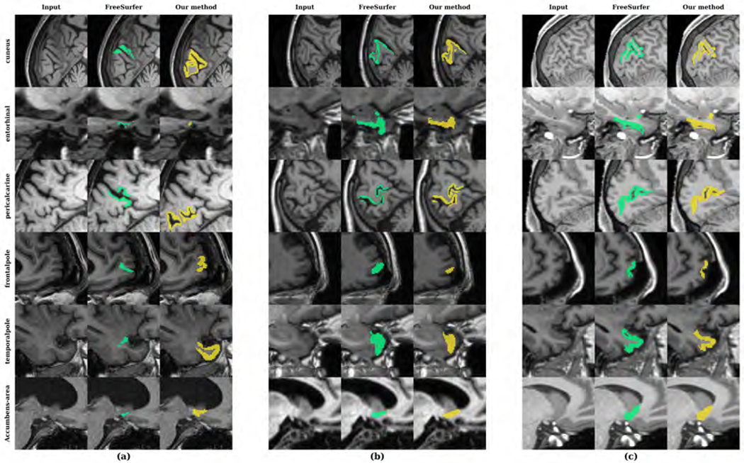
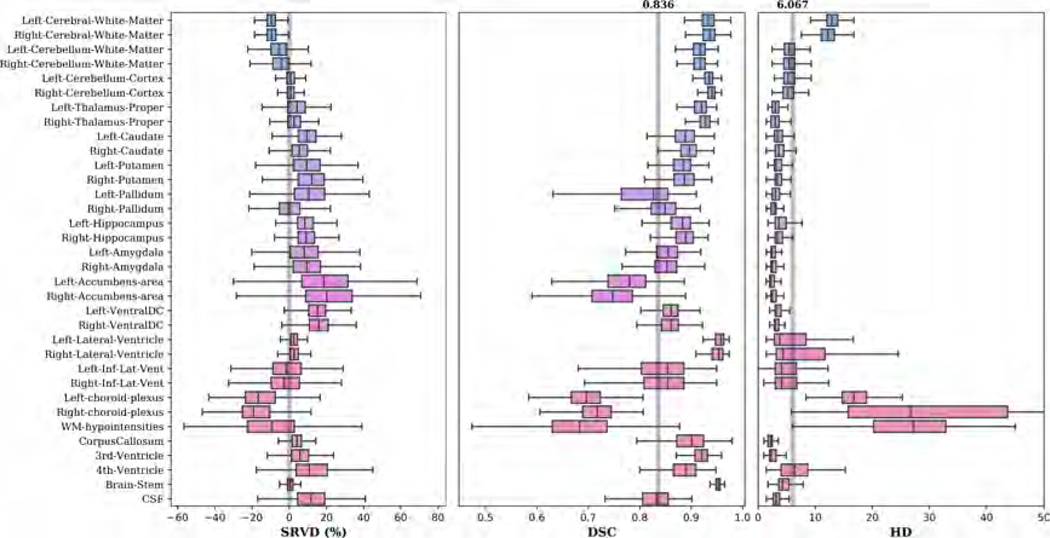
Figure 4 shows examples of input images, reference segmentations, and our automatic segmentations. For the held-out test data, the distributions of SRVD, DSC and HD for all structures are shown in Figure 5. The overall mean DSC is 0.836 and the overall mean HD is 6.067. Regions with a mean DSC that is much lower than the overall mean DSC include bilateral cuneus, entorhinal, pericalcarine, frontal pole, temporal pole, and accumbens areas. The errors in these regions are likely due to over-segmentation as the predicted volumes of these regions tended to be higher than the reference volumes. However, over-segmentation errors are mostly limited since the distances between the predicted boundaries and the reference boundaries of these structures are quite small, as shown in the HD boxplot. We show sample segmentations of these regions in Figure 7. The first column shows that the FreeSurfer segmentations are not error-free, potentially resulting in low DSC values for some images. The bilateral choroid plexus and white matter hypointensities regions include scattered voxels, making their DSC and HD metrics much more sensitive to errors and outliers.
Figure 4:
Examples of test input images, reference segmentations, and predicted segmentations. Reference segmentation refers to FreeSurfer segmentation except for the CANDI, IBSR and MICCAI 2012 datasets, in which case it refers to manual segmentation.
Figure 5:
Boxplots of SRVD, DSC and HD for 68 cortical structures evaluated on the held-out test data. For the SRVD boxplot, a gray line is drawn on the reference point 0. The gray lines in the DSC and HD boxplots show the overall mean DSC and HD values across all structures.
Figure 7:
Sample segmentations of the held-out test dataset with the (a) lowest, (b) median and (c) highest DSC in bilateral cuneus, entorhinal, pericalcarine, frontal pole and temporal pole.
4.3. Comparison with manual segmentation
The manual segmentations provided in the CANDI, IBSR and MICCAI 2012 data sets contained different numbers of structures, some of which do not directly correspond to any FreeSurfer label. However, all three data sets have manual segmentations of the subcortical structures. For this experiment, we focused on comparing our automatic subcortical segmentation results with these manual subcortical segmentations.
4.3.1. CANDI dataset
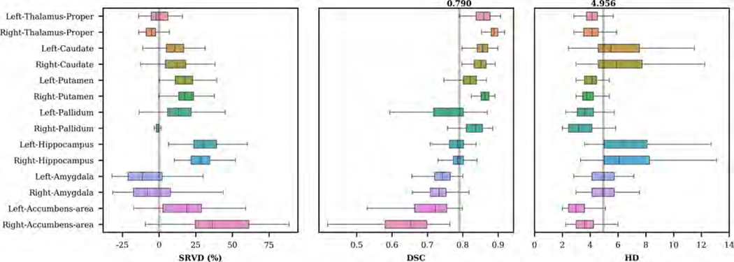
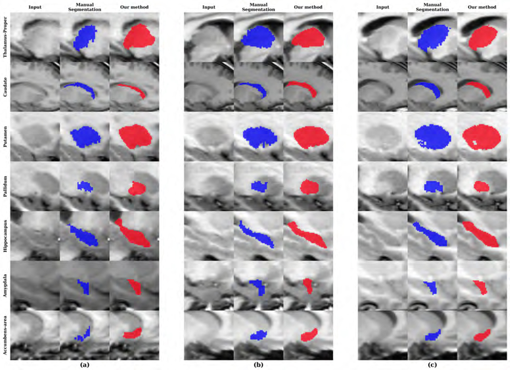
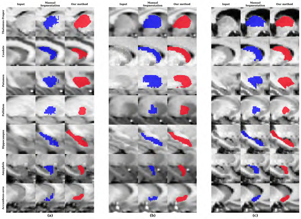
We evaluated our network on the CANDI dataset. In Figure 8, we show the distribution of SRVD, DSC and HD for several subcortical regions. The mean DSC is 0.79. DSC scores greater than 0.85 were observed in the bilateral thalamus, bilateral caudate and right putamen, while lower DSC scores were observed in the bilateral amygdala and accumbens areas. The volume difference boxplot indicates that our network tends to over-segment most of the subcortical regions except for the amygdala. A challenging aspect of the CANDI data set is that it represents a much younger demographic. Overall, the distances between the predicted and reference boundaries were quite small except for bilateral caudate and hippocampus. For each subcortical region, we show examples of the input images and segmentations in Figure 9.
Figure 8:
Boxplots of SRVD, DSC and HD for 14 subcortical structures evaluated on the CANDI dataset. For the SRVD boxplot, a gray line is drawn on the reference point 0. The gray lines in the DSC and HD boxplots show the overall mean DSC and HD values across all structures.
Figure 9:
Sample segmentations of the CANDI dataset with the (a) lowest, (b) median and (c) highest DSC for each subcortical region.
4.3.2. IBSR dataset
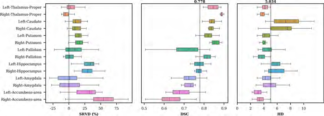
Figure 10 shows the distributions of SRVD, DSC and HD for the 14 subcortical structures obtained on the IBSR dataset. Overall, the predicted subcortical volumes are higher than the volumes derived from manual segmentations. The overall mean DSC is 0.778. Larger structures such as the thalamus, caudate, and putamen have higher DSC values, whereas smaller structures such as the amygdala and accumbens area have lower DSC values. The overall mean HD is 5.034. Regions with mean HD larger than the overall mean include bilateral caudate and hippocampus.
Figure 10:
Boxplots of SRVD, DSC and HD for 14 subcortical structures evaluated on the IBSR dataset. For the SRVD boxplot, a gray line is drawn on the reference point 0. The gray lines in the DSC and HD boxplots show the overall mean DSC and HD values across all structures.
We compared our method with the state-of-the-art methods in Table 4. For a fair comparison, we included only methods that performed independent testing on the IBSR data set. The overall mean DSC and HD achieved using our network were 0.779 and 5.034. Even though our network was trained on FreeSurfer data, it performed better on the IBSR data compared to the FreeSurfer data. The performance of our network is also comparable with other CNN-based approaches (Dolz et al., 2018; Roy et al., 2018). However, these networks were trained to segment much smaller numbers of structures. Dolz et al. (2018) trained their network to segment 8 subcortical structures and Roy et al. (2018) fined-tuned their network with other manual segmentations to segment 27 structures. We show samples of IBSR images and their segmentations in Figure 11 to highlight the fact that these images have a lower contrast and a lower resolution of 1.5 mm in the anterior-posterior direction, which make these images difficult to segment.
Table 4:
Comparison of performances achieved on the IBSR dataset via independent testing.
| Structure | FreeSurfer | Dolz et al. (2018) | Roy et al. (2018) | Our method | ||
|---|---|---|---|---|---|---|
| DSC | HD | DSC | DSC | DSC | HD | |
| Thalamus-Proper (L) Thalamus-Proper (R) |
0.815 0.056 0.864 0.022 |
5.367 1.168 4.471 1.245 |
0.87 | 0.87 | 0.845 0.029 0.889 0.008 |
4.263 0.610 3.703 0.482 |
| Caudate (L) Caudate (R) |
0.796 0.050 0.809 0.048 |
6.435 1.939 8.201 2.443 |
0.84 | 0.86 | 0.833 0.038 0.832 0.030 |
7.322 2.298 6.905 2.014 |
| Putamen (L) Putamen (R) |
0.789 0.038 0.829 0.031 |
5.310 0.923 4.716 1.189 |
0.85 | 0.88 | 0.819 0.027 0.857 0.019 |
4.542 1.169 4.105 0.447 |
| Pallidum (L) Pallidum (R) |
0.632 0.171 0.774 0.032 |
4.652 1.294 3.966 0.793 |
0.79 | 0.81 | 0.709 0.083 0.812 0.033 |
4.871 1.196 3.677 0.613 |
| Hippocampus (L) | 0.760 0.036 | 5.787 1.264 | - | - | 0.774 0.028 | 6.069 1.217 |
| Hippocampus (R) | 0.767 0.060 | 5.615 1.600 | - | - | 0.774 0.030 | 9.204 7.121 |
| Amygdala (L) | 0.661 0.069 | 5.521 1.517 | - | - | 0.723 0.051 | 4.646 1.234 |
| Amygdala (R) | 0.690 0.067 | 4.720 1.553 | - | - | 0.717 0.055 | 5.042 1.571 |
| Accumbens-area (L) | 0.604 0.071 | 3.634 0.783 | - | - | 0.679 0.065 | 3.155 0.599 |
| Accumbens-area (R) | 0.574 0.074 | 4.507 1.077 | - | - | 0.631 0.067 | 3.463 0.652 |
|
| ||||||
| Average | 0.740 0.110 | 5.207 1.761 | - | - | 0.778 0.086 | 5.034 1.582 |
Figure 11:
Sample segmentations of the IBSR dataset with the (a) lowest, (b) median and (c) highest DSC for each subcortical region.
4.3.3. MICCAI 2012 Multi-Atlas dataset
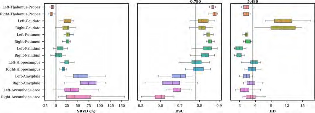
We show the distributions of SRVD, DSC and HD obtained on the MICCAI 2012 dataset in Figure 12. The overall mean DSC was 0.780 and the DSC values for bilateral amygdala and accumbens area were the lowest. The overall HD was 5.486 and the HD values for bilateral caudate were the worst. In Figure 13, we show examples of caudate segmentations sorted by HD values and we show examples of amygdala and accumbens area segmentations sorted by DSC values. Table 5 compares the DSC and HD values obtained using our method and FreeSurfer. Our method showed a significant improvement of segmentation accuracy for most of the structures, except for the caudate and hippocampus. Other CNN-based methods have shown lower to comparable performances prior to training on the MICCAI 2012 images and higher performances after training on the MICCAI 2012 images (Roy et al., 2018; Kushibar et al., 2018).
Figure 12:
Boxplots of SRVD, DSC and HD for 14 subcortical structures evaluated on the MICCAI 2012 dataset. For the SRVD boxplot, a gray line is drawn on the reference point 0. The gray lines in the DSC and HD boxplots show the overall mean DSC and HD values across all structures.
Figure 13:
Sample segmentations of the MICCAI 2012 dataset with the (a) worst, (b) median and (c) best HD values for caudate and DSC values for other structures.
Table 5:
Comparison of performances achieved on the MICCAI 2012 dataset using our method and FreeSurfer. The p-value showed the statistical results of the repeated-measures t-test, indicating a significant improvement of segmentation accuracy for most of the structures, except for the caudate and hippocampus.
| Structure | FreeSurfer | Our method | p-value | |||
|---|---|---|---|---|---|---|
| DSC | HD | DSC | HD | DSC | HD | |
| Thalamus-Proper (L) | 0.830 0.018 | 4.94 1.01 | 0.866 0.011 | 4.44 0.95 | 0.000 | 0.037 |
| Thalamus-Proper (R) | 0.849 0.021 | 4.76 0.75 | 0.876 0.012 | 4.38 0.71 | 0.000 | 0.033 |
| Caudate (L) | 0.808 0.079 | 9.89 3.09 | 0.810 0.051 | 11.35 2.40 | 0.900 | 0.031 |
| Caudate (R) | 0.801 0.042 | 10.39 3.09 | 0.810 0.039 | 11.01 2.62 | 0.356 | 0.368 |
| Putamen (L) | 0.771 0.039 | 6.31 1.09 | 0.843 0.019 | 4.45 0.78 | 0.000 | 0.000 |
| Putamen (R) | 0.799 0.026 | 5.85 0.84 | 0.849 0.023 | 4.57 0.78 | 0.000 | 0.000 |
| Pallidum (L) | 0.693 0.189 | 3.89 1.07 | 0.837 0.033 | 2.98 0.73 | 0.000 | 0.000 |
| Pallidum (R) | 0.792 0.085 | 3.45 0.98 | 0.821 0.049 | 2.96 0.54 | 0.085 | 0.012 |
| Hippocampus (L) | 0.784 0.054 | 6.35 1.87 | 0.779 0.041 | 6.16 1.66 | 0.664 | 0.654 |
| Hippocampus (R) | 0.794 0.025 | 6.19 1.59 | 0.794 0.035 | 5.66 1.54 | 1.000 | 0.161 |
| Amygdala (L) | 0.585 0.064 | 5.05 0.97 | 0.694 0.050 | 4.38 1.02 | 0.000 | 0.006 |
| Amygdala (R) | 0.576 0.076 | 5.43 0.90 | 0.661 0.065 | 5.17 1.00 | 0.000 | 0.257 |
| Accumbens-area (L) | 0.630 0.055 | 4.28 1.11 | 0.683 0.053 | 4.07 1.08 | 0.000 | 0.425 |
| Accumbens-area (R) | 0.443 0.065 | 5.47 1.02 | 0.592 0.061 | 5.23 1.03 | 0.000 | 0.331 |
|
| ||||||
| Average | 0.725 0.137 | 5.87 2.48 | 0.780 0.094 | 5.49 2.82 | 0.054 | 0.551 |
4.4. Evaluation of segmentation consistency
4.4.1. MIRIAD dataset
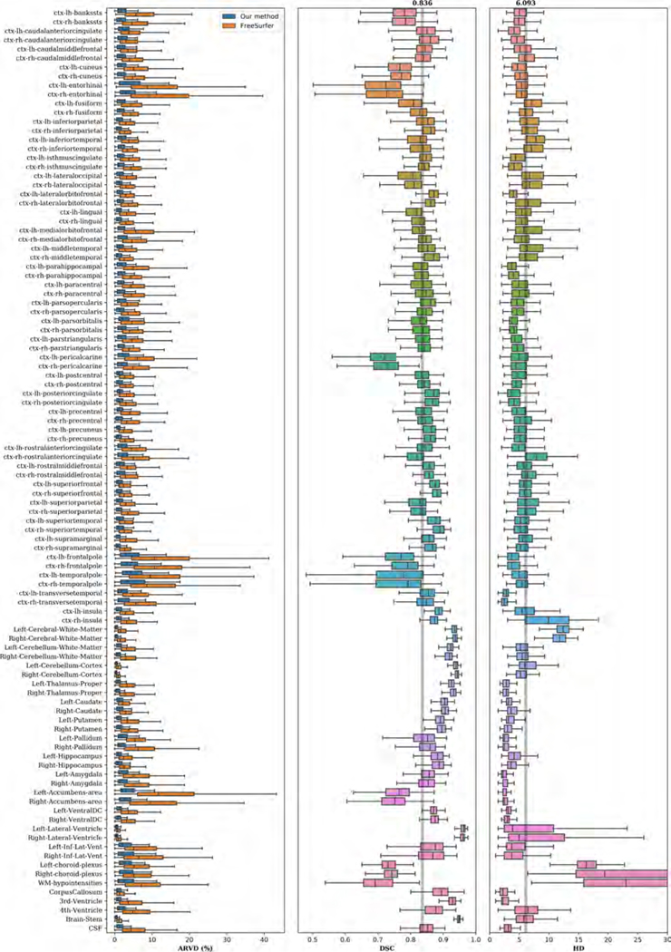
The DSC and HD distribution patterns in Figure 14 are similar to those of the held-out test data with an overall mean DSC of 0.836 and HD of 6.093 across 102 structures. The overall mean change in volumes across back-to-back scans is 2.229 for our method and 5.634 for FreeSurfer. This indicates that our network is capable of generating consistent segmentations and volume measurements for intra-session scans.
Figure 14:
Boxplots of ARVD, DSC and HD for 102 structures evaluated on the MIRIAD dataset. The ARVD boxplot shows the variability of volumetric measurements across back-to-back scans. The gray lines in the DSC and HD boxplots show the overall mean DSC and HD values across all structures.
4.4.2. TRT dataset
We computed the intra-session coefficient of variation where the standard deviation of intra-session measurements, , is based on differences between pairs of back-to-back measurements (Maclaren et al., 2014). The total coefficient of variation, , was computed using the standard deviation across all measurements. Table 6 shows the comparison between the intra-session and total variation of volumetric measurements of subcortical structures obtained using our method and FreeSurfer. The volumetric measurements generated using our method have less variation between scans and days.
Table 6:
Comparison of intra-session () and total variation () of volumetric measurements obtained on the TRT dataset using our method and FreeSurfer.
| Structure | FreeSurfer | Our method | ||||
|---|---|---|---|---|---|---|
| Mean volume (ml) | (intra-session) | (total) | Mean volume (ml) | (intra-session) | (total) | |
| Thalamus | 12.90 | 5.98 | 6.06 | 14.51 | 1.51 | 1.76 |
| Caudate | 7.40 | 1.54 | 1.58 | 7.75 | 0.63 | 0.71 |
| Putamen | 11.60 | 4.04 | 3.92 | 10.73 | 1.04 | 1.22 |
| Pallidum | 3.20 | 5.25 | 5.42 | 3.17 | 2.26 | 2.56 |
| Hippocampus | 8.90 | 2.77 | 2.92 | 9.19 | 0.83 | 0.95 |
| Amygdala | 3.80 | 4.69 | 5.21 | 3.07 | 1.18 | 1.49 |
5. Discussion
In this study, We proposed a new strategy for whole-brain segmentation, in which a CNN is first trained on both the left and horizontally flipped right hemispheres rather than smaller patches. A hemisphere can be considered as a very large patch that contains all the structures to be segmented. This provides an important context for the segmentation task and simplifies the sampling process for network training. A patch-based CNN requires a more sophisticated sampling strategy that accounts for the presence of brain structures in each patch. The localization network can therefore be considered as part of a sampling strategy. Additionally, using a hemisphere as the input patch allows us to more efficiently learn representations and manage memory usage. We can use the same representations for both hemispheres by simply performing a left-right flip on one of the hemispheres. In other words, our segmentation network does not need to learn separate filters and generate separate labels for the left and right parts of each structure. The predicted segmentations can be affixed with left and right annotations based on which bounding box was used. Since each hemisphere is considered as an independent sample, this strategy also allows us to double the number of training samples.
Our method shows high accuracy in generating FreeSurfer segmentations as shown in Section 4.2.1. However, it is difficult to directly compare our method with other CNN approaches due to differences in the selection of training data, testing data and brain structures. The experiment most closely related ours, McClure et al. (2018), trained a patch-based CNN (323 patches) on a very large dataset (N = 11,148) to generate FreeSurfer-based segmentations of 49 brain structures. They achieved a DSC of 0.78 on a held-out test data and a DSC of 0.73 on an independent test data. Our network, which obtained DSC of 0.836 on both the held-out test data and independent MIRIAD data, outperformed their CNN. In comparing our segmentations with manual segmentations, we have demonstrated that our network’s subcortical segmentation performance is comparable to other CNN-based approaches. On intra-session scans, our method showed consistent volumetric measurements.
In addition to the improvement in terms of accuracy, the proposed method also showed improvement in computational complexity and reduction in the inference time. In terms of computational complexity, the light-weight hemisphere localization network is able to reduce the input image dimension to half of the original size. Furthermore, the proposed framework is able to drastically reduce the whole brain segmentation time from FreeSurfer’s over 24 hours to the level of seconds. In addition, compared to the other CNN-based whole brain segmentation using multi-view 2D slices as input and using sliding windows during inference(Roy et al., 2019; Henschel et al., 2020), the proposed hemisphere-based 3D-CNN segmentation is able to achieve further speedup the segmentation at given that only two forward passes are necessary to perform inference on each volume.
5.1. Limitations and future work
We note that our method performed better on images with similar acquisition parameters as the training data. To generalize better to unseen data, our network needs to be more robust to intensity, contrast and scanner variations. We used minimal pre-processing, augmentation, and post-processing techniques in our experiments. Pre-processing techniques such as intensity, contrast and spatial normalization are often performed to provide segmentation algorithms with consistent input images. Alternatively, augmentation strategies such as alteration of the intensity and contrast in training images can be employed to expose our segmentation network to a wider range of images. A recent study showed that augmenting the contrast in training images can improve the robustness of segmentation networks (Jog et al., 2019). This augmentation scheme uses altered versions of training images to simulate various acquisition protocols. A network trained on voxel-wise cross-entropy loss and soft Dice loss does not actually learn inter-class relationship, and it does not account for the topological interactions of different structures. This may lead to implausible classifications. Various studies have used fully connected conditional random fields while post-processing their results to formulate constraints among voxels and penalize implausible connections among voxel pairs (Wachinger et al., 2018; Kamnitsas et al., 2017; Chen et al., 2014). Some of these techniques can improve our network’s robustness and performance.
Finally, in this study, we have tested the robustness of the proposed whole brain segmentation through extensive independent validation of the proposed methods using multiple independent dataset, including CANDI, IBSR, and MICCAI2012. To translate the proposed machine-learning-based method into a real clinical situation, further extensive clinical evaluations with perspective studies on independent real clinical institutional datasets are necessary (Ma et al., 2021). The clinical generalizability of the proposed model could potentially be further improved by incorporating more divesed dataset collected from multiple sites with different clinical situations. On the other hand, challenges are still needed to be resolved. For example, additional manual ground truth data would be expensive to generate, even through semi-automatic procedures using the constantly evolving segmentation model. And the constrain of limited capability of sharing privacy-sensitive patient data might need to be overcome through federated learning approaches (Lo et al., 2021).
6. Conclusions
We have presented a CNN-based segmentation strategy that performs segmentation directly on large and semantically meaningful input images. We trained our neural networks to localize and segment cerebral hemispheres. Through various experiments, our network demonstrated high accuracy in generating FreeSurfer-based segmentations, outperformed FreeSurfer in subcortical segmentations of the IBSR and MICCAI 2012 datasets, and produced consistent volumetric measurements for intra-session scans.
Figure 6:
Boxplots of SRVD, DSC and HD for 34 subcortical structures evaluated on the held-out test data. For the SRVD boxplot, a gray line is drawn on the reference point 0. The gray lines in the DSC and HD boxplots show the overall mean DSC and HD values across all structures.
Acknowledgments
This work was supported by Natural Sciences and Engineering Research Council (NSERC), Canadian Institutes of Health Research (CIHR), Michael Smith Foundation for Health Research (MSFHR), Brain Canada, the Pacific Alzheimer Research Foundation (PARF), Alzheimer Society of Canada (Alzheimer Society Research Program), and the National Institute on Aging (R01 AG055121). There is no conflict of interest to declare from all authors. We thank Compute Canada for providing the computational infrastructure used in this study.
Data collection and sharing for this project was funded by the Alzheimer’s Disease Neuroimaging Initiative (ADNI) (National Institutes of Health Grant U01 AG024904) and DOD ADNI (Department of Defense award number W81XWH-122-0012). ADNI is funded by the National Institute on Aging, the National Institute of Biomedical Imaging and Bioengineering, and through generous contributions from the following: AbbVie, Alzheimer’s Association; Alzheimer’s Drug Discovery Foundation; Araclon Biotech; BioClinica, Inc.; Biogen; Bristol-Myers Squibb Company; CereSpir, Inc.;Cogstate;Eisai Inc.; Elan Pharmaceuticals, Inc.; Eli Lilly and Company; EuroImmun; F. Hoffmann-La Roche Ltd and its affiliated company Genentech, Inc.; Fujirebio; GE Healthcare; IXICO Ltd.; Janssen Alzheimer Immunotherapy Research & Development, LLC.; Johnson & Johnson Pharmaceutical Research & Development LLC.; Lumosity; Lundbeck; Merck & Co., Inc.; Meso Scale Diagnostics, LLC.;NeuroRx Research; Neurotrack Technologies;Novartis Pharmaceuticals Corporation; Pfizer Inc.; Piramal Imaging; Servier; Takeda Pharmaceutical Company; and Transition Therapeutics.The Canadian Institutes of Health Research is providing funds to support ADNI clinical sites in Canada. Private sector contributions are facilitated by the Foundation for the National Institutes of Health (www.fnih.org). The grantee organization is the Northern California Institute for Research and Education, and the study is coordinated by the Alzheimer’s Therapeutic Research Institute at the University of Southern California. ADNI data are disseminated by the Laboratory for Neuro Imaging at the University of Southern California.
Training data were provided by OASIS (Principal Investigators: T. Benzinger, D. Marcus, J. Morris). The OASIS-3 project was supported by the following grants: NIH P50AG00561, P30NS098577 P01AG026276, P01AG003991, R01AG043434, UL1TR000448, and R01EB009352. Data were provided [in part] by the Human Connectome Project, WU-Minn Consortium (Principal Investigators: David Van Essen and Kamil Ugurbil; 1U54MH091657) funded by the 16 NIH Institutes and Centers that support the NIH Blueprint for Neuroscience Research; and by the McDonnell Center for Systems Neuroscience at Washington University Independent testing data used in the preparation of this article were also obtained from the MIRIAD database. The MIRIAD investigators did not participate in analysis or writing of this report. The MIRIAD dataset is made available through the support of the UK Alzheimer’s Society (Grant RF116). The original data collection was funded through an unrestricted educational grant from GlaxoSmithKline (Grant 6GKC).
Footnotes
Data used in preparation of this article were obtained from the Alzheimer’s Disease Neuroimaging Initiative (ADNI) database (http://adni.loni.usc.edu). As such, the investigators within the ADNI contributed to the design and implementation of ADNI and/or provided data but did not participate in analysis or writing of this report. A complete listing of ADNI investigators can be found at: http://adni.loni.usc.edu/wp-content/uploads/how_to_apply/ADNI_Acknowledgement_List.pdf
Data used in the preparation of this article was obtained from the Australian Imaging Biomarkers and Lifestyle flagship study of ageing (AIBL) funded by the Commonwealth Scientific and Industrial Research Organisation (CSIRO) which was made available at the ADNI database (www.loni.usc.edu/ADNI). The AIBL researchers contributed data but did not participate in the analysis or writing of this report. AIBL researchers are listed at www.aibl.csiro.au
Declaration of interests
The authors declare that they have no known competing financial interests or personal relationships that could have appeared to influence the work reported in this paper.
Evangeline Yee: Methodology, Software, Validation, Formal analysis, Data curation, Visualization, Writing - Original Draft
Da Ma: Methodology, Software, Validation, Formal analysis, Investigation, Data curation, Visualization, Project administration, Writing - Original Draft, Review & Editing
Karteek Popuri: Software, Project administration, Investigation, Data curation,
Shuo Chen: Software, Validation, Formal analysis
Hyunwoo Lee: Investigation, Validation, Writing - Review & Editing
Vincent Chow: Data curation, Project administration
Cydney Ma: Data curation, Project administration
Lei Wang: Conceptualization, Resources, Supervision, Funding acquisition, Writing - Review & Editing
Mirza Faisal Beg: Conceptualization, Resources, Supervision, Funding acquisition, Writing - Review & Editing
Publisher's Disclaimer: This is a PDF file of an unedited manuscript that has been accepted for publication. As a service to our customers we are providing this early version of the manuscript. The manuscript will undergo copyediting, typesetting, and review of the resulting proof before it is published in its final form. Please note that during the production process errors may be discovered which could affect the content, and all legal disclaimers that apply to the journal pertain.
References
- Agosta F, Galantucci S, Filippi M, 2017. Advanced magnetic resonance imaging of neurodegenerative diseases. Neurological Sciences 38, 41–51. doi: 10.1007/s10072-016-2764-x. [DOI] [PubMed] [Google Scholar]
- de Brebisson A, Montana G, 2015. Deep neural networks for anatomical brain segmentation, in: Proceedings of the IEEE Conference on Computer Vision and Pattern Recognition Workshops, pp. 20–28. [Google Scholar]
- Chen LC, Papandreou G, Kokkinos I, Murphy K, Yuille AL, 2014. Semantic image segmentation with deep convolutional nets and fully connected crfs. arXiv preprint arXiv:1412.7062. [DOI] [PubMed] [Google Scholar]
- Derakhshan M, Caramanos Z, Giacomini PS, Narayanan S, Maranzano J, Francis SJ, Arnold DL, Collins DL, 2010. Evaluation of automated techniques for the quantification of grey matter atrophy in patients with multiple sclerosis. NeuroImage 52, 1261–1267. doi: 10.1016/j.neuroimage.2010.05.029. [DOI] [PubMed] [Google Scholar]
- Despotović I, Goossens B, Philips W, 2015. MRI Segmentation of the Human Brain: Challenges, Methods, and Applications. Computational and Mathematical Methods in Medicine 2015, 450341. URL: 10.1155/2015/450341, doi: 10.1155/2015/450341. [DOI] [PMC free article] [PubMed] [Google Scholar]
- Dice LR, 1945. Measures of the amount of ecologic association between species. Ecology 26, 297–302. [Google Scholar]
- Dolz J, Desrosiers C, Ayed IB, 2018. 3d fully convolutional networks for subcortical segmentation in mri: A large-scale study. NeuroImage 170, 456–470. [DOI] [PubMed] [Google Scholar]
- Ellis KA, Bush AI, Darby D, De Fazio D, Foster J, Hudson P, Lauten-schlager NT, Lenzo N, Martins RN, Maruff P, et al. , 2009. The australian imaging, biomarkers and lifestyle (aibl) study of aging: methodology and baseline characteristics of 1112 individuals recruited for a longitudinal study of alzheimer’s disease. International Psychogeriatrics 21, 672–687. [DOI] [PubMed] [Google Scholar]
- Fedorov A, Damaraju E, Calhoun V, Plis S, 2017. Almost instant brain atlas segmentation for large-scale studies. arXiv preprint arXiv:1711.00457 [Google Scholar]
- Fischl B, 2012. Freesurfer. Neuroimage 62, 774–781. [DOI] [PMC free article] [PubMed] [Google Scholar]
- Fischl B, Salat DH, Busa E, Albert M, Dieterich M, Haselgrove C, Van Der Kouwe A, Killiany R, Kennedy D, Klaveness S, Montillo A, Makris N, Rosen B, Dale AM, Kouwe AVD, Killiany R, Kennedy D, Klaveness S, Montillo A, Makris N, Rosen B, Dale AM, Van Der Kouwe A, 2002. Whole brain segmentation: automated labeling of neuroanatomical structures in the human brain. Neuron 33, 341–55. URL: http://www.ncbi.nlm.nih.gov/pubmed/11832223, doi: 10.1016/S0896-6273(02)00569-X. [DOI] [PubMed] [Google Scholar]
- Fjell AM, Grydeland H, Krogsrud SK, Amlien I, Rohani DA, Ferschmann L, Storsve AB, Tamnes CK, Sala-Llonch R, Due-Tønnessen P, Bjørnerud A, Sølsnes AE, H° aberg AK, Skranes J, Bartsch H, Chen CH, Thompson WK, Panizzon MS, Kremen WS, Dale AM, Walhovd KB, 2015. Development and aging of cortical thickness correspond to genetic organization patterns. Proceedings of the National Academy of Sciences 112, 15462–15467. URL: https://www.pnas.org/content/112/50/15462, doi: 10.1073/pnas.1508831112. [DOI] [PMC free article] [PubMed] [Google Scholar]
- Giedd JN, Snell JW, Lange N, Rajapakse JC, Casey BJ, Kozuch PL, Vaituzis AC, Vauss YC, Hamburger SD, Kaysen D, Rapoport JL, 1996. Quantitative Magnetic Resonance Imaging of Human Brain Development: Ages 4–18. Cerebral Cortex 6, 551–559. URL: 10.1093/cercor/6.4.551, doi: 10.1093/cercor/6.4.551. [DOI] [PubMed] [Google Scholar]
- Gilmore JH, Knickmeyer RC, Gao W, 2018. Imaging structural and functional brain development in early childhood. Nature Reviews Neuroscience 19, 123–137. URL: 10.1038/nrn.2018.1, doi: 10.1038/nrn.2018.1. [DOI] [PMC free article] [PubMed] [Google Scholar]
- Glasser MF, Sotiropoulos SN, Wilson JA, Coalson TS, Fischl B, Andersson JL, Xu J, Jbabdi S, Webster M, Polimeni JR, et al. , 2013. The minimal preprocessing pipelines for the human connectome project. Neuroimage 80, 105–124. [DOI] [PMC free article] [PubMed] [Google Scholar]
- Gogtay N, Giedd JN, Lusk L, Hayashi KM, Greenstein D, Vaituzis AC, Nugent TF, Herman DH, Clasen LS, Toga AW, Rapoport JL, Thompson PM, 2004. Dynamic mapping of human cortical development during childhood through early adulthood. Proceedings of the National Academy of Sciences 101, 8174–8179. URL: https://www.pnas.org/content/101/21/8174, doi: 10.1073/pnas.0402680101. [DOI] [PMC free article] [PubMed] [Google Scholar]
- Grajauskas LA, Siu W, Medvedev G, Guo H, D’Arcy RCN, Song X, 2019. MRI-based evaluation of structural degeneration in the ageing brain: Pathophysiology and assessment. Ageing Research Reviews 49, 67–82. URL: https://www.sciencedirect.com/science/article/pii/S1568163718301119, doi: 10.1016/j.arr.2018.11.004. [DOI] [PubMed] [Google Scholar]
- Gunning-Dixon FM, Brickman AM, Cheng JC, Alexopoulos GS, 2009. Aging of cerebral white matter: a review of MRI findings. International journal of geriatric psychiatry 24, 109–117. URL: https://pubmed.ncbi.nlm.nih.gov/18637641https://www.ncbi.nlm.nih.gov/pmc/articles/PMC2631089/, doi: 10.1002/gps.2087. [DOI] [PMC free article] [PubMed] [Google Scholar]
- Guo H, Siu W, D’Arcy RC, Black SE, Grajauskas LA, Singh S, Zhang Y, Rockwood K, Song X, 2017. MRI assessment of whole-brain structural changes in aging. Clinical interventions in aging 12, 1251–1270. URL: https://pubmed.ncbi.nlm.nih.gov/28848333https://www.ncbi.nlm.nih.gov/pmc/articles/PMC5557118/, doi: 10.2147/CIA.S139515. [DOI] [PMC free article] [PubMed] [Google Scholar]
- Gur RC, Mozley PD, Resnick SM, Gottlieb GL, Kohn M, Zimmerman R, Herman G, Atlas S, Grossman R, Berretta D, 1991. Gender differences in age effect on brain atrophy measured by magnetic resonance imaging. Proceedings of the National Academy of Sciences 88, 2845–2849. URL: https://www.pnas.org/content/88/7/2845, doi: 10.1073/pnas.88.7.2845. [DOI] [PMC free article] [PubMed] [Google Scholar]
- Habibullah H, Albaradie R, Bashir S.a., 2020. MRI Evaluation of Global Developmental Delay: A Retrospective Study. Dubai Medical Journal 3, 1–4. URL: 10.1159/000506900, doi: 10.1159/000506900. [DOI] [Google Scholar]
- Hamaguchi R, Fujita A, Nemoto K, Imaizumi T, Hikosaka S, 2018. Effective use of dilated convolutions for segmenting small object instances in remote sensing imagery, in: 2018 IEEE Winter Conference on Applications of Computer Vision (WACV), IEEE. pp. 1442–1450. [Google Scholar]
- He K, Gkioxari G, Dollár P, Girshick R, 2017. Mask r-cnn, in: Proceedings of the IEEE international conference on computer vision, pp. 2961–2969. [Google Scholar]
- Henschel L, Conjeti S, Estrada S, Diers K, Fischl B, Reuter M, 2020. FastSurfer - A fast and accurate deep learning based neuroimaging pipeline. NeuroImage 219, 117012. URL: 10.1016/j.neuroimage.2020.117012, doi: 10.1016/j.neuroimage.2020.117012, arXiv:1910.03866. [DOI] [PMC free article] [PubMed] [Google Scholar]
- Huo Y, Xu Z, Xiong Y, Aboud K, Parvathaneni P, Bao S, Bermudez C, Resnick SM, Cutting LE, Landman BA, 2019. 3d whole brain segmentation using spatially localized atlas network tiles. NeuroImage 194, 105–119. [DOI] [PMC free article] [PubMed] [Google Scholar]
- Jain AK, Dubes RC, 1988. Algorithms for clustering data. Englewood Cliffs: Prentice Hall, 1988. [Google Scholar]
- Jog A, Hoopes A, Greve DN, Van Leemput K, Fischl B, 2019. Psacnn: Pulse sequence adaptive fast whole brain segmentation. NeuroImage 199, 553–569. [DOI] [PMC free article] [PubMed] [Google Scholar]
- Kamnitsas K, Ledig C, Newcombe VF, Simpson JP, Kane AD, Menon DK, Rueckert D, Glocker B, 2017. Efficient multi-scale 3d cnn with fully connected crf for accurate brain lesion segmentation. Medical image analysis 36, 61–78. [DOI] [PubMed] [Google Scholar]
- Kingma DP, Ba J, 2014. Adam: A method for stochastic optimization. arXiv preprint arXiv:1412.6980. [Google Scholar]
- Knickmeyer RC, Gouttard S, Kang C, Evans D, Wilber K, Smith JK, Hamer RM, Lin W, Gerig G, Gilmore JH, 2008. A structural MRI study of human brain development from birth to 2 years. The Journal of neuroscience : the official journal of the Society for Neuroscience 28, 12176–12182. URL: https://pubmed.ncbi.nlm.nih.gov/19020011https://www.ncbi.nlm.nih.gov/pmc/articles/PMC2884385/, doi: 10.1523/JNEUROSCI.3479-08.2008. [DOI] [PMC free article] [PubMed] [Google Scholar]
- Kushibar K, Valverde S, Gonzalez-Vilĺ a S, Bernal J, Cabezas M, Oliver A, Llado X, 2018. Automated sub-cortical brain structure segmentatioń combining spatial and deep convolutional features. Medical image analysis 48, 177–186. [DOI] [PubMed] [Google Scholar]
- Kuzniecky RI, 1994. Magnetic Resonance Imaging in Developmental Disorders of the Cerebral Cortex. Epilepsia 35, S44–S56. doi: 10.1111/j.1528-1157.1994.tb05988.x. [DOI] [PubMed] [Google Scholar]
- LaMontagne PJ, Keefe S, Lauren W, Xiong C, Grant EA, Moulder KL, Morris JC, Benzinger TL, Marcus DS, 2018. Oasis-3: Longitudinal neuroimaging, clinical, and cognitive dataset for normal aging and alzheimer’s disease. Alzheimer’s & Dementia: The Journal of the Alzheimer’s Association 14, P1097. [Google Scholar]
- Landman B, Warfield S, 2012. Miccai 2012 workshop on multi-atlas labeling, in: Medical image computing and computer assisted intervention conference. [Google Scholar]
- Li W, Wang G, Fidon L, Ourselin S, Cardoso MJ, Vercauteren T, 2017. On the compactness, efficiency, and representation of 3d convolutional networks: brain parcellation as a pretext task, in: International Conference on Information Processing in Medical Imaging, Springer. pp. 348–360. [Google Scholar]
- Liu W, Anguelov D, Erhan D, Szegedy C, Reed S, Fu CY, Berg AC, 2016. Ssd: Single shot multibox detector, in: European conference on computer vision, Springer. pp. 21–37. [Google Scholar]
- Lo J, Yu T, Ma D, Zang P, Owen J, Zhang Q, Wang R, Beg M, Lee A, Jia Y, Sarunic M, 2021. Federated Learning for Microvasculature Segmentation and Diabetic Retinopathy Classification of Optical Coherence Tomography Data. Ophthalmology Science. [DOI] [PMC free article] [PubMed] [Google Scholar]
- Ma D, Cardoso MJ, Modat M, Powell N, Wells J, Holmes H, Wiseman F, Tybulewicz V, Fisher E, Lythgoe MF, Ourselin S, 2014. Automatic Structural Parcellation of Mouse Brain MRI Using Multi-Atlas Label Fusion. PLoS ONE 9, e86576. URL: http://dx.plos.org/10.1371/journal.pone.0086576http://www.pubmedcentral.nih.gov/articlerender.fcgi?artid=3903537&tool=pmcentrez&rendertype=abstract, doi: 10.1371/journal.pone.0086576. [DOI] [PMC free article] [PubMed] [Google Scholar]
- Ma D, Yee E, Stocks JK, Jenkins LM, Popuri K, Chausse G, Wang L, Probst S, Beg MF, 2021. Blinded clinical evaluation for dementia of alzheimer’s type classification using fdg-pet: A comparison between feature-engineered and non-feature-engineered machine learning methods. Journal of Alzheimer’s Disease, 1–12. [DOI] [PMC free article] [PubMed] [Google Scholar]
- Maas AL, Hannun AY, Ng AY, 2013. Rectifier nonlinearities improve neural network acoustic models, in: Proc. icml, p. 3. [Google Scholar]
- Maclaren J, Han Z, Vos SB, Fischbein N, Bammer R, 2014. Reliability of brain volume measurements: A test-retest dataset. Scientific data 1, 140037. [DOI] [PMC free article] [PubMed] [Google Scholar]
- Malone IB, Cash D, Ridgway GR, MacManus DG, Ourselin S, Fox NC, Schott JM, 2013. Miriad—public release of a multiple time point alzheimer’s mr imaging dataset. NeuroImage 70, 33–36. [DOI] [PMC free article] [PubMed] [Google Scholar]
- McClure P, Rho N, Lee JA, Kaczmarzyk JR, Zheng C, Ghosh SS, Nielson D, Thomas A, Bandettini P, Pereira F, 2018. Knowing what you know in brain segmentation using deep neural networks. arXiv preprint arXiv:1812.01719. [DOI] [PMC free article] [PubMed] [Google Scholar]
- Monereo-Sánchez J, de Jong JJA, Drenthen GS, Beran M, Backes WH, Stehouwer CDA, Schram MT, Linden DEJ, Jansen JFA, 2021. Quality control strategies for brain MRI segmentation and parcellation: Practical approaches and recommendations - insights from the Maastricht study. NeuroImage 237, 118174. URL: https://www.sciencedirect.com/science/article/pii/S1053811921004511, doi: 10.1016/j.neuroimage.2021.118174. [DOI] [PubMed] [Google Scholar]
- Mortamet B, Bernstein MA, Jack CR Jr, Gunter JL, Ward C, Britson PJ, Meuli R, Thiran JPP, Krueger G, Initiative ADN, Jack CR, Gunter JL, Ward C, Britson PJ, Meuli R, Thiran JPP, Krueger G, 2009. Automatic quality assessment in structural brain magnetic resonance imaging. Magnetic resonance in medicine 62, 365–372. URL: https://pubmed.ncbi.nlm.nih.gov/19526493https://www.ncbi.nlm.nih.gov/pmc/articles/PMC2780021/, doi: 10.1002/mrm.21992. [DOI] [PMC free article] [PubMed] [Google Scholar]
- Noor MBT, Zenia NZ, Kaiser MS, Mahmud M, Al Mamun S, 2019. Detecting Neurodegenerative Disease from MRI: A Brief Review on a Deep Learning Perspective. volume 11976 LNAI. Springer International Publishing. URL: 10.1007/978-3-030-37078-7_12, doi: 10.1007/978-3-030-37078-7_12. [DOI] [Google Scholar]
- Ren S, He K, Girshick R, Sun J, 2015. Faster r-cnn: Towards real-time object detection with region proposal networks, in: Advances in neural information processing systems, pp. 91–99. [DOI] [PubMed] [Google Scholar]
- Ronneberger O, Fischer P, Brox T, 2015. U-net: Convolutional networks for biomedical image segmentation, in: International Conference on Medical image computing and computer-assisted intervention, Springer. pp. 234–241. [Google Scholar]
- Roy AG, Conjeti S, Navab N, Wachinger C, 2018. Quicknat: Segmenting mri neuroanatomy in 20 seconds. arXiv preprint arXiv:1801.04161. [Google Scholar]
- Roy AG, Conjeti S, Navab N, Wachinger C, Initiative ADN, et al. , 2019. Quicknat: A fully convolutional network for quick and accurate segmentation of neuroanatomy. NeuroImage 186, 713–727. [DOI] [PubMed] [Google Scholar]
- Scahill RI, Frost C, Jenkins R, Whitwell JL, Rossor MN, Fox NC, Takao H, Hayashi N, Ohtomo K, 2012. A longitudinal study of brain volume changes in normal aging. European Journal of Radiology 81, 2801–2804. doi: 10.1016/j.ejrad.2011.10.011. [DOI] [PubMed] [Google Scholar]
- Ulyanov D, Vedaldi A, Lempitsky VS, 2017. Improved texture networks: Maximizing quality and diversity in feed-forward stylization and texture synthesis., in: CVPR, p. 3. [Google Scholar]
- Van Essen DC, Smith SM, Barch DM, Behrens TE, Yacoub E, Ugurbil K, Consortium WMH, et al. , 2013. The wu-minn human connectome project: an overview. Neuroimage 80, 62–79. [DOI] [PMC free article] [PubMed] [Google Scholar]
- Wachinger C, Reuter M, Klein T, 2018. Deepnat: Deep convolutional neural network for segmenting neuroanatomy. NeuroImage 170, 434–445. [DOI] [PMC free article] [PubMed] [Google Scholar]
- Wang F, Lian C, Wu Z, Zhang H, Li T, Meng Y, Wang L, Lin W, Shen D, Li G, 2019. Developmental topography of cortical thickness during infancy. Proceedings of the National Academy of Sciences 116, 15855–15860. URL: https://www.pnas.org/content/116/32/15855, doi: 10.1073/pnas.1821523116. [DOI] [PMC free article] [PubMed] [Google Scholar]
- Wilson S, Pietsch M, Cordero-Grande L, Price AN, Hutter J, Xiao J, McCabe L, Rutherford MA, Hughes EJ, Counsell SJ, Tournier JD, Arichi T, Hajnal JV, Edwards AD, Christiaens D, O J, 2021. Development of human white matter pathways in utero over the second and third trimester. Proceedings of the National Academy of Sciences 118. URL: https://www.pnas.org/content/118/20/e2023598118,doi: 10.1073/pnas.2023598118. [DOI] [PMC free article] [PubMed] [Google Scholar]


