Cognitive Influences on Fixational Eye Movements

SUMMARY

We perceive the world based on visual information acquired via oculomotor control¹, an activity intertwined with ongoing cognitive processes^2–4. Cognitive influences have been primarily studied in the context of macroscopic movements, like saccades and smooth pursuits. However, our eyes are never still, even during periods of fixation. One of the fixational eye movements, ocular drifts, shifts the stimulus over hundreds of receptors on the retina, a motion that has been argued to enhance the processing of spatial detail by translating spatial into temporal information⁵. Despite their apparent randomness, ocular drifts are under neural control^6–8. However little is known about the control of drift beyond the brainstem circuitry of the vestibulo-ocular reflex^9,10. Here, we investigated the cognitive control of ocular drifts with a letter discrimination task. The experiment was designed to reveal open-loop effects, i.e., cognitive oculomotor control driven by specific prior knowledge of the task, independent of incoming sensory information. Open-loop influences were isolated by randomly presenting pure noise fields (no letters) while subjects engaged in discriminating different letter pairs. Our results show open-loop control of drift direction in human observers.

RESULTS

To test the role of task knowledge in fixational eye movement (FEM) generation, we examined how ocular drifts differed in a discrimination task in which the objects to differentiate were known to the subjects in advance. In separate blocks of trials, subjects were asked to report whether a letter was an E vs. an F (EF trials) or an H vs. an N (HN trials). Letters were presented at the center of gaze (1.5 deg in size), superimposed on a 1/f noise mask. These letter pairs were chosen so that different features of the letter were relevant to the discrimination. Importantly, 20% of the trials in each block contained no target letter but only the 1/f noise (”letter-absent trials”), allowing us to assay whether task knowledge could operate in the absence of a visual cue (Figure S1A–C) and thus determine whether, as we hypothesize, open-loop control is present.

Task knowledge influences ocular drift orientation

We hypothesize that the statistics of drift will depend on the details of the visual task, namely, the letter pair to be discriminated. The broad basis for this hypothesis is that drifts move the stimulus on the retina, and neurons in the primary visual cortex tend to respond optimally when contours move orthogonal to their preferred orientation. For the specific task studied here, this leads us to theorize that the ratio of vertical drifts to oblique drifts (lower-left to upper-right) will be greater for the E vs. F discrimination than for the H vs. N discrimination.

This idea is explained in Figure 1A. Each of the letter-pair discriminations depends on a single bar: for H vs. N, whether the central stroke is horizontal or oblique; for E vs. F, whether a horizontal stroke is present at the bottom of the letter. A simple cell will respond most strongly when its receptive field orientation aligns with one of these elements and moves orthogonally across it. Thus, vertical and oblique motions will support H vs. N discrimination equally well (top of Figure 1A): the vertical motion will allow for optimal detection of the horizontal stroke of the H, while the oblique (lower-left to upper-right) motion will allow for optimal detection of the oblique stroke of the N.

Figure 1. Schematic simple cell responses as a function of drift direction and human drift statistics.

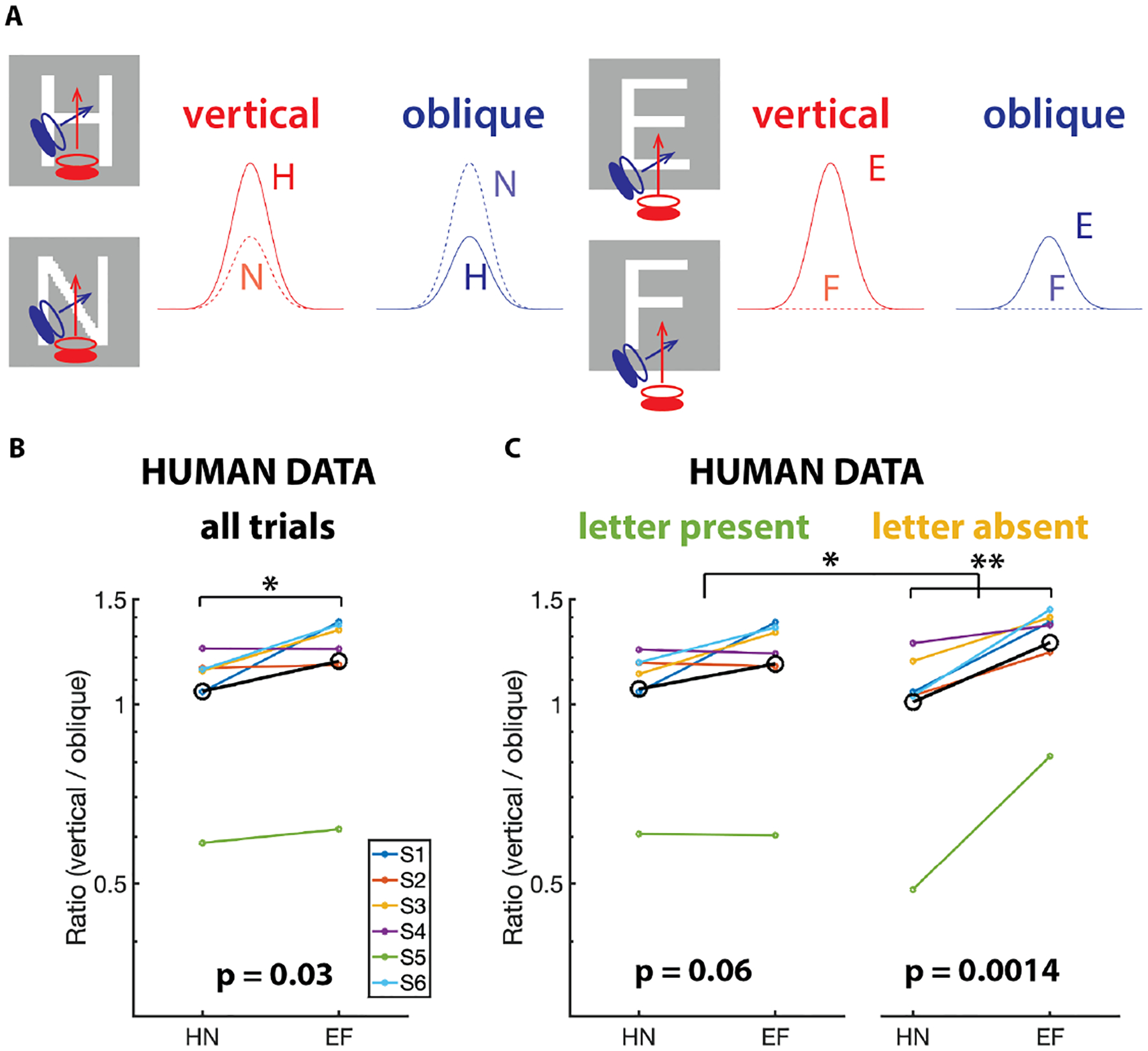
(A) Time course of the response of a model V1 simple cell during drifts. Eye motion was simulated as vertical (bottom to the top) or oblique (lower left to upper right). Schematics of the firing profiles are illustrated. Note that the two directions of drift yield signals that discriminate equally well between H and N (left). But to discriminate between E and F, vertical drift yields a stronger signal than oblique drift (right). (B) Comparison of measured vertical and oblique drift velocities. The ordinate is the ratio of the mean-squared velocity in the vertical direction to the mean-squared velocity orthogonal to the oblique stroke of the N estimated across all trials. p=0.03. (C) Same analysis as B, but separating the trials with letter-present and letter-absent. p=0.06 for letter-present, p=0.0014 for letter-absent, p=0.018 for comparison between letter-present and letter-absent conditions. One-tailed paired t-tests in (B) and (C). See also Figure S1.

In contrast, in the E vs. F discrimination, the only critical element is horizontal, and horizontally-oriented neurons will respond more strongly when moving along the vertical orientation. In this case, vertical drifts should elicit stronger cortical responses, facilitating discrimination, as illustrated in Figure 1A. We, therefore, would expect cognitive control to alter the distribution of drift orientations, favoring vertical over oblique motion when the subject engages in E vs. F discrimination.

Interestingly, a standard model of retinal ganglion cells (RGCs) leads to the same prediction. The reason is that motions that cross a bar orthogonally yields a shorter transit time than motions that cross a bar obliquely. This difference, coupled with the temporal properties of RGCs, generates a larger predicted response for motions orthogonal to the critical stimulus features than for oblique motions (see Figure S1D).

To test this prediction, we compared the amount of drift motion on the two axes relevant for this task, vertical and oblique. We computed the ratio of mean-squared drift velocities between the two axes, R = V_vertical/V_oblique, and then compared R_EF to R_HN. Figure 1B shows the average R_EF and R_HN across all subjects (in black) and for each individual. Supporting our hypothesis, on average across all trials types (i.e. with stimulus either present or absent), R_EF was indeed larger than R_HN (p < 0.05, one-tailed paired t-test), suggesting cognitive control of ocular drift.

Previous work has suggested that ocular drift can be influenced by the nature of the visual target^6,11. These influences may include components due solely to task knowledge (open-loop), and components that require a sensory response to the stimulus (closed-loop). By analyzing trials in which no stimulus was present – but in which the subject blueplanned an H vs. N or an E vs. F discrimination, we isolated components that are necessarily open-loop.

Figure 1C shows the results from this analysis. The variance ratio is estimated from just the letter-present (left) or just the letter-absent (right) trials. Both conditions show a trend towards more vertical drifts in the EF condition, but the difference is significantly more prominent in the letter-absent condition (p=0.0014 for letter-absent, p=0.06 for letter-present, p=0.018 for comparison between conditions, one-tailed paired t-test in all cases because our hypothesis specifies the direction of the change). Thus, we confirm that task knowledge influences ocular drift orientation, and that this influence is primarily via open-loop control.

Individual differences in drift modulation

Figure 1 shows that, on average, observers change their drift behavior according to the specific discrimination they engage in. Since drift characteristics are also known to vary considerably across individuals, the question emerges of how each subject tuned their idiosyncratic pattern of eye movements to the task. We therefore turned to a more comprehensive measure of drift statistics than the ratio of two directional velocities. In keeping with previous observations¹², drift velocity distributions were well approximated by two-dimensional Gaussians (Figure S2A). We, therefore, summarized these distributions by their covariances, visualized as covariance ellipses (Figure 2A). This displays the dominant drift orientation as the major axis of the covariance ellipse (indicated by the arrow’s orientation) and the degree of anisotropy as its deviation from circularity (indicated by the arrow’s length).

Figure 2: Individual drift velocity pattern depends on stimulus set.

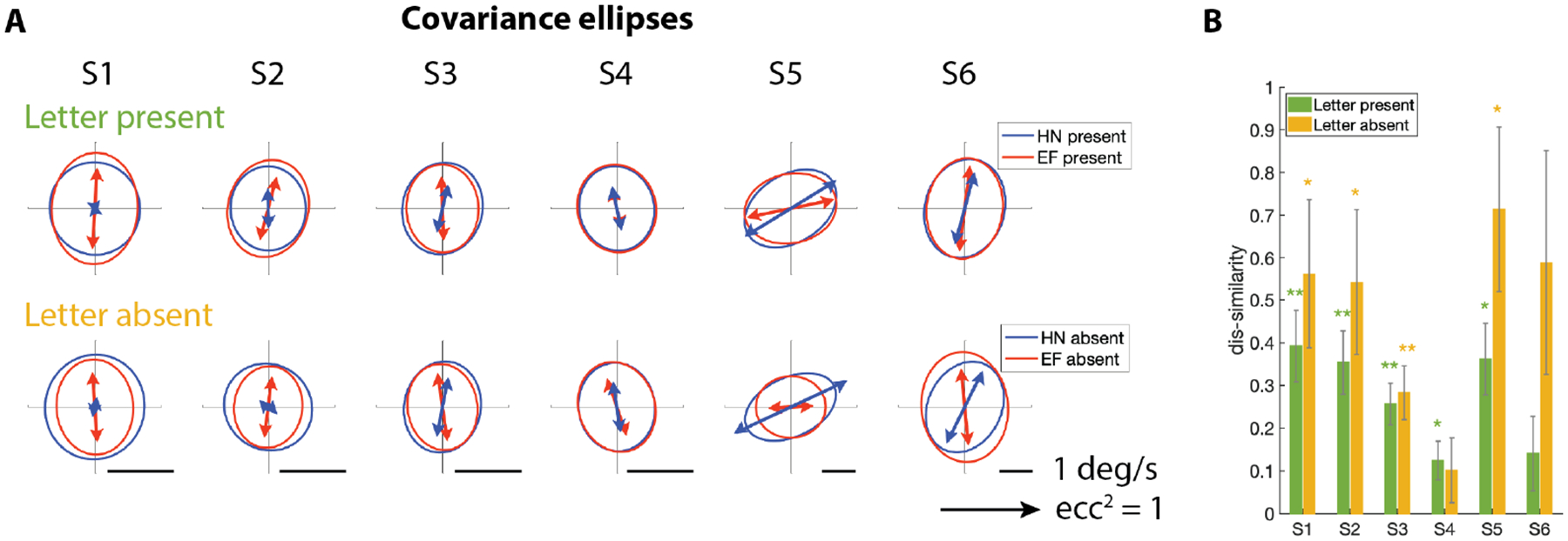
(A)Drift velocity covariance ellipses from HN trials(blue) and EF trials (red). Top: letter-present trials. bottom: letter-absent trials. Covariance ellipses cover 95% of the probability distribution of drift velocities; the arrow’s orientation is the major axis of the ellipse and its length is the anisotropy, measured as the square of the eccentricity. (B) Dis-similarity between HN and EF covariance ellipses in each subject. Green: letter-present trials. Orange: letter-absent trials (Error bars: 1 standard deviation. * p<0.05, ** p<0.01). See also Figure S2, S3, and S4.

This analysis showed that three observers (S1, S2, S3) exhibited a dominant orientation that was more nearly vertical in the EF trials, either in direction, magnitude, or both. S6 exhibited a similar trend in the letter-absent trials, although this change did not reach statistical significance. S4 showed very little change across trial types, whereas S5 exhibited a different behavior, namely a dominant oblique orientation in the HN trials and a horizontal orientation in the EF trials. We will show below that these seemingly disparate behaviors can all be explained by a common visuomotor strategy shared across subjects (see Figure 4).

Figure 4: A common control strategy despite individual differences in drift characteristics.

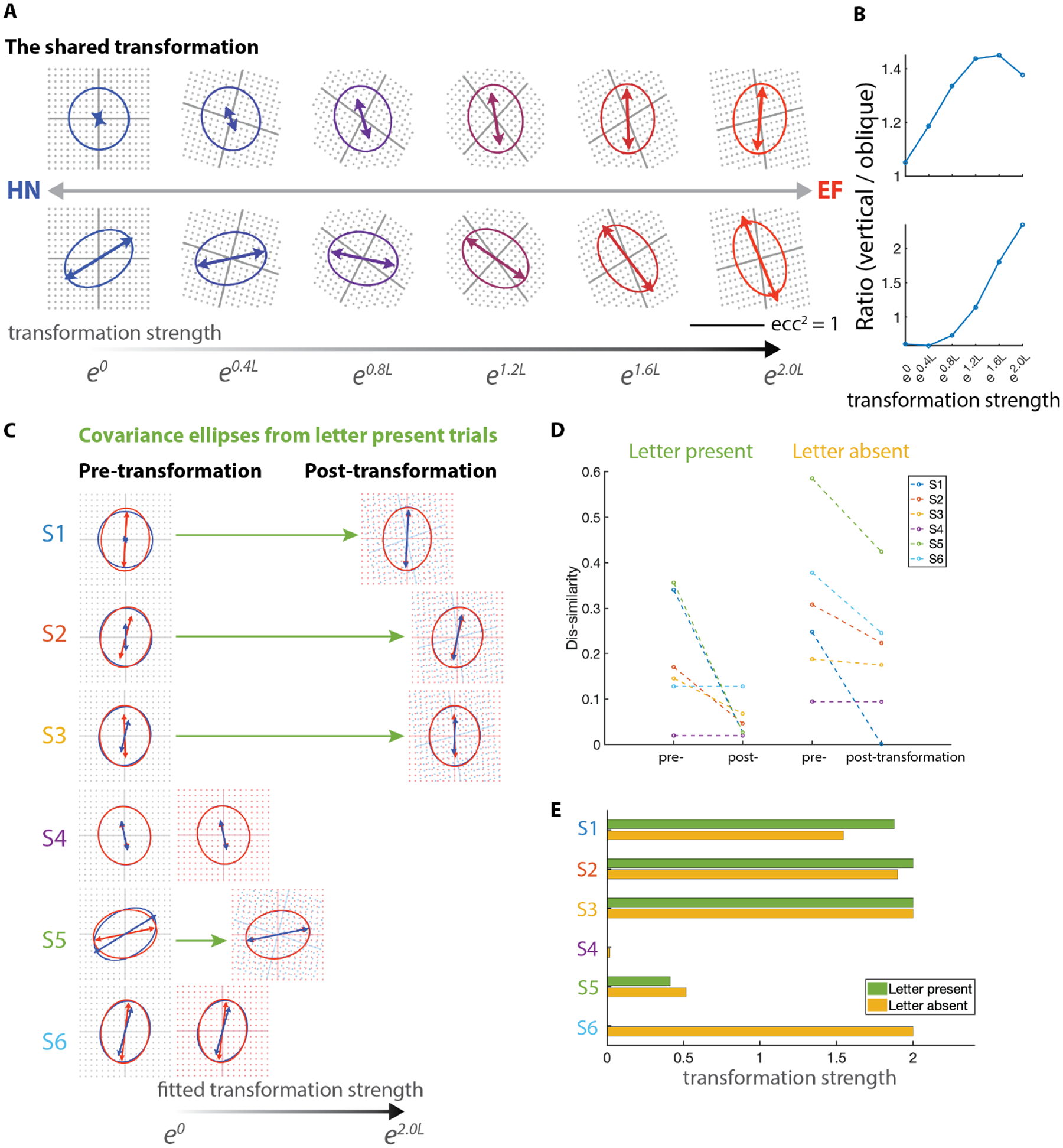
(A) Visualization of the shared transformation by applying graded amounts of the transformation to the HN ellipses from subject 1 (top row) and subject 5 (bottom row). Arrows indicate the dominant direction of the drift velocities, and their lengths indicate the degree of anisotropy. (B) The ratio of the mean-squared velocity in the vertical direction to the mean-squared velocity orthogonal to the oblique stroke of the N in each graded transformation in panel A. (C) HN (blue) and EF (red) covariance ellipses for each subject before and after applying varying amounts of the shared transformation. See Methods for details. (D) Dis-similarities of HN and EF covariance ellipses before and after applying the shared transformation. Left: target present trials. Right: target absent trials. (E) The amount of transformation applied in each subject.

To measure the overall influence of task on drift statistics in individual observers, we measured the dis-similarity between covariance matrices in the two conditions. This measure (standard for comparing 2 × 2 symmetric matrices, see Methods) considers differences in size, shape, and orientation, and weighs orientation more strongly with increasing eccentricity. Figure 2B shows the probability that this dis-similarity between HN and EF trials would have arisen by chance, given the observed trial-to-trial variability of ocular drift. Statistically significant differences (p < 0.05) were present in 5 out of the 6 subjects in the letter-present trials. Strikingly, statistically significant differences also occurred in the letter-absent trials (Figure 2) in 4 subjects. Thus, our results indicate that most subjects change their drifts based on prior knowledge of the discrimination to be made, and in most subjects, this difference is present in the letter-absent trials (open-loop) as well.

Conversely, by comparing drifts during the periods in the H trials and the N trials when the letter is present, or by making the parallel comparison in the EF blocks, we isolated components that are necessarily closed-loop. No subject showed a difference between FEM statistics in these comparisons.

We also found that there was no difference in drift trajectory curvature for HN vs. EF trials (Figure S2B) (two-tailed Wilcoxon signed rank test, p > 0.05 within each subject; two-tailed paired t-test across subjects, p > 0.05). Given our hypothesis, this was not surprising: while curvature increases in a high-acuity task⁶, it does not measure drift direction.

Drift velocity distribution changes are independent of microsaccades and block-to-block difference

Microsaccades can be influenced by cognitive factors^6,13,14, and indeed, we found that microsaccade landing points differed in HN vs. EF trials (see SI & Figure S3). However, this was not the basis of the differences in drift statistics: repeating our analysis, restricted to drifts that were at least 100 ms away from any other type of eye movement (Figure S4A–D), as well as excluding trials with any microsaccade, showed the same shift in drift statistics between HN and EF trials reported in Figure 2, for both letter-present and letter-absent trials. Thus, the cognitive influence on drift statistics is distinct from any cognitive influence on microsaccades.

Our findings were also not due to block-to-block differences in eye movements independent of the letter pair to be discriminated. To show this, we compared the difference between HN and EF consensus ellipses with that of surrogate data sets in which entire blocks were relabeled in a balanced randomized fashion. Statistical significance (p < 0.05) was present in 4 subjects in one or both of the two trial types (letter-present, letter-absent) (Figure S4E & F).

Decoding single-trial trajectories

The above results identify specific task-driven influences on ocular drifts during letter discrimination. Given that these influences occurred in most subjects, we wondered whether the resulting difference in velocity distributions suffices to identify the task (HN vs. EF) from a single trial eye trajectory. To focus on the shape difference of covariance ellipses, we normalized their size and computed their dis-similarities (Figure 3A & B). Subtle but significant shape differences of the normalized covariances were seen in HN vs. EF conditions for letter-present (4 subjects) and letter-absent (2 subjects) trials.

Figure 3: Decoding single trials via their drifts.

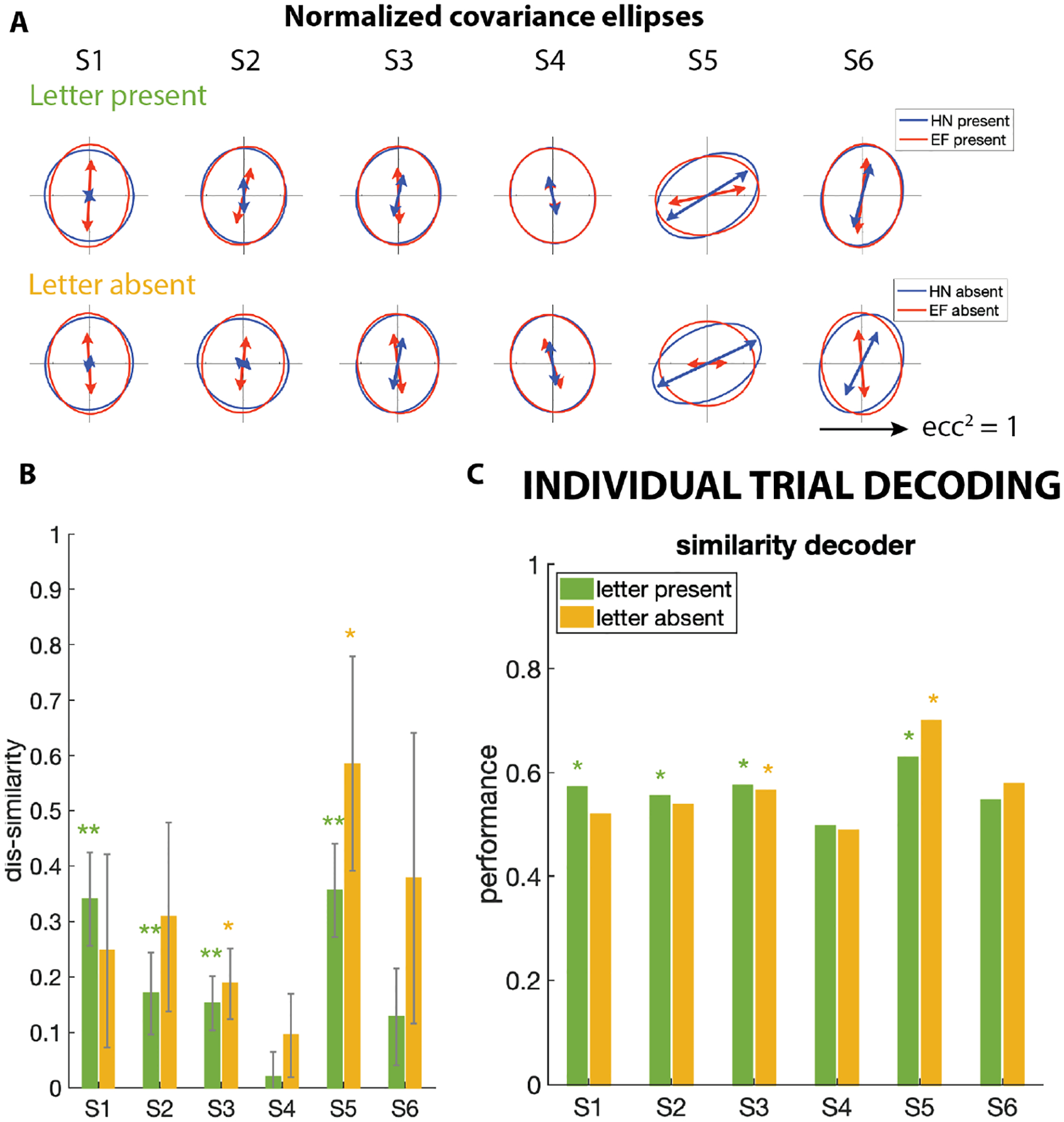
(A & B) Analysis of Figure 2 applied to covariance ellipses after normalizing to the same total area. In Panel A, the direction of the arrows indicate the dominant orientation of drift velocities, and their lengths indicate the degree of anisotropy. (C) Drifts from 300-ms periods of individual trials were decoded into task (HN vs. EF blocks) based on the similarity of the single trial covariance to the covariance estimated form all trials of each condition. The panel shows the performance of the similarity decoder across subjects; * indicates fraction correct higher than chance (p < 0.05) by binomial statistics.

We built a decoder that compared the velocity covariance measured in an individual trial to the normalized covariances estimated across all HN or EF trials (omitting the decoded trial). As described above, covariances were estimated from 300 ms of drifts during each trial and normalized. The decoder then assigned the held-out trial to the EF or HN block according to whether its covariance ellipse was more similar to the subject’s HN average, vs. the EF average. Figure 3C shows that this ”similarity decoder” identified the task (HN vs EF) from the drift trajectory at above chance levels whenever a subject showed a difference in drift covariances between HN and EF blocks, both in the letter-present trials or the letter-absent trials (Figure 3B). Very similar results were obtained by decoding the trials by maximum likelihood, i.e., by comparing the likelihood of a given trial’s trajectory, given the consensus ellipse for each trial type. Thus, in the subjects that exhibit cognitive drift modulations, it is possible to predict with better-than-chance accuracy the task that the subject prepares to tackle just by looking at the drift covariances.

A shared transformation across subjects

The task-dependent changes in drift statistics seen in Figure 2 vary across subjects, both in quality and magnitude. We hypothesized that there might be a single underlying transformation that accounts for all subjects’ changes in drift velocity distributions: for the vertical dominance in EF trials in some subjects, and the oblique dominance in HN trials in others, and for the changes in anisotropy of the velocity signals (Figure 3A & B). That is, we sought a single coordinate transformation, which, when applied with a subject-specific strength, would account for the change from HN to EF normalized covariance ellipses in all subjects. Formally, this corresponds (see Methods) to seeking a common coordinate transformation L and subject-specific strengths s_k, so that the coordinate transformations $e^{s_{k}L}$ account for the transformations between the HN and EF ellipses. This transformation L could produce a combination of rotation and stretching. The search for L was done by minimizing the dis-similarity between covariance ellipses after applying this transformation.

Figure 4A shows the inferred shared transformation of the velocity distribution by progresssively applying graded amounts of this transformation, using the HN ellipses of subjects S1 and S5 as a starting point. This shows that the shared transformation encompasses two behaviors: (1) If the covariances for the HN condition are close to isotropic (as for S1, top row of panel A), the full transformation leads to a covariance ellipse which has a dominant vertical orientation for the EF condition. (2) If the covariances are strongly anisotropic in the oblique orientation (as for S5, bottom row of panel A), the ellipse does not attain a vertical orientation and passes through a transitional stage with a nearly horizontal dominant orientation — accounting for this subject’s data in Figure 2A. Interestingly, irrespective of covariance patterns, application of this common transformation always increases the ratio of horizontal/oblique motion (Figure 4B). This holds even when graded amounts of the transformation yields an ellipse with a dominant horizontal direction, as in the transitional stages in the bottom row of Figure 4A.

Moreover, application of the shared transformation in varying degrees (Figure 4C) also accounts for the range of findings in all subjects who exhibited significantly different drift behaviors between in HN and EF blocks, including S5, in which the dominant direction in the EF condition is horizontal.

To understand whether top-down cognitive influences on eye drifts results in similar changes, we applied the same transformations to the corresponding letter-absent trials. Figure 4D shows the dis-similarity changes after applying the transformation, and Figure 4E shows the transformation strength applied. Interestingly, this shared transformation (along with the same subject-dependent strengths s_k) effectively decreased the dis-similarity in most subjects, as shown in Figure 4D. This implies that the task-dependent change is at least partially independent of visual stimulation. Thus, despite the large individual variability, there is a common open-loop strategy for controlling drift velocity distributions according to the letter pair to be discriminated.

DISCUSSION

FEMs are an essential part of the machinery that actively collects and process visual information during fixation. It is known that FEMs are modulated by the general characteristics of a visual task — for example, they slow in high-acuity tasks, and this maps higher spatial frequencies into the retina’s temporal sensitivity range⁶. Here we found a qualitatively different level of control: ocular drifts are influenced by the detailed characteristics of visual stimuli, and this influence can occur in an open-loop fashion based on specific task knowledge. When discriminating between two known-in-advance letters, subjects alter their drifts to emphasize orientations orthogonal to the distinguishing features of the letter pairs. Importantly, these effects were observed in most subjects even when no target was present, indicating the influence of task knowledge independent of visual information. In addition, this open-loop influence was comparable or even larger than the closed-loop effect (see Figure 2B & Figure 3B). Based on the modulation in individual trials, we showed that it is possible to identify the ongoing task, i.e., the letter pair being discriminated. Finally, we found that the drift velocity differences between the two kinds of letter-pair trials (HN, EF) could be accounted for by a shared transformation of drift velocity distributions, indicating a common strategy across subjects despite well-known idiosyncratic differences in drift characteristics.

The level of FEM cognitive control we discovered is highly specific and indicative of its possible purpose: increasing the luminance transients driven by the stimulus features that are task-relevant. Independently, the top-down control of microsaccades helps spatial selection within the foveal field, selecting the portion of the stimulus that is most relevant for the task. Together, both benefit visual perception by using cognitive strategies, knowledge, and experience to better acquire visual information.

It is worth noting that our findings indicate a commonality of drift control across subjects, despite the intersubject variability in FEMs during letter discrimination. Specifically, speed of drifts and speed change vary across subjects, and some subjects frequently make microsaccades, whereas others do so only rarely. These differences may in part reflect variation in subjects’ eye structure. For example, different densities of the cone mosaic¹⁵ could favor different magnitudes of drifts. Although it remains unclear what exactly determines the characteristics of each drift period, our data show a within-subject dependence of drift statistics based on the specific task and that the individual differences can be understood in terms of a shared transformation of the coordinates in which drifts are controlled.

Our findings concerning the influence of cognitive factors on FEMs need to be integrated into current understanding of neural mechanisms of eye movement control. Since amplitudes of microsaccades and saccades form a continuum^12,14,16,17, the obvious hypothesis is that cognitive influences over microsaccades and saccades travel along the same pathways. Several studies have probed the neural basis of how saccade and microsaccade generation depend on visual cues^18–20, but little is known about how microsaccade generation and drift generation interact. Additionally, since alterations of fixational eye movements are present in a range of ophthalmological²¹ and neurological disorders^22,23, characterization of FEMs and their control has the potential to be a clinical diagnostic tool.

Lastly, our findings raise the question of which brain structures are involved in open-loop control of drifts. Drift control is likely to involve the same cortical^18,19,24,25 and cerebellar^10,26 regions that are involved in control of fixation. But one cannot rule out direct cognitive control of brainstem circuitry. Critically, to account for our findings, the control pathway must provide task-specific directional information.

STAR METHODS

RESOURCE AVAILABILITY

Lead contact

Further information and requests for resources should be directed to and will be fulfilled by the lead contacts, Yen-Chu Lin (yel2005@alumni.weill.cornell.edu).

Materials availability

This study did not generate new unique reagents.

Data and code availability

Anonymized data created for the study are available in a persistent repository upon publication (Data Type: human eye movement tracing; Repository Name: Zenodo; DOI: https://doi.org/10.5281/zenodo.7647536). Any additional information required to reanalyze the data reported in this paper is available from the lead contact upon request.

EXPERIMENTAL MODEL AND SUBJECT DETAILS

Subjects

6 healthy subjects participated in the study (4 females and 2 males; average age: 27; age range: 22–31). Subjects were naive about the purpose of the study, were compensated for their participation, and provided informed consent. To qualify, subjects had to possess at least 20/20 acuity in the right eye (after correction if needed), as assessed by correct identification of at least 75% of the optotypes in the 20/20 line of a standard Snellen test. All procedures were approved by the Research Subjects Review Board at the University of Rochester and the Institutional Review Board of Weill Cornell Medical College.

METHOD DETAILS

Apparatus

Stimuli were displayed on an LCD monitor (Acer Predator XB272) at a refresh rate of 240 Hz and spatial resolution of 1920×1080 pixels and a background mean luminance of 18 cd/m². Subjects performed the task monocularly with their right eye; the left eye was patched. A dental-imprint bite bar and a headrest were used to minimize head movements. The movements of the right eye were measured by means of a custom digital Dual-Purkinje Image (dDPI) eye-tracker²⁷, a system with subarcminute resolution and internal noise of 0.07 arcsec^28,29. The eye position signals were sampled at 340 Hz.

Task & stimuli

Healthy human subjects performed two-alternative letter discrimination tasks, with stimuli presented on an LCD monitor in a dark room. Blocks of trials (each consisting of 50–100) were of two types, one in which they discriminated H vs. N and one in which they discriminated E vs. F. We refer to these as HN and EF trials, respectively. Blocks were presented in interleaved order and subjects were informed of the letter pair to be discriminated at the start of each block. In all blocks, each letter was presented in 40% of the trials, and 20% of trials contained only noise. Letters were in Helvetica font and subtended approximately 1.5°. They were presented in positive contrast and superimposed on a 2° square patch of 1/f noise (f from 1 to 16 cycles per degree), with a root-mean-squared contrast of 0.195 (see Figure S1C for examples).

To keep task diffculty comparable across subjects and over time, we manipulated the contrast of the letter so that performance was 75% in preliminary trials on each day. The same contrast was used for the HN and EF trials.

Subjects initiated the trial with a button-press, which triggered the appearance of fixation point, a small white square. Once the subject maintained fixation of the center within 0.5 deg for 600 ms, the trial began with the presentation of stimulus at the center of the display. Contrast (letter and noise) was ramped up linearly for 1 sec, held at a plateau for 500 ms, and then off (see Figure S1B). Subjects had to respond within 5 seconds after the stimulus reached plateau by a button-press.

QUANTIFICATION AND STATISTICAL ANALYSIS

Data analysis

Data analysis began with a pre-processing stage in which trials were parsed into periods of microsaccades and drifts, along with rejection of trials with poor tracking, artifacts, blinks, or large saccades. Following this, we carried out several quantitative analyses of drifts and microsaccades and their relationship to the task, visual stimuli, and performance.

The preprocessing stage uses standard techniques reported in previous publications^6,13, and is summarized here. The raw position signal on each channel (horizontal and vertical) was first filtered and differentiated by means of a Savitzky-Golay filter with cutoff frequency at approximately 30 Hz, and an effective smoothing window of 20 ms. The eye trajectory was then parsed into periods of large saccades, microsaccades, and fixational drifts. As in previous publications using the DPI eye-tracking method, movements with maximum speed higher than 3°/sec and amplitude larger than 0.5°were classified as saccades. The amplitude was defined as the distance between the locations at which eye velocity became greater (onset) and lesser (offset) than 2°per sec. Microsaccades were defined as saccades with amplitudes smaller than 30 arcmin. The segments between saccades or microsaccades were labeled as periods of fixational drifts. Trials with large saccades and with eye movements that moved fixation beyond the bounds of the stimulus were discarded. See Table S1 for the summary of the numbers of trials given conditions in all six subjects.

To select trials for FEM analysis, we excluded trials containing blinks or artifacts from head movements or the eye tracker. All occurrences of microsaccades during the entire stimulus presentation (including the contrast ramp) were analyzed. For analysis of drift, we further excluded trials with drift velocities over 5 deg/s, so that the analysis would not be contaminated by small undetected microsaccades. For each valid trial, we then extracted the first available 300 ms period that did not include times within 50 ms of a saccade or microsaccade, beginning with the time at which stimulus contrast was maximal. The exclusion of times near saccades or microsaccades was to control for possible artifacts in the estimation of the instantaneous in velocity of ocular drift resulting from these rapid movements. All such 300 ms periods of drifts from valid trials were then pooled together for further drift analysis.

Ocular drift analysis.

To compare two drift velocity distributions, we first estimated drift velocity covariance ellipses from all trials, and then quantified the dis-similarity between conditions as described below. The best-estimate ellipses illustrated (e.g., in Figure2A & Figure 3A) were 95% probability contours.

Statistical significance of the difference in covariances was determined by comparing the observed difference in covariances to an empirical null distribution. The empirical null distribution was created from 1000 surrogate datasets, each generated by randomly relabeling trials as HN or EF, regardless of the actual stimulus. We then computed the dis-similarity between the covariance ellipses derived these surrogate datasets, and determined the fraction of the surrogate dis-similarity values that exceeded the dis-similarity value computed from the actual data.

To include the effects of block-to-block variations in eye movements (Figure S4E & F), surrogate datasets were computed by balanced block relabeling of half of the blocks (6–11 blocks in each condition, 1000 draws).

Comparison of shapes of 2-D distributions.

To quantify the difference in the shape of two-dimensional distributions between conditions, e.g., between drift velocity distributions in HN and EF trials (Figures2B & 3B), we proceeded as follows. We first parameterized the shape of each distribution by fitting it with a two-dimensional Gaussian. Since the shape of a two-dimensional Gaussian is determined by its covariance matrix, we quantified the difference in shape by a standard distance on the set of two-dimensional symmetric positive definite real matrices³⁰. For covariance matrices C₁ and C₂, this distance is defined by

$$d_0\left(C_1,C_2\right)=\sqrt{{\mathit{\text{log}}}^2\left({\lambda }_1\right)+{\mathit{\text{log}}}^2\left({\lambda }_2\right)}$$ (1)

where λ_i are the two eigenvalues of $C_1^{-1}{C}_2$. Note that the distance is zero only if the λ_i are both 1, i.e., if C₁ = C₂.

The distance is appropriate for comparing shape since it takes into the account size differences, eccentricity differences, and orientation differences, and considers orientation more strongly when the shape becomes more eccentric. In addition, the distance remains unchanged if both covariance matrices are multiplied by the same scale factor or rotated by the same amount.

To compare 2-D distributions after normalization by size (Figure3B), the covariance matrices of the two distributions were each divided by the square root of their determinants (i.e., the areas of the corresponding ellipses) before computing the above distance.

Curvature (k) of drift trajectories on individual trials was determined from the first and second derivatives of the eye position (x, y) at each time, using code kindly provided by J. Intoy and used in Intoy et al.⁶.

$$k=\frac{\left|x^{\prime }{y}^{\prime \prime }-y^{\prime }{x}^{\prime \prime }\right|}{{\left(x^{\prime 2}+y^{\prime 2}\right)}^{3/2}}$$ (2)

Microsaccade analysis.

To study the properties of microsaccades, we compared the scatter of landing position distributions between HN and EF trials. All the microsaccades made during stimulus display were analyzed. To characterize landing position distributions (FigureS3), we found the minimumarea ellipse covering 95% of the landing points^31,32. To compare landing point locations, we computed the Euclidean distance between the centers of these ellipses. Statistical significance of these measures was determined by comparison to an empirical null distribution computed by trial shuffing (100 draws).

Decoding

We tested two decoding strategies to identify single-trial trajectories based on the task-driven influences, a similarity decoder and a maximum likelihood decoder. For both decoders, the HN and EF consensus covariance ellipses were estimated by pooled drift segments but omitting the trials to be decoded.

For the similarity decoder, the single-trial covariance was estimated based on 300 ms of drift segment. The decoder then assigned the trials based on the least distance (eq.1) between the normalized single-trial covariance and the normalized consensus HN or EF covariances.

The maximum likelihood decoder identified single-trial trajectories based on the estimated log-likelihood of the single-trial drift velocities $(\overrightarrow{v})$ emerging from the distribution of either the HN or EF velocity distribution. This in turn was determined by considering each of the measured velocities in the trial to be decoded as independent draws from a Gaussian with the consensus covariance matrix (C_HN or C_EF ). For example, the probability that a velocity ${\overrightarrow{v}}_j$ is drawn from the HN distribution is given by

$$P_{HN}\left({\overrightarrow{v}}_j\right)=\frac{1}{2\pi \sqrt{\mathit{\text{det}}\left(C_{HN}\right)}}{e}^{\frac{-{\overrightarrow{v}}_j^T{C}_{HN}^{-1}{\overrightarrow{v}}_j}{2}},$$ (3)

so the log likelihood for a velocity sequence $\overrightarrow{v}=\left\{{\overrightarrow{v}}_1,\dots ,{\overrightarrow{v}}_N\right\}$ is given by

$$\frac{1}{N}\text{log\hspace{0.17em}}p\left(\overrightarrow{v}\mid C_{HN}\right)=-\text{log\hspace{0.17em}}(2\pi )-\frac{1}{2}\text{log}\left(\mathit{\text{det}}\left(C_{HN}\right)\right)-\frac{1}{2N}\sum _j\left({\overrightarrow{v}}_j^T{C}_{HN}^{-1}{\overrightarrow{v}}_j\right).$$ (4)

Identifying a shared coordinate transformation underlying changes in covariance ellipses

As described above, the strategy for comparing the drift velocity distributions in HN vs. EF conditions is to compare their normalized covariances C_HN and C_EF, which was done by computing $C_{HN}^{-1}{C}_{EF}$ and then determining the distance between this matrix and the identity matrix. To test the possibility that the different covariance changes observed in each subject resulted from the same basic coordinate transformation, but with each subject applying it in different amounts, we proceeded as follows. First, we note that a coordinate transformation Z, where Z is a potential combination of rotation, stretching, and scaling, results in a transformation of the covariance C_HN to Z^T C_HNZ. To formalize the idea of varying amounts of the same coordinate transformation, we define the infinitesimal of the transformation Z as a transformation L for which Z = e^L. In this way, the set of coordinate transformations e^sL can be viewed as the transformations that result from applying Z with variable strength: the original Z = e^sL for s = 1, and Z² = e^sL for s = 2, the result of applying the transformation Z twice. More generally, e^sL is the result of applying the transformation Z s times, and e^sL is meaningful even when s is not an integer.

With this in mind, we sought a coordinate transformation L common to all subjects, along with values of the strengths s_k specific to each subject k, that minimized the total of the squares of the distance between the subject’s observed covariances C_HN,k and the subject’s observed covariances C_EF,k, after transformation of C_HN,k by $e^{s_{k}L}$. To treat the two conditions equally, we implemented this by applying half of the transformation to the HN ellipse ${\left(e^{\frac{s_k}{2}L}\right)}^T{C}_{HN,k}\left(e^{\frac{s_k}{2}L}\right)$ and half of the inverse transformation to the EF ellipse ${\left(e^{\frac{-s_k}{2}L}\right)}^T{C}_{EF,k}\left(e^{\frac{-s_k}{2}L}\right)$, and then carried out a nonlinear optimization that minimized the sum of squares of the distances defined in eq.1 between them (the “residual dis-similarity”). The results of this calculation are shown in Figure 4C & D. Since the overall size of s and L trade off, we added the requirement that tr(L^T L) = 1.

A challenge in evaluating the statistical evidence for a shared transformation is the lack of an a priori model for the repertoire of drift patterns that a subject can make. We therefore resorted to an exceedingly conservative hypothesis: that each subject’s repertoire of covariances for each condition is limited to the anisotropy we observed, and that the ability of a subject to shift their covariance was limited to the observed changes between tasks. Based on this hypothesis, we generated surrogate data in which covariance patterns were randomly associated with each task. We then used these surrogate datasets to assess the likelihood that a shared transformation would reduce the dis-similarity by the amount we observed in the actual data (Figure 4D). Specifically, surrogate datasets were generated by random application of three manipulations within each subject: swapping the covariance ellipses between the two conditions, rotation of the two ellipses by the same amount, and mirroring the ellipses across the y-axis. For each surrogate dataset, we determined the shared transformation and then computed the reduction in dissimilarity that it accounted for. Remarkably, even with this exceedingly conservative approach, the observed consistency across subjects (i.e., the reduction in dis-similarity due to the shared transformation determined from the actual data) was found in only 14% of the surrogate data – strongly suggesting the presence of a shared transformation, given the overly stringent nature of the test.

A standard model of RGCs

In Figure S1D, we simulate the neuronal activity elicited in the early visual pathway by the retinal stimuli using previous published spatiotemporal receptive field models of RGCs^33–37. These models specify both spatial and temporal filtering properties at the LGN level that transform the retinal input into a firing rate. The receptive field model (K) contains the center and surround, each with its own separable spatial and temporal components³⁶.

$$K(x,y,\tau )=F_c(x,y)G_c(\tau )-F_s(x,y)G_s(\tau )$$ (5)

The center and surround spatial profiles F_c or F_s are described by a 2-D circular Gaussian distribution:

$$F(x,y)=C{e}^{\frac{-\left(x^2+y^2\right)}{2\pi {\sigma }^2}}$$ (6)

The parameters (C & σ) were taken from experimental recordings in macaque monkeys and typically differ for center and surround³⁵. Following the work of Victor in 1987³⁷ , we use a series of low-pass and high-pass stages with transfer function to describe the temporal filtering properties.

$$\tilde{G}(\omega )=A{e}^{-i\omega D}\left(1-\frac{H_s}{1+i\omega {\tau }_s}\right){\left(\frac{1}{1+i\omega {\tau }_L}\right)}^{N_L}$$ (7)

The parameters (A, D, H_s, τ_s, τ_L, N_L) were taken from experimental recordings in macaque monkeys and typically differ for center and surround^33,34.See Lin (2022) for more details of the model³⁸.

References

- 1.Yarbus AL (1967). Eye movements and vision (Springer; ). [Google Scholar]
- 2.Henderson JM (2017). Gaze Control as Prediction. Trends Cogn Sci 21, 15–23. URL https://www.ncbi.nlm.nih.gov/pubmed/27931846. [DOI] [PubMed] [Google Scholar]
- 3.Kowler E, Anderson E, Dosher B, and Blaser E (1995). The roleof attention in the programming of saccades. Vision Res 35, 1897–916. URL https://www.ncbi.nlm.nih.gov/pubmed/7660596. [DOI] [PubMed] [Google Scholar]
- 4.McPeek RM, Maljkovic V, and Nakayama K (1999). Saccades require focal attention and are facilitated by a short-term memory system. Vision Res 39, 1555–66. URL https://www.ncbi.nlm.nih.gov/pubmed/10343821. [DOI] [PubMed] [Google Scholar]
- 5.Rucci M and Victor JD (2015). The unsteady eye: an informationprocessing stage, not a bug. Trends Neurosci 38, 195–206. URL https://www.ncbi.nlm.nih.gov/pubmed/25698649. [DOI] [PMC free article] [PubMed] [Google Scholar]
- 6.Intoy J and Rucci M (2020). Finely tuned eye movements enhance visual acuity. Nat Commun 11, 795. URL https://www.ncbi.nlm.nih.gov/pubmed/32034165. [DOI] [PMC free article] [PubMed] [Google Scholar]
- 7.Aytekin M, Victor JD, and Rucci M (2014). The visual input to theretina during natural head-free fixation. J Neurosci 34, 12701–15. URL https://www.ncbi.nlm.nih.gov/pubmed/25232108. [DOI] [PMC free article] [PubMed] [Google Scholar]
- 8.Poletti M, Aytekin M, and Rucci M (2015). Head-Eye Coordination at a Microscopic Scale. Curr Biol 25, 3253–9. URL https://www.ncbi.nlm.nih.gov/pubmed/26687623. [DOI] [PMC free article] [PubMed] [Google Scholar]
- 9.Leigh RJ and Zee DS (2015). The Neurology of Eye Movements (Oxford University Press; ). URL https://oxfordmedicine.com/view/10.1093/med/9780199969289.001.0001/med-97801999 [Google Scholar]
- 10.Kheradmand A and Zee DS (2011). Cerebellum and ocular motor control. Front Neurol 2, 53. URL https://www.ncbi.nlm.nih.gov/pubmed/21909334. [DOI] [PMC free article] [PubMed] [Google Scholar]
- 11.Gruber LZ and Ahissar E (2020). Closed loop motor-sensory dynamics in human vision. PLoS One 15, e0240660. URL https://www.ncbi.nlm.nih.gov/pubmed/33057398. [DOI] [PMC free article] [PubMed] [Google Scholar]
- 12.Cherici C, Kuang X, Poletti M, and Rucci M (2012). Precision ofsustained fixation in trained and untrained observers. J Vis 12. URL https://www.ncbi.nlm.nih.gov/pubmed/22728680. [DOI] [PMC free article] [PubMed] [Google Scholar]
- 13.Shelchkova N and Poletti M (2020). Modulations of foveal vision associated with microsaccade preparation. Proc Natl Acad Sci U S A 117, 11178–11183. URL https://www.ncbi.nlm.nih.gov/pubmed/32358186. [DOI] [PMC free article] [PubMed] [Google Scholar]
- 14.Ko HK, Poletti M, and Rucci M (2010). Microsaccades preciselyrelocate gaze in a high visual acuity task. Nat Neurosci 13, 1549–53. URL https://www.ncbi.nlm.nih.gov/pubmed/21037583. [DOI] [PMC free article] [PubMed] [Google Scholar]
- 15.Putnam NM, Hofer HJ, Doble N, Chen L, Carroll J, and Williams DR (2005). The locus of fixation and the foveal cone mosaic. J Vis 5, 632–9. URL https://www.ncbi.nlm.nih.gov/pubmed/16231998. [DOI] [PubMed] [Google Scholar]
- 16.Rucci M and Poletti M (2015). Control and Functions of Fixational Eye Movements. Annu Rev Vis Sci 1, 499–518. URL https://www.ncbi.nlm.nih.gov/pubmed/27795997. [DOI] [PMC free article] [PubMed] [Google Scholar]
- 17.Martinez-Conde S, Otero-Millan J, and Macknik SL (2013). The impact of microsaccades on vision: towards a unified theory of saccadic function. Nat Rev Neurosci 14, 83–96. URL https://www.ncbi.nlm.nih.gov/pubmed/23329159. [DOI] [PubMed] [Google Scholar]
- 18.Edelman JA and Goldberg ME (2001). Dependence of saccade-related activity in the primate superior colliculus on visual target presence. J Neurophysiol 86, 676–91. URL https://www.ncbi.nlm.nih.gov/pubmed/11495942. [DOI] [PubMed] [Google Scholar]
- 19.Hafed ZM, Goffart L, and Krauzlis RJ (2009). A neural mechanism for microsaccade generation in the primate superior colliculus. Science 323, 940–3. URL https://www.ncbi.nlm.nih.gov/pubmed/19213919. [DOI] [PMC free article] [PubMed] [Google Scholar]
- 20.Hafed ZM, Yoshida M, Tian X, Buonocore A, and Malevich T (2021). Dissociable Cortical and Subcortical Mechanisms for Mediating the Influences of Visual Cues on Microsaccadic Eye Movements. Front Neural Circuits 15, 638429. URL https://www.ncbi.nlm.nih.gov/pubmed/33776656. [DOI] [PMC free article] [PubMed] [Google Scholar]
- 21.Kumar G and Chung ST (2014). Characteristics of fixational eyemovements in people with macular disease. Invest Ophthalmol Vis Sci 55, 5125–33. URL https://www.ncbi.nlm.nih.gov/pubmed/25074769. [DOI] [PMC free article] [PubMed] [Google Scholar]
- 22.Pinnock RA, McGivern RC, Forbes R, and Gibson JM (2010). An exploration of ocular fixation in Parkinson’s disease, multiple system atrophy and progressive supranuclear palsy. J Neurol 257, 533–9. URL https://www.ncbi.nlm.nih.gov/pubmed/19847469. [DOI] [PubMed] [Google Scholar]
- 23.Kapoula Z, Yang Q, Otero-Millan J, Xiao S, Macknik SL, Lang A, Verny M, and Martinez-Conde S (2014). Distinctive features of microsaccades in Alzheimer’s disease and in mild cognitive impairment. Age (Dordr) 36, 535–43. URL https://www.ncbi.nlm.nih.gov/pubmed/24037325. [DOI] [PMC free article] [PubMed] [Google Scholar]
- 24.Segraves MA (1992). Activity of monkey frontal eye field neurons projecting to oculomotor regions of the pons. J Neurophysiol 68, 1967–85. URL https://www.ncbi.nlm.nih.gov/pubmed/1491252. [DOI] [PubMed] [Google Scholar]
- 25.Stanton GB, Goldberg ME, and Bruce CJ (1988). Frontal eye field efferents in the macaque monkey: II. Topography of terminal fields in midbrain and pons. J Comp Neurol 271, 493–506. URL https://www.ncbi.nlm.nih.gov/pubmed/2454971. [DOI] [PubMed] [Google Scholar]
- 26.Krauzlis RJ, Goffart L, and Hafed ZM (2017). Neuronal control of fixation and fixational eye movements. Philos Trans R Soc Lond B Biol Sci 372. URL https://www.ncbi.nlm.nih.gov/pubmed/28242738. [DOI] [PMC free article] [PubMed] [Google Scholar]
- 27.Wu RJ, Clark AM, Cox M, Intoy J, Jolly P, Zhao Z, and Rucci M (2022). High-resolution eye-tracking via digital imaging of Purkinje reflections. BioRxiv. [DOI] [PMC free article] [PubMed] [Google Scholar]
- 28.Rucci M, Wu RJ, and Zhao Z (2021).
- 29.Intoy J, Mostofi N, and Rucci M (2021). Fast and nonuniform dynamics of perisaccadic vision in the central fovea. Proc Natl Acad Sci U S A 118. URL https://www.ncbi.nlm.nih.gov/pubmed/34497123. [DOI] [PMC free article] [PubMed] [Google Scholar]
- 30.Lim LH, Sepulchre R, and Ye K (2019). Geometric Distance BetweenPositive Definite Matrices of Different Dimensions. IEEE Transactions on Information Theory 65, 5401–05. [Google Scholar]
- 31.Rousseeuw RJ and Driessen KV (1999). A Fast Algorithm for the Minimum Covariance Determinant Estimator. Technometrics 41, 212–223. URL https://www.tandfonline.com/doi/abs/10.1080/00401706.1999.10485670. [Google Scholar]
- 32.Hubert M, Rousseeuw PJ, and Van Aelst S (2008). High-BreakdownRobust Multivariate Methods. Statistical Science 23, 92–119, 28. URL 10.1214/088342307000000087. [DOI] [Google Scholar]
- 33.Benardete EA and Kaplan E (1997). The receptive field of the primateP retinal ganglion cell, I: Linear dynamics. Vis Neurosci 14, 169–85. URL https://www.ncbi.nlm.nih.gov/pubmed/9057278. [DOI] [PubMed] [Google Scholar]
- 34.Benardete EA and Kaplan E (1999). The dynamics of primate M retinal ganglion cells. Vis Neurosci 16, 355–68. URL https://www.ncbi.nlm.nih.gov/pubmed/10367969. [DOI] [PubMed] [Google Scholar]
- 35.Croner LJ and Kaplan E (1995). Receptive fields of P and M ganglion cells across the primate retina. Vision Res 35, 7–24. URL https://www.ncbi.nlm.nih.gov/pubmed/7839612. [DOI] [PubMed] [Google Scholar]
- 36.Rucci M, Edelman GM, and Wray J (2000). Modeling LGN responses during free-viewing: a possible role of microscopic eye movements in the refinement of cortical orientation selectivity. J Neurosci 20, 4708–20. URL https://www.ncbi.nlm.nih.gov/pubmed/10844040. [DOI] [PMC free article] [PubMed] [Google Scholar]
- 37.Victor JD (1987). The dynamics of the cat retinal X cell centre. J Physiol 386, 219–46. URL https://www.ncbi.nlm.nih.gov/pubmed/3681707. [DOI] [PMC free article] [PubMed] [Google Scholar]
- 38.Lin YC (2022). Psycophysical and physiological study of active visionvia fixational eye movements. Ph.D. thesis, Cornell University. [Google Scholar]
Associated Data
This section collects any data citations, data availability statements, or supplementary materials included in this article.
Supplementary Materials
Data Availability Statement