Bézier Curve Method to Compute Various Meniscus Shapes

Abstract

This paper is an extension of our earlier paper in which it was shown that the meniscus shape in a cylindrical capillary could be computed by solving the Young–Laplace equation via optimization of a Bézier curve. This work extends the previous work by demonstrating that the method is applicable to predict the meniscus shape not only in a cylindrical capillary but also in other cases, such as at a tilted plate, between two plates, and for a sessile drop. Numerous works have attempted previously to solve the Young–Laplace equation, and their results all agree with this paper’s validating its method. All the preceding approaches, however, used special techniques to solve the differential equation, while the Bézier curve method proposed in this work is more simple, which allows it to maintain greater computational simplicity. Moreover, the Bézier curve method can be applied to solve many other different differential equations in the same way as shown in this work. The effect of the Bézier curve degree on the precision of prediction was also thoroughly investigated. It was found that the 4th degree Bézier curve was required to predict the meniscus shape precisely in a cylindrical capillary, against a tilted plate, and between two plates, while the 5th degree was required for the shape of the sessile drop.

1. Introduction

The calculation of the meniscus shape is actively researched because of its importance in surface and interfacial science. For the meniscus in a cylindrical capillary, when R, the radius of the capillary, is significantly smaller than the capillary length, = 2.713 × 10^–3 m for water, where σ, ρ, and g are the surface tension of water, density of water, and gravity constant, respectively, the effect of gravity on the shape is negligible, so the meniscus can be accurately approximated with a spherical surface. There, the equation Δp = 2σ cos θ/R can be used, where θ is the contact angle, and R is the radius of the capillary. However, when R is significantly larger than the capillary length, gravitational force is more impactful, flattening the meniscus in the center and making the spherical approximation inaccurate. Thus, providing a more accurate description of the shape of the meniscus under the effect of gravity is an area of active research. (It should be noted that the capillary length is defined as a point, where the gravity and surface forces are in equilibrium. It is often used for the meniscus calculation of different shapes, as shown in the following examples).

For example, Eslami and Elliot evaluated the depth of capillary menisci by considering the three-phase contact line as the initial point for the integration of the differential equations they developed.¹ Bullard and Garboczi minimized the free energy to calculate the meniscus shape in a cylindrical capillary, as well as the capillary rise between two closely placed parallel planar surfaces.² Lobanov calculated the shape and volume of the meniscus at the upper horizontal plane of a specimen, at the lower horizontal plane of a specimen, and at the surface of a cylindrical specimen.³ Biery and Oblak modified the Young–Laplace equation to a differential equation in which the two radii of curvature are shown differently. Using this equation, they numerically calculated the meniscus shape and validated the calculation by experiments.⁴ Soligno et al. proposed a numerical method to calculate the meniscus shape between vertical and inclined walls and curved surfaces by minimizing the thermodynamic potential of the system.⁵ Henriksson and Erikson defined the capillary rise in a cylindrical capillary rigorously.⁶ Ward and Sasges introduced explicit expressions for the chemical potentials in the Laplace equation and found that the condition on the chemical potentials could be used to determine the pressure profile within the system.⁷ Malijevský and Parry dealt with the meniscus of a liquid confined between an open capillary slit, showing that there are two types of competing meniscus shapes, corresponding to corner filling and meniscus depinning transitions.⁸ Recent publications also reveal the continuing interest in this subject. For example, Behroozi discussed the applications of the Young–Laplace equation in hydrostatics, such as the differential pressure within soap bubbles and liquid droplets, the rise and fall of liquids in capillaries, and the depth of liquid spills.⁹ Liu et al. presented an analytical solution in the planer model and the numerical solution to the axisymmetric model on the meniscus shape and compared the results against Jurin’s law (the maximum height of the capillary rise is inversely proportional to the capillary diameter), modified Jurin’s law, and Surface Evolver simulation.¹⁰ Lv and Shi extended the analytical expression of the droplet shape on a flat surface to the shape of the droplet on an inclined surface.¹¹ Tang and Cheng systematically studied the meniscus on the outside of a small circular cylinder immersed vertically in a liquid bath in a cylindrical container using the Young–Laplace equation.¹² Eißman et al. presented three-dimensional calculations of the meniscus of a magnetic fluid placed around a current-carrying vertical and cylindrical wire.¹³ Liu et al. computed the meniscus shape around a fiber vertically piercing into the water surface to mimic the strider leg on the water surface.¹⁴ Liu et al. also computed the meniscus of a pendant droplet.¹⁵

In all the abovementioned methods, a point-by-point balance is established between surface tension and gravitational force, which leads to the Young–Laplace differential equation. These equations are solved either analytically or numerically under a certain boundary condition. There is another method, in which the meniscus shape is obtained by minimizing the total energy, including the potential energy term and surface energy term, of the system. The method called “Surface Evolver” was proposed by Brakke to study the shapes that are governed by surface tension. Starting from an initial surface, the program evolves it toward the minimum energy state by interacting with the user. The advantage of this method is that it can draw the shape of very complex geometries.¹⁶

Concerning the meniscus between two vertical plates with different contact angles, Laplace mentioned that the meniscus is lifted at the surface of the lower contact angle and dropped at the surface of the higher contact angle, with an inflection point on the meniscus. O’Brien, Craig, and Peyton measured the capillary rise between two vertical plates, one made of glass (CA of 14°) and the other coated with PTFE (CA of 110°), and fitted their experimental data by the equation

1

where h is the capillary rise, θ₁ and θ₂ are the contact angles against the glass plate and coated glass plate, respectively, and w is the distance between the two plates.¹⁷

Concerning the meniscus at a vertical plate partially immersed in liquid, Neumann derived the equation

2

where h′ is the meniscus height.¹⁸

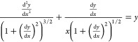
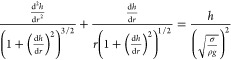
Concerning the shape of a sessile droplet on a horizontal surface, Bashford and Adams derived the differential equation.¹⁹ In a dimensionless form, it is written as

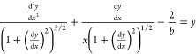3

where x and y are x = r/l and y = h/l (see Figure 1), respectively, and b is equal to .

Figure 1.

Schematic representation of the shape of a sessile drop on a horizontal plate.

Dang et al.,²⁰ and Srinivasan et al.²¹ also used the differential eq 3 to calculate the shape of a sessile drop.

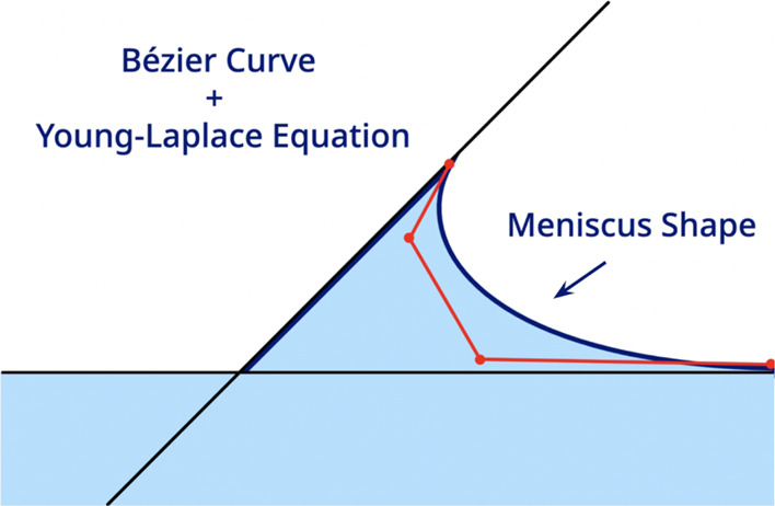
Note that all the preceding approaches used certain mathematical techniques to solve the differential equation, while the Bézier curve method proposed in this paper is simpler. Moreover, the Bézier curve method can also be applied to solve different differential equations and cases in the same way.

The Bézier curve is a parametric function, consisting of one polynomial function for each dimension. Therefore, like polynomials, Bézier curves can be of any degree and express complicated shapes as the degree increases. An nth-degree Bézier curve is defined by n + 1 points, called P₀, P₁, ... P_n. The curve begins at P₀, goes in the direction of each of the intermittent points, and then ends at P_n. The Bézier curve method can approximate the solution of any differential equation by changing the parameters of the Bézier curve to minimize the difference between the two sides of the differential equation. According to Venkataraman, the Bézier curve is advantageous when solving differential equations for four main reasons: its approximations are accurate, its formulation is simple, the differential equations can be handled in their original forms, and standard optimization techniques can be applied.²²

Indeed, a number of papers have been published to show that the differential equations can be solved by the Bézier curve method accurately and efficiently. Some of the examples are as follows:

Ghomanjani and Hadi Farahi used the Bézier method to solve delay differential equations approximately.²³ Some examples have also been given to demonstrate the efficiency of the method. Ghomanjani and Khorram presented a method to solve a quadratic Riccati differential equation by using Bézier curves and gave some examples to demonstrate the simplicity and efficiency of the proposed method.²⁴ Ghomanjani and Shateyi solved one-dimensional Bratu’s problem by the Bézier method, and the efficiency and accuracy of the method were demonstrated by some numerical examples.²⁵ Sweitzer and Kumar solved approximately systems of ordinary and partial differential equations by using solvers such as the ones Gurobi developed in Operations Research. The entire functions were represented by Bézier curves or surfaces with appropriate control points.²⁶ Venkataraman solved approximately the linear partial differential equation by using the Bézier method as an extension of the solution of the ordinary differential equation. The method was applied for the solution of several engineering problems, such as the Poison equation, one-dimensional heat equation, and the slender two dimensional cantilever beam.²² Manikandan and Kamanat solved three dimensional Navier Stokes equations near the rotating disk by using the Bézier curve method, and the results were compared with the numerical solution given by the conventional boundary value problem solver.²⁷ Narooei and Taheri used the Bézier method to analyze the equal channel angular extrusion process of a rectangular cross section. Predicted values agreed very well with the experimental ones for two dies with different outer curved corner.²⁸ Zheng et al. solved differential equations numerically by the least squares method using the control points of a Bézier curve. The convergence of the method was further analyzed.²⁹

Thus, the objective of this work is to calculate 1) the meniscus shape in a cylindrical capillary, 2) the meniscus between two vertical plates of different contact angles, 3) the meniscus at a vertical plate partially immersed in a liquid, and 4) the shape of a sessile drop on a horizontal surface, under gravity, by applying the Bézier curve method to solve the Young–Laplace differential equation. The precision of the solution is further evaluated and related to the degree of the Bézier curve.

2. Method

2.1. Differential Equations and the Bézier Curve Method

The differential equation applicable for each case of the set objectives of this work has been found in the literature, as summarized in the second column of Table 1 together with its boundary conditions. The details of these differential equations and the boundary conditions are explained later.

Table 1. Summary of Differential Equations and Boundary Conditions.

meniscus	differential equation	boundary conditions	reference and comments
in a cylindrical capillary		dy/dx = 0 at x = 0, dy/dx = cot θ at x = xn	(4, 22)
between two vertical plates with different contact angles		dy/dx = −cot θla at x = 0, dy/dx = cot θra at x = xn	(2)
at a slanted plate		dy/dx = −cot(φ + θ)b at x = 0, dy/dx = 0, at x = xn which is very large
as a droplet on a horizontal surface	c	dy/dx = 0, at x = 0, dy/dx = −tan θd, at x = xn	(18−21)

^aθ_l and θ_r are the contact angles at the left and right plates, respectively.

^bφ is the tilt angle and θ is the contact angle at the plate.

^c.

^dθ is contact angle at the horizontal plate.

The Bézier curve method to solve the differential equations is demonstrated for the cubic Bézier (the 3rd Bézier) curve as an example, as follows.

The position of a point in the cubic Bézier curve at some time t is

4

From this equation, the x and y values at some time t are

5

6

Therefore, x′, y′, x″, and y″ over t can be calculated easily by differentiating eqs 5 or 6 once or twice over t. Since 5 and 6 are polynomials in terms of t, this can be done symbolically easily using a computer algebra system, the one used here being SageMath, and the result will be another polynomial. (Note that dy/dx = y′/x′ and d²y/dx² = (x′y″ – y″x′)/(x′)²).

Accordingly, the left- and right-hand sides of the differential equation can be calculated for a given set of the Bézier parameters (x₀, x₁, x₂, x₃, y₀, y₁, y₂, and y₃) over t, and the difference is called D(t).

The differential equation is solved by optimizing the Bézier parameters (x₀, x₁, x₂, x₃, y₀, y₁, y₂, and y₃) to make D(t) as close to 0 for as many values of t as possible. For this purpose, quantity loss is defined as

7

Then, the parameters are chosen to minimize loss.

Note that D(t) is evaluated at 20 points of t, including t = 0 and 1, with an equal interval in between. Among the parameters to be optimized, some are fixed: for example, x₀ and x₃, the beginning and the end of the Bézier curve, respectively, are the beginning and end of the meniscus. In addition, the boundary conditions may fix some other parameters.

Sage expands and calculates the loss symbolically. Then, it is minimized with the Sage minimize() function, which uses Scipy’s simplex algorithm. This function requires some initial values. In most cases, all x’s are set equal to and all y’s are set to 1. However, these were sometimes changed, especially when the loss was larger than expected. The result with the smallest loss was always accepted.

The same method can be applied to the 4th degree Bézier curve to find polynomial forms for x, y, x′, y′, x″, and y″ in terms of t since the position of a point in the 4th degree Bézier at time t is

8

Similarly, the position of a point in the 5th degree Bézier is

9

In general, the position of a point in the nth degree Bézier is written as

10

It should be noted that the pinning force is ignored in this approach.³⁰

2.2. Meniscus in a Cylindrical Capillary

Figure 2 schematically depicts the meniscus formed in a cylindrical capillary.

Figure 2.

Schematic representation of the meniscus in a cylindrical capillary.

By considering a force balance on a small section of the meniscus surface, the differential eq 11 is derived based on the Young–Laplace.⁴ The same equation can be derived by minimizing the Helmholtz energy of the system.³¹

11

where r and h are the radial distance from the center of the cylinder and the longitudinal distance from a reference point, respectively (see Figure 2). Note that the first and second terms of eq 11 correspond to the reciprocal of the principal radii of curvature involved in the Young–Laplace equation.

Let l = the capillary length. Then, eq 11 can be rewritten in a dimensionless form as

12

where x = r/l and y = h/l.

Equation 12 is solved with the boundary conditions

13

14

where x_n = R/l (R is the radius of the cylindrical capillary), and θ is the contact angle.

In a Bézier curve, dy/dx at t = 0 is the same as the slope between P₀ and P₁, and dy/dx at t = 1 is the same as the slope between P_n–1 and P_n. Therefore, we can remove two unknowns by setting

15

16

Note that these conditions solve for half the meniscus. To see the full meniscus, one must combine this image with its mirror over the y axis.

2.3. Meniscus between Two Vertical Plates with Different Contact Angles

The menisci formed between two vertical plates with contact angles of θ_l and θ_r are shown schematically in Figure 3.

Figure 3.

Schematics of the meniscus between two plates with different contact angles.

Bullard and Garboczi made the prediction of the meniscus shape for such a system² by a differential equation

17

where x = d/l and y = h/l.

In differential eq 17, the second term of eq 12 is removed since one of the principal radius curvatures is infinity, and its effect on the capillary force can be ignored.

The boundary conditions are

18

19

where x_n = D/l (D is the half of the distance between the plates.)

These boundary conditions can be manipulated to remove two unknowns

20

21

Note that, by the same reasoning as the single plate, the plates can be slanted as well. However, the plates should not cross; in that case, the water cannot flow freely from the water level to the meniscus, so Bullard and Garbozci’s differential equation no longer applies.

2.4. Meniscus at a Single Plate

Figure 4 shows schematically the meniscus at a plate immersed partially in water with a tilted angle of φ.

Figure 4.

Schematic representation of the meniscus on a plate immersed partially in water with a tilted angle of φ.

As shown in Table 1, the differential equation to be used is the same as that of the meniscus between two plates with different contact angles.

The boundary conditions, however, are different.

22

and

23

The x_n value at which the boundary condition 23 is satisfied will be investigated in the results section.

These boundary conditions can be manipulated to remove two unknowns

24

25

2.5. Shape of the Sessile Drop

As shown in Table 1, the differential equation is

26

where x = r/l, y = h/l, and .

The boundary conditions are

27

28

where x_n = R/l.

These boundary conditions can be manipulated to remove two unknowns

29

30

3. Results and Discussion

3.1. Effect of the Order of the Degree of Bézier Curve on the Accuracy of the Calculation

In order to investigate the effect of the degree of the Bézier curve on the accuracy of the calculation, the meniscus between two vertical plates with different contact angles is used as an example.

In Figure 5, the red and blue lines represent, respectively, the left- and right-hand sides (LHS and RHS) of the differential eq 17 versus t. Note that the lines were drawn for the optimized Bézier parameters for each degree of the Bézier curve. The figure loss is also given. When the red and blue lines overlap, or come as close to each other as possible, at all values of t, the loss becomes near zero, and the accuracy increases for the solution of the differential equation.

Figure 5.

Left-hand side, (red) and right-hand side, y (blue) graphed over t from 0 to 1, corresponding to optimized Bézier parameters. (a) uses the cubic Bézier; (b–d) use the 4th degree Bézier.

Figure 5a,b shows the results obtained by the cubic (3rd degree) and 4th degree Bézier curves, respectively, when θ_l = 45°, θ_r = 14°, and x_n = 10. The 4th order provides much higher accuracy with a loss of 0.053 than the 3rd order with a loss of 0.209. x_n decreases progressively from 10 in Figure 5b to 3 in Figure 5c and further 1 in Figure 5d, which is accompanied by a decrease in loss from 0.053 to 0.009 and further to 0.001. As a result, both the red and blue lines overlap almost completely for x_n = 1. This means that the accuracy of the computation increases as the distance between the plates decreases.

3.2. Meniscus in a Cylindrical Capillary

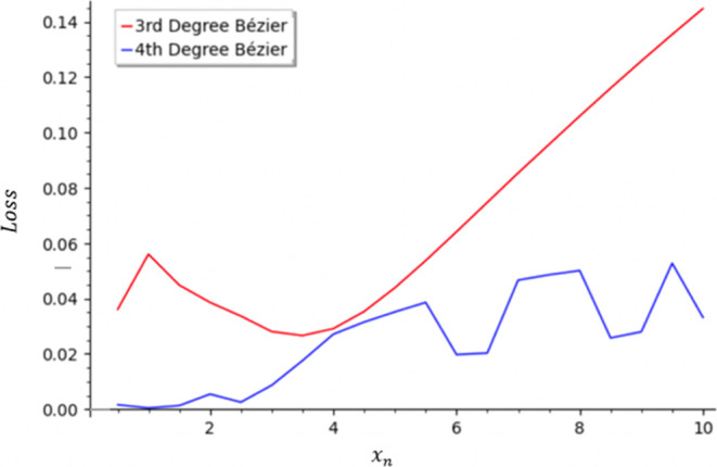
Figure 6 depicts the different loss values as x_n changes from the 3rd degree Bézier (red) to 4th degree Bézier (blue), when θ is fixed at 45°. For the 3rd degree Bézier, loss increases linearly as x_n increases, with an average of 0.002 for every 1 increase of x_n. For the 4th degree Bézier, loss is nearly equal to zero at x_n = 1 and then increases to 0.002 in a region of 2–4, before decreasing to 0.0008 again at x_n = 5. Losses do not increase substantially thereafter.

Figure 6.

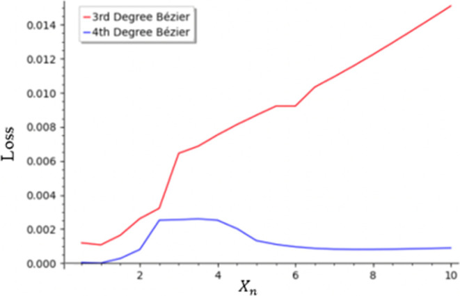
Minimum loss for different x_n when θ is fixed at 45° (red, 3rd degree; blue, 4th degree Bézier).

Thus, the 3rd Bézier curve method is unable to give an accurate answer for large x_n, particularly when a wide flat region appears due to the effect of gravitational force. An additional point in the Bézier curve of the 4th degree improves accuracy in this region.

Figure 7 depicts the minimum loss for different θs as θ ranges from 10 to 170°. The graphs are of such different scales that they are placed next to each other. The 3rd degree Bézier [(a) red] has much higher loss when the angle is very large or small but has a smaller loss in the middle. The 4th degree Bézier [(b) blue], on the other hand, has no apparent correlation, and the loss is 2 orders of magnitude lower than the 3rd degree.

Figure 7.

Minimum loss for different θs when x_n is fixed at 1 ((a) (red) 3rd degree, (b) (blue) 4th degree).

Thus, the 4th degree Bézier always provides better accuracy than the 3rd degree, especially when x_n is large or the contact angle is either very small or very large. Therefore, the 4th degree Bézier will be used hereafter for the meniscus in a cylindrical capillary.

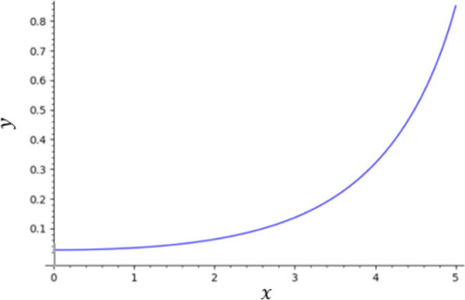
Figure 8 shows the effect of x_n on the meniscus height (see Figure 2), when θ is fixed at 45°.

Figure 8.

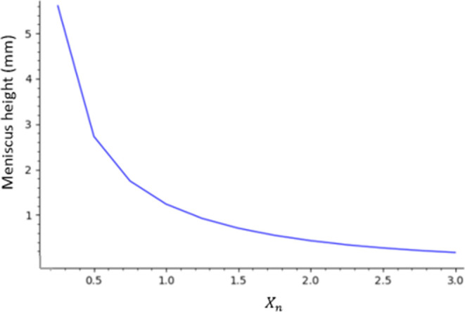
Meniscus height for different x_n when θ is fixed at 45° (meniscus height is measured to the bottom of the meniscus (y at x = 0 or r = 0 in Figure 2)).

The meniscus height decreases as x_n increases. This is because the effect of the surface force decreases as the cylindrical radius increases from x_n = 0.3 (R = 0.814 mm) to x_n = 3.0 (R = 8.14 mm), resulting in the decrease of the meniscus height from 5.6 to 0.2 mm. It is well known that water in a capillary rises more as the capillary size decreases.

These results obtained by the Bézier curve method were further compared against the data provided by Eslami and Elliot’s numerical calculation based on the differential equation that they had derived, which was essentially the same as eq 11.¹Figure 9 shows that these two methods generally agree on the meniscus depth, while θ goes from 25 to 75°, and R is fixed to 10 mm (x_n = 3.686). The Bézier model has more of a linear decrease, though, while Eslami and Eliott’s model curves upward slightly in the middle.

Figure 9.

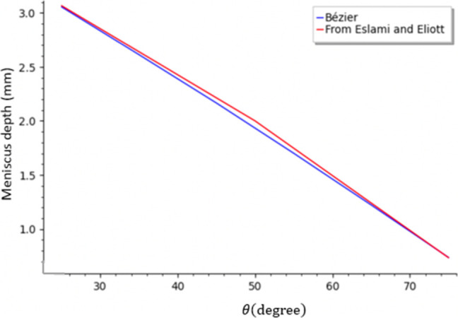
Comparison of meniscus depth calculated by the Bézier curve method with the data presented by Eslami and Eliott in Figure 11 of ref (1) (for different θs at R = 10 mm).

Figure 10 shows the meniscus depths provided by both methods when R goes from 5 to 40 mm (x_n from 1.843 to 14.74), and θ is fixed to 25°. In this case, both methods agree when R is smaller than 20 mm or larger than 70 mm, but the Bézier curve method predicts slightly lower values when R is between 20 and 70 mm.

Figure 10.

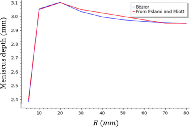
Comparison of meniscus depth calculated by the Bézier curve method with the data presented by Eslami and Eliott in Figure 11 of ref (1) (for different Rs at θ = 25°).

The Bézier curve method decreases more rapidly after the maximum at around 20 mm. Still, the difference is very small and is likely caused by difficulties in reading Eslami and Eliott’s data. It is interesting to note that the maximum of the meniscus depth could be reproduced by the 4th degree Bézier, unlike the 3rd degree Bézier that could not reproduce the maximum.³²

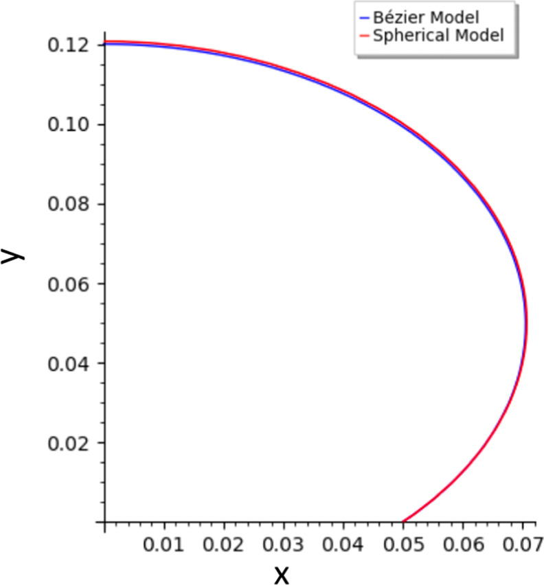
Figure 11 compares the calculated meniscus shape with a spherical model for a small capillary with x_n = 0.2. As mentioned earlier, the meniscus is part of a spherical surface when the capillary radius is smaller than the capillary length l. In the figure, only one curve is visible because the two curves are exactly overlapping. When the capillary radius is small, the meniscus shape can be accurately approximated by a sphere, so the spherical model is accurate. Therefore, if the Bézier model is so accurate in this already solved case, it is likely also accurate when the width is larger.

Figure 11.

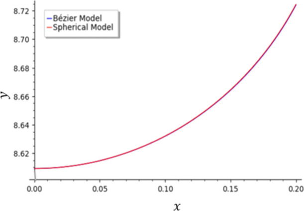
4th degree Bézier model (blue) and spherical model (red) of the meniscus when θ = 30° and x_n = 0.2.

Figure 12 displays an example of a meniscus drawn by the 4th Bézier curve method for x_n = 5 > 1. Note that the radius of the capillary (R = 13.565 mm) is five times as large as the capillary length, and the effect of gravity can no longer be ignored. Now the flat region appears in the center of the meniscus; this is due to the effect of gravity working in the center of the capillary.

Figure 12.

Meniscus of a cylindrical capillary with θ = 45° and x_n = 5, calculated by the 4th degree Bézier model (loss was 0.0013).

3.3. Meniscus between Two Plates with Different Contact Angles

Figure 13 shows the optimized loss for different x_n, while θ_l and θ_r are fixed. For the 3rd degree Bézier model, the loss increases linearly as x_n increases. Similar to the cylindrical capillary, this is likely because the 3rd degree Bézier is unable to calculate the height at the long flat region in the middle of the meniscus, while also calculating the edges poorly. The 4th degree Bézier also increases as x_n becomes larger, but much more slowly; for example, losses are 0.13 and 0.028, for the 3rd and 4th degree Bézier, respectively, at x_n = 9. At x_n = 10, the difference is even larger. When x_n is above 10, the two plates are far enough apart that the meniscus height is basically 0 in the middle. Therefore, it can be solved separately using the one-plate case twice, which is more accurate. Since the 4th degree Bézier model is always more accurate, it will be used hereafter.

Figure 13.

Minimum loss of 3rd and 4th degree Bézier curves for a two plate system as x_n changes, while θ_l and θ_r are fixed at 45 and 14°, respectively.

Figure 14 shows the loss as θ_l and θ_r change, while x_n is fixed at 1. The loss always stays below 0.0023. There is no apparent correlation between the contact angles and the loss in this case.

Figure 14.

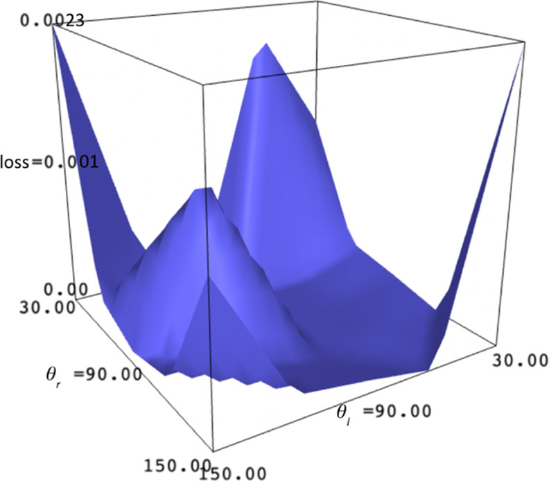
Loss as θ_l and θ_r are changed among 30, 60, 90, 120, and 150°, and x_n is fixed at 1 (this uses the calculations from the 4th degree Bézier model.).

The meniscus was calculated by the Bézier method for D = 2.5 mm, θ_l = 14 and θ_r = 45°, and the results are compared with the data of Bullard and Garboczi (given in Figure 4 of their paper²) in Figure 15.

Figure 15.

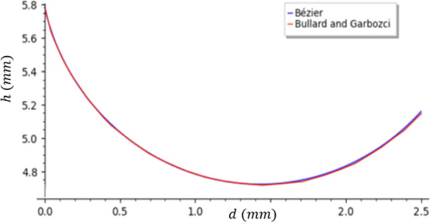
Comparison of the meniscus calculated by the Bézier method, and the data given in Figure 4 of Bullard and Garbozci² (D = 2.5 mm and θ_l and θ_r are 14 and 45°, respectively).

In the figure, the data from the two different sources almost completely overlap, with the Bézier method’s result being slightly higher on the right end.

3.4. Meniscus at a Single Plate

First, the meniscus shape was calculated when x_n was 100 for various φ + θ values. It was noticed that the y value was essentially 0 when x reached 5 in all cases, so the value of x_n at which the meniscus ends was set to 5. y is zero at x > 5.

From eqs 17, 22, and 24, it is obvious that the solution is unique to a given value of φ + θ. It is interesting to note that there are two mathematically valid solutions for a given value of φ + θ, when φ + θ > 90°, depending on the initial guess, and both solutions are physically meaningful. Those two cases correspond to the surfaces being either hydrophilic (θ < 90°) or hydrophobic (θ > 90°) (see Figure 16a,b).

Figure 16.

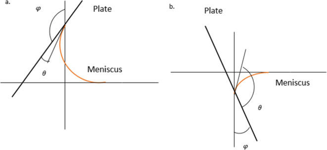
Meniscus between a plate and horizontal water surface formed when a tilted plate is partially immersed in water ((a) hydrophilic surface and (b) hydrophobic surface).

Figure 17 shows an example for φ + θ = 135°. These two results were generated from different initial values. In Figure 17a, the meniscus shape starts by going left, while in Figure 17b, the meniscus shape starts by going right. However, φ + θ = 135° for both. Both results could exist in the real world. Figure 17a could happen if the plate is slanted rightward and hydrophilic, and Figure 17b could happen if the plate is hydrophobic.

Figure 17.

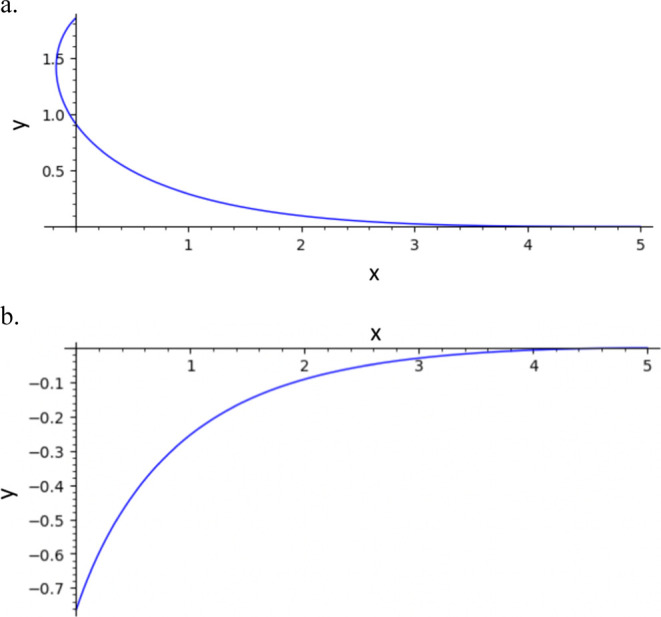
Two valid possible menisci for φ + θ = 135° (calculated using the 4th degree Bézier curve. (a) used initial values of x₁ = −5/4, x₂ = 5/2, x₃ = 15/4, y₀ = 1, and y₃ = 1, while (b) used initial values of x₁ = 5/4, x₂ = 5/2, x₃ = 15/4,y₀ = 1, and y₃ = 1).

The initial values can be determined deliberately to choose which results the computer gives. If x₁ is initially negative, then the meniscus shape will start by going left, but if x₁ is initially positive, the meniscus shape will start by going right. The Bézier parameters obtained at convergence were (0, 1.8467727149640079), (−0.5154921523027827, 1.3312805626612252), (0.010350793933075336, 0.01807437762745126), (1.5624322460612419, 0), and (5, 0) for Figure 17a and (0, −0.7647056505944001), (0.5443274009164648, −0.2203782496779353), (1.509651498000658, −0.10860846237353626), (2.1652509650623104, 0), and (5, 0) for Figure 17b.

Figure 18 displays the loss for different contact angles for the 3rd and 4th degree Bézier curves when the surface is hydrophilic. Both the 3rd and 4th degree Bézier show the same minimum loss of 0.0027 at θ = 75°, but the loss of the 3rd degree Bézier increases quickly as θ decreases.

Figure 18.

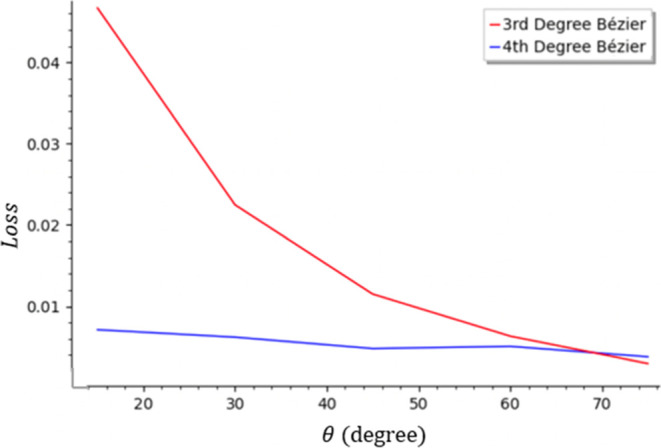
Loss value for the optimized Bézier parameters with 3rd and 4th degree Bézier curves as θ changes and φ remains constant at 0.

Newman, based on the rigorous solution of the Young–Laplace equation, derived eq 2 for the meniscus height when φ = 0, shown as h′ in Figure 19.¹⁸

Figure 19.

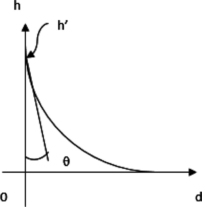
Schematic representation of the meniscus formed between a plate and horizontal water surface when the plate is immersed vertically in water.

After rearranging

31

Figure 20 shows h′/l versus θ calculated by the Bézier method and Neumann’s equation. The fit is almost exact; only one line is visible because they are exactly over each other. The agreement further validates the solutions by the Bézier method.

Figure 20.

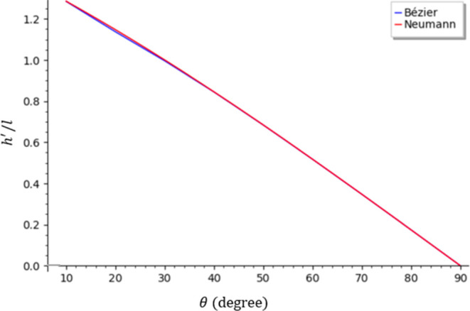
Comparison of h′/l versus θ obtained by the Bézier method and Neumann’s equation (changed from 10 to 90°).

3.5. Sessile Drop

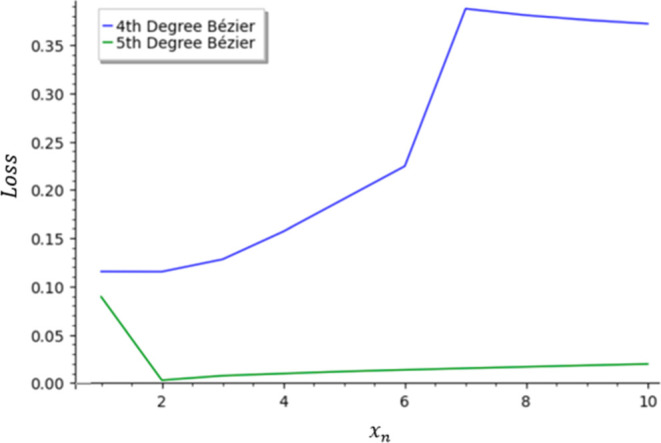
Figure 21 compares the minimum losses obtained by using the 3rd, 4^th, and 5th degree Bézier for different θs when x_n is fixed at 1. The 3rd degree Bézier increases exponentially as θ increases and is highly inaccurate in the large value range of θ. The 4th degree Bézier is very accurate in the beginning, with a loss of 0.0058 at θ = 30°, before increasing substantially at θ = 45° and staying at a maximum value of roughly around 0.1 afterward. The 5th degree Bézier starts significantly lower than even the 4th degree, with a loss of around 0.00005 from 15 to 60° and then increases to 0.0015 at 75°, before finally increasing to be similar to but slightly less than the 4th degree Bézier when θ is obtuse.

Figure 21.

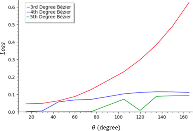
Comparison of 3rd, 4th, and 5th degree Bézier curves (for different θs and x_n = 1).

Figure 22 displays the minimum loss for the 4th and 5th degree Béziers as x_n is changed, while θ is kept constant at 135°. The 3rd degree Bézier is not considered since its loss is too high. The 4th degree Bézier increases greatly as x_n increases, because it does not have enough parameters to model the flat top and the curved side. The loss flattens out after x_n = 7 at a high loss of above 0.35. For the 5th degree Bézier, on the other hand, the minimum loss is the highest when x_n is 1, but it decreases at x_n = 2 and then increases very slowly. Therefore, the 5th degree Bézier needs to be used especially for the calculation of the shape of the drop on a horizontal surface.

Figure 22.

Comparison of 4th and 5th degree Bézier curves (for θ = 135° and different x_ns).

When the size of the drop is very small, it should be a perfect sphere since gravity does not have a very large impact. Figure 23 compares the Bézier model with the spherical model when θ is 135° and x_n is 0.05. At the bottom, they agree completely, but at the top of the meniscus, the Bézier model is slightly lower. This makes sense because the Bézier model takes gravity into account, while the spherical one does not. In general, however, they agree very well, so the Bézier predictions for the cases that cannot be approximated by a sphere are likely accurate as well.

Figure 23.

Comparison between the 5th degree Bézier model prediction and spherical model prediction for y versus x (for θ = 135° and x_n = 0.05).

Figure 24 compares the result of the Bézier curve with Dang et al.’s work (Figure 5 of their work¹⁸). Both largely agree, but the Bézier curve is slightly taller and skinnier.

Figure 24.

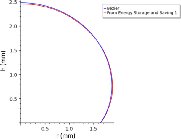
Comparison of the height versus distance from the center of the droplet between the Bézier curve and Dang et al.’s work for (for θ = 125° and R = 1.65 mm).

Figure 25 shows some examples of calculated shapes of sessile droplets with large sizes, that is, (a) with a radius of 27.13 mm and (b) with 13.57 mm, which are 10 times and 5 times larger than the capillary length, respectively. It should be noted that the droplet becomes flat in the central region because of the effect of gravity. Interestingly, when the contact angle is as large as 135°, the radius of the side of the droplet becomes larger than at the bottom.

Figure 25.

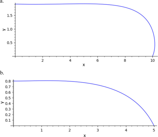
Some examples of the sessile droplet shape calculated using the 5th degree Bézier curve method ((a) θ = 135° and x_n = 10 and (b) θ = 45° and x_n = 5).

Notice that the volume of the sessile drop could be calculated based on the width using this method, so the width and shape of the sessile drop could be found based on the volume as well.

The experimentally measurable contact angle (CA) for a rough surface is an apparent CA, which may differ from the ideal CA for a smooth, solid surface. Especially for a rough surface with air-filled grooves, Cassie and Baxter proposed the following equation

32

where θ_Y and θ_CB are the CA (°) of a droplet resting on a smooth surface and the CA on a composite surface of solid and air, respectively. f_s is the fraction of the solid surface which is in contact with the liquid phase.³³ According to the equation, θ_CB increases from θ_Y to 180° as f_s decreases from 1 to zero. This principle is often used to develop a superhydrophobic surface.

Hereafter, an attempt is made to compute the water droplet shape on a surface with an air-filled hole at the droplet center to examine if the presence of such a hole indeed increases the CA, following the steps;

• 1)A meniscus shape on a smooth solid surface is computed by the Bézier curve method for a given dimensionless radius x and a CA (Figure 26a).
• 2)An arc is drawn above the air-filled hole. This arc is a part of a circle since the contact angle between water and air is 180°. The height of the circle is made equal to that of the meniscus drawn in step 1). Then, the (x, y) coordinates of the lower edge of the arc as well as the tangent (dy/dx) can be obtained (Figure 26b)).
• 3)The meniscus shape from the edge of the arc is computed by the Bézier curve method, using (x, y) and (dy/dx) obtained in step 2, until it arrives at the solid plate surface (Figure 26c).

Figure 26.

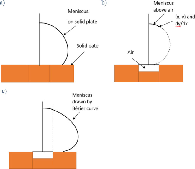
Schematic representation of the steps to calculate the meniscus shape on a plate with an air-filled hole ((a) meniscus on a smooth solid plate, (b) meniscus on the air, and (c) meniscus drawn by the Bézier curve method).

For an example computation,

• 1)We start from a dimensionless radius x = 0.608 and a CA θ_Y = 130° to compute the meniscus shape on a smooth solid plane. The meniscus height becomes 1.08.
• 2)The (x, y) coordinate and the slope (dy/dx) at the edge of the arc are calculated to be (0.286, 1.00) and −0.623, respectively.
• 3)The Bézier curve is drawn. It ends at a point (0.602, 0).

The meniscus so computed is illustrated in Figure 27. The shape of the droplet is more sagging in the lower part of the meniscus when there is a hole in the plate. This shape was observed experimentally for a water droplet formed on the surface with a hole.³⁴ As a result, the CA increased from 130° on the smooth, solid plate to 140° on the plate with a hole, showing that the presence of an air-filled hole makes the plate more hydrophobic. According to eq 32, θ_CB is 136°.

Figure 27.

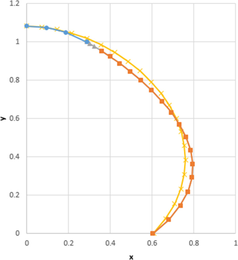
Meniscus of a water droplet (yellow line, on a solid plate without a hole; blue line, on an air-filled hole; and red line, on the solid part of a plate with an air-filled hole).

4. Conclusions

The Bézier curve method can be applied to approximately solve the Young–Laplace equation for various shapes of the meniscus of water formed under gravity, such as in a cylindrical capillary, beside one smooth plate, between two vertical plates, and as a sessile water drop on a smooth plate. The accuracy of the computation increases as the degree of the Bézier curve increases. The degree of the Bézier curve necessary to achieve sufficient accuracy within a certain range of the meniscus size, and the contact angle depends on where the meniscus is formed, that is, the 4th degree Bézier curve is required for the meniscus in a cylindrical capillary, beside one smooth plate, and between two vertical plates, while the 5th degree is required for the shape of a sessile drop on a smooth surface. By using straightforward optimization techniques, the solution can be easily obtained by the Bézier curve method without any sophisticated mathematical techniques.

This research did not receive any specific grant from funding agencies in the public, commercial, or not-for-profit sectors.

The authors declare no competing financial interest.

References

- Eslami F.; Elliott J. A. W. Gibbsian thermodynamic study of capillary meniscus depth. Sci. Rep. 2019, 9, 657. 10.1038/s41598-018-36514-w. [DOI] [PMC free article] [PubMed] [Google Scholar]
- Bullard J. W.; Garboczi E. J. Capillary rise between planar surfaces. Phys. Rev. E 2009, 79, 011604. 10.1103/physreve.79.011604. [DOI] [PubMed] [Google Scholar]
- Lobanov E. M. Shape and volume of liquid meniscus at the surface of a specimen. J. Eng. Phys. Thermophys. 2013, 86, 634–644. 10.1007/s10891-013-0877-0. [DOI] [Google Scholar]
- Biery J. C.; Oblak J. M.. A Calculational method for the determination of surface tensions with menisci-with application to water and mercury. University of California, Los Alamos Scientific Laboratory Report, August 28, 1964. [Google Scholar]
- Soligno G.; Dijkstra M.; van Roij R. The equilibrium shape of fluid-fluid interfaces: Derivation and a new numerical method for Young’s and Young-Laplace equations. J. Chem. Phys. 2014, 141, 244702. 10.1063/1.4904391. [DOI] [PubMed] [Google Scholar]
- Henriksson U.; Eriksson J. C. Thermodynamics of capillary rise: Why is the meniscus curved?. J. Chem. Edu. 2004, 81, 150–154. 10.1021/ed081p150. [DOI] [Google Scholar]
- Ward C. A.; Sasges M. R. Effect of gravity on contact angle: A theoretical investigation. J. Chem. Phys. 1998, 109, 3651–3660. 10.1063/1.476962. [DOI] [Google Scholar]
- Malijevský A.; Parry A. O. Edge contact angle, capillary condensation, and meniscus depinning. Phys. Rev. Lett. 2021, 127, 115703. 10.1103/physrevlett.127.115703. [DOI] [PubMed] [Google Scholar]
- Behroozi F. A fresh look at the Young-Laplace equation and its many applications in hydrostatics. Phys. Teach. 2022, 60, 358–361. 10.1119/5.0045605. [DOI] [Google Scholar]
- Liu S.; Li S.; Liu J. Jurin’s law revisited: Exact meniscus shape and column height. Eur. Phys. J. E: Soft Matter Biol. Phys. 2018, 41, 46. 10.1140/epje/i2018-11648-1. [DOI] [PubMed] [Google Scholar]
- Lv C.; Shi S. Wetting states of two dimensional drops under gravity. Phys. Rev. E 2018, 98, 042802. 10.1103/physreve.98.042802. [DOI] [Google Scholar]
- Tang Y.; Cheng S. The meniscus on the outside of a circular cylinder: From microscopic to macroscopic scales. J. Colloid Interface Sci. 2019, 533, 401–408. 10.1016/j.jcis.2018.08.081. [DOI] [PubMed] [Google Scholar]
- Eißman P. B.; Odenbach S.; Lange A. Meniscus of a magnetic fluid in the field of a current-carrying wire: Three-dimensional numerical simulations. Materials 2020, 13, 775. 10.3390/ma13030775. [DOI] [PMC free article] [PubMed] [Google Scholar]
- Liu J.; Sun J.; Mei Y. Biomimetic mechanics behaviors of the strider leg vertically pressing water. Appl. Phys. Lett. 2014, 104, 231607. 10.1063/1.4883493. [DOI] [Google Scholar]
- Liu J.; Sun J.; Liu L. Elastica of a pendant droplet: analytical solution in two dimension. Int. J. Non Lin. Mech. 2014, 58, 184–190. 10.1016/j.ijnonlinmec.2013.10.001. [DOI] [Google Scholar]
- Racz L. M.; Szekely J.; Brakke K. A. A general statement of the problem and description of a proposed method of calculation for some meniscus problems in materials processing. ISIJ Int. 1993, 33, 328–335. 10.2355/isijinternational.33.328. [DOI] [Google Scholar]
- O’Brien W. J.; Craig R. G.; Peyton F. A. Capillary penetration between dissimilar solids. J. Colloid Interface Sci. 1968, 26, 500–508. 10.1016/0021-9797(68)90298-1. [DOI] [Google Scholar]
- Morcos I. Determination of surface tensions of liquids from liquid meniscus rise on partially immersed plates. J. Chem. Phys. 1971, 55, 4125–4127. 10.1063/1.1676712. [DOI] [Google Scholar]
- Bashforth F.; Adams J.. An attempt to test the theories of capillary action by comparing the theoretical and measured forms of drops of fluid; Cambridge University, 1883. [Google Scholar]
- Dang Q.; Song M.; Luo X.; Qu M.; Wang X. A modeling study of different kinds of sessile droplets on the horizontal surface with surface wettability and gravity effects considered. Energy Storage Sav. 2022, 1, 22–32. 10.1016/j.enss.2021.11.002. [DOI] [Google Scholar]
- Srinivasan S.; McKinley G. H.; Cohen R. E. Assessing the accuracy of contact angle measurements for sessile drops on liquid-repellent surfaces. Langmuir 2011, 27, 13582–13589. 10.1021/la2031208. [DOI] [PubMed] [Google Scholar]
- Venkataraman P.Explicit solutions for linear partial differential equations using Bezier functions. In Proceedings of IDETC/CIE 2006 ASME 2006 International Design Engineering Technical Conferences & Computers and Information in Engineering Conference September 10-13: Philadelphia, Pennsylvania, USA, 2006.
- Ghomanjani F.; Hadi Farahi M. The Bezier control points method for solving delay differential equation. Intel. Contr. Autom. 2012, 03, 188–196. 10.4236/ICA.2012.32021. [DOI] [Google Scholar]
- Ghomanjani F.; Khorram E. Approximate solution for quadratic Riccati differential equation. J. Taibah Univ. Sci. 2017, 11, 246–250. 10.1016/j.jtusci.2015.04.001. [DOI] [Google Scholar]
- Ghomanjani F.; Shateyi S. A new approach for solving Bratu’s problem. Demonstr. Math. 2019, 52, 336–346. 10.1515/dema-2019-0023. [DOI] [Google Scholar]
- Sweitzer S.; Kumar T. K. S.. Differential Programming via OR Methods. In 27th International Conference on Principles and Practice of Constraint Programming (CP 2021); Michel L. D., Ed., 2021; pp 53:1–53:15. Article No. 53.
- Manikandan A.; Kamanat P. K. Laminar flow prediction over a rotating disc using Bezier curves. Int. J. Sci. Res. 2020, 9, 1767–1776. 10.21275/SR20525174309. [DOI] [Google Scholar]
- Narooei K.; Taheri A. K. Using of Bezier formulation for calculation of streamline, strain distribution and extrusion load in rectangular cross section of ECAE process. Int. J. Comput. Methods 2013, 10, 1350005. 10.1142/S0219876213500059. [DOI] [Google Scholar]
- Zheng J.; Sederberg T. W.; Johnson R. W. Least squares methods for solving differential equations using Bézier control points. Appl. Numer. Math. 2004, 48, 237–252. 10.1016/j.apnum.2002.01.001. [DOI] [Google Scholar]
- Tadmor R. Open problems in wetting phenomena: Pinning retention forces. Langmuir 2021, 37, 6357–6372. 10.1021/acs.langmuir.0c02768. [DOI] [PubMed] [Google Scholar]
- https://www.youtube.com/watch?v=uxsRW4KofUc (Accessed on Feb. 27, 2023).
- Lewis K.; Matsuura T. Calculation of the meniscus shape formed under gravitational force by solving the Young–Laplace differential equation using the Bézier curve method. ACS Omega 2022, 7, 36510–36518. 10.1021/acsomega.2c04359. [DOI] [PMC free article] [PubMed] [Google Scholar]
- Kung C. H.; Sow P. K.; Zahiri B.; Mérida W. Assessment and interpretation of surface wettability based on sessile droplet contact angle measurement: Challenges and opportunities. Adv. Mater. Interfaces 2019, 6, 1900839. 10.1002/admi.201900839. [DOI] [Google Scholar]
- Chou T. H.; Hong S. J.; Sheng Y. J.; Tsao H.-K. Wetting behavior of a drop atop holes. J. Phys. Chem. B 2010, 114, 7509–7515. 10.1021/jp100258m. [DOI] [PubMed] [Google Scholar]