Double Extended Kalman Filter Algorithm Based on Weighted Multi-Innovation and Weighted Maximum Correlation Entropy Criterion for Co-Estimation of Battery SOC and Capacity

Abstract

Most of the traditional extended Kalman filter algorithms for the co-estimation of SOC and capacity of lithium-ion batteries are designed based on the minimum mean square error (MMSE) criterion, which may show superior performance in Gaussian noise scenes. However, due to the complexity of the battery operating environment, it is likely to face non-Gaussian noise (especially outlier noise), at which time the performance of the traditional extended Kalman filter algorithms will be seriously weakened. To solve the above problems, this paper first proposes a double extended Kalman filter algorithm based on weighted multi-innovation and weighted maximum correlation entropy (WMI-WMCC–DEKF) for the co-estimation of battery SOC and capacity. In this paper, the performance of the target algorithm is verified and compared by generating different types of noise from three noise models: weak Gaussian mixture noise, strong Gaussian mixture noise, and outlier noise. The maximum absolute error value (MAE) and root mean square error value (RMSE) of the WMI-WMCC–DEKF algorithm can achieve the highest performance improvement of 69.3 and 84.2% (SOC), 61.3, and 94.2% (capacity), respectively. The experimental results fully prove that the target algorithm has excellent performance against three kinds of noises.

1. Introduction

With the intensification of the global energy crisis and the increasingly stringent carbon emission control in various countries, countries have begun to promote the use of new energy vehicles, mainly electric vehicles, to replace vehicles powered by fossil fuels.^1,2 Therefore, electric vehicles with low emissions and low noise are becoming popular products in the market.³ The power battery, as the core component of electric vehicles, has become the main battlefield of R&D and innovation of various automobile manufacturers. Lithium-ion batteries with high power density, long life, low memory, and wide operating temperature are gradually used as power batteries in electric vehicles.^4,5 To ensure the stable and reliable operation of the battery, the battery management system is required to monitor the internal state of the battery, such as SOC, SOH, and SOE.⁶

1.1. SOC Estimation

SOC is defined as the ratio of the current available capacity to the rated capacity of the battery.^7,8 SOC indicates the available capacity of the battery, which is closely related to the driving range of electric vehicles and is paid special attention by users.⁹ Generally, the main SOC prediction algorithms are divided into three categories:¹⁰ the first is open-loop algorithms; the second is model-based algorithms; and the third type is based on data-driven algorithms. As an open-loop algorithm, the ampere-hour integration method uses the relationship between current and SOC to predict SOC through integration. Due to the simple implementation of the ampere-hour integration method, a large number of battery management systems use this algorithm. However, the accuracy of this algorithm depends heavily on the accuracy of battery current and voltage data acquisition, as well as the accuracy of SOC initial value setting.¹¹ If the sensor has a certain deviation, with the cumulative effect of integration, there will be a big difference in the estimation algorithm. As another open-loop algorithm, the OCV-SOC look-up table algorithm establishes the OCV-SOV correspondence in advance offline and is usually used to calibrate the initial SOC value setting of the ampere-hour algorithm.^9,11 To overcome the shortcomings of open-loop prediction algorithms, model-based prediction algorithms with high accuracy and easy implementation have been proposed in large numbers.¹² These models include the electrochemical model, equivalent circuit model, single-particle model,⁹ etc. Based on the equivalent circuit model, the Kalman filtering algorithms and their extended algorithm with good real-time performance have been widely studied and applied.¹³ The extended Kalman filter is approximate to the linear system by Taylor series expansion of a nonlinear system, which is very suitable for real-time prediction of SOC, so it is widely used.¹⁴ In the equivalent circuit model, the accuracy of using the EKF algorithms to predict SOC depends heavily on the setting of noise variance, and inappropriate noise variance setting will degrade the performance of the algorithms and even cause the divergence of prediction results.¹⁵ Therefore, to solve the problem of noise variance setting, a large number of adaptive extended Kalman filtering algorithms have been proposed.¹⁶⁻²⁰ In the process of linearization of nonlinear systems, the second-order and higher terms are ignored in the results obtained by the Taylor series expansion of the extended Kalman filter, so there will be some errors in the results of the extended Kalman filter at the beginning. To solve the above problems, a large number of nonlinear Kalman filtering algorithms are proposed. A double Unscented Kalman filter algorithm with adaptive noise covariance to estimate battery SOC was proposed.²¹ A combination of a short-term memory network and an unscented Kalman filter was proposed to estimate battery SOC.²² The cubature Kalman filter algorithm was used to estimate SOC.²³⁻²⁵ A particle filter was proposed to estimate the SOC of battery.²⁶ Compared with the model-based SOC prediction algorithm, the data-driven algorithm only needs limited battery internal information.²⁷ The data-driven algorithms can be roughly divided into feedforward neural network algorithms, classification and regression algorithms, probabilistic algorithms, recurrent neural network algorithms, rule-based algorithms, hybrid algorithms,²⁸ etc. The author proposed a feedforward neural network with current, temperature, and polarization state as inputs for battery SOC estimation, which could achieve relatively accurate SOC estimation at low temperature and low SOC in the paper.²⁹ A radial basis function neural network with particle swarm optimization algorithm was used for battery state of charge estimation.³⁰ Lipu et al. used the gravitational search algorithm (GSA) to determine the optimal number of hidden layer neurons of the extreme learning machine (ELM) algorithm and estimated SOC through the improved ELM algorithm.³¹ A hybrid wavelet neural network algorithm combining discrete wavelet transform and adaptive wavelet neural network was proposed for battery SOC estimation.³² Hossain Lipu et al. proposed a time-delay neural network algorithm for estimating the state of charge of lithium-ion batteries, which used the firefly algorithm to optimize hidden neurons and input time-delay parameters.³³ Chemali et al. proposed a deep feedforward neural network (DFNN), which used data under different temperatures and scenes for training so that the measured battery-related data could be directly mapped to SOC through the network in the paper.³⁴ A support vector machine algorithm with data classification and dataset size optimization was proposed for SOC prediction.³⁵ A stacked bidirectional long short-term memory (SBLSTM) neural network was proposed for SOC estimation of lithium-ion batteries.³⁶ Ren et al. proposed to use a particle swarm optimization algorithm to optimize the parameters of long and short memory network for battery SOC estimation.³⁷ Although the above data-driven intelligent algorithms can obtain accurate battery SOC estimates without relying on accurate battery models, these algorithms have high requirements for training data and quality, which often limit the application of these intelligent algorithms in the real-time estimation of battery SOC.²

1.2. SOH Estimation

SOH is an indicator used to predict the aging state of the battery, which is defined as the ratio of the current maximum capacity to the rated capacity of the battery.⁸ Algorithms for predicting SOH are generally divided into two categories: model-based algorithms and data-driven algorithms.⁵ The most direct method to estimate SOH is to directly test the capacity and internal resistance of the battery³⁸⁻⁴⁰ and use these two parameters to evaluate the aging degree of the battery. However, due to the uncertainty of the operating environment, the accuracy of SOH estimation may not be guaranteed. Based on the battery model. The authors proposed an unscented Kalman filter algorithm and particle Kalman filtering algorithm, respectively, to estimate SOH.⁴¹ However, it is difficult to obtain an accurate battery model due to the complex chemical reaction inside the battery and the external working environment.⁴² Therefore, data-driven algorithms with low dependence on models have been widely concerned and applied. In general, the data-driven algorithm uses the battery’s historical degradation data and battery status monitoring data including current, voltage, and temperature to mine the current battery health status information, thus realizing the prediction of SOH.⁴³ These data-driven algorithms can be roughly divided into algorithms based on the artificial neural network,^44,45 algorithms based on support vector machine,^46,47 Gaussian process regression (GPR),⁴⁸ etc. In addition, there are some hybrid algorithms. Song et al. proposed a combination of an unscented particle filter and least squares support vector machine (LS–SVM) to estimate SOH.⁴⁹ Sun et al. proposed a joint algorithm of unscented particle filter and optimized multi-kernel relevance vector machine (OMKRVM) to estimate the SOH of the battery in the paper.⁵⁰ Considering the interference of external noise, the algorithm first used the initial value and actual capacity estimated by the UPF to calculate the error, and then used the complementary ensemble empirical mode decomposition (CEEMD) to reconstruct the residual. Then, the OMKRVM algorithm with optimized kernel parameters and weights was used to correct the initial predicted value. Chen et al. proposed an algorithm combining self-reviewing moving average and Elman neural network to achieve SOH estimation.⁵¹ The above data-driven algorithms need to spend a lot of time training the network and have certain requirements for data and quality.

1.3. Joint Estimation of SOC and SOH

Battery state SOC and SOH, as well as other state variables, are often closely coupled.⁵² Therefore, many scholars focus on the joint estimation of multiple states. For the need for real-time battery state estimation, a large number of model-based algorithms have been proposed. To make full use of the error information sequence and residual information sequence, the author proposed an improved double adaptive extended Kalman filter based on the dynamic window to estimate battery state SOC and SOH.²⁰ Xiao et al. proposed a simplified decoupled joint estimation algorithm of SOC and SOH based on convex optimization to solve the problem that the high coupling of SOC and SOH would lead to the complexity of the designed observer.⁴ When calculating SOC, the algorithm did not need the traditional Coulomb calculation method, to realize the decoupling between SOC and battery capacity and ultimately reduce the complexity of observer and algorithm design. Based on the first-order RC model, the author used the forgetting factor least squares to identify the model parameters and then used the double adaptive extended Kalman filter to estimate the SOC and battery capacity.⁵³ Aiming at the problem that it was difficult to guarantee prediction accuracy when SOC and SOH were estimated at the same time, the author proposed a sequential algorithm that used frequency-scale separation and sequential parameter/state estimation by injecting currents of different frequencies, and then used double extended Kalman filter to achieve the estimation of SOC and SOH.⁵⁴ Generally, the battery state SOC is a fast variable, while the battery capacity is a slow variable. Therefore, some authors have proposed a multiscale estimation algorithm for this situation, the micro time scale to estimate SOC and the macro time scale to update capacity.^55,56 However, in the iterative calculation process of the above algorithms, the noise was assumed to be Gaussian noise, and the minimum mean square estimation criterion was used to obtain the iterative prediction algorithm. However, the battery operating environment is very complex, and there may be non-Gaussian noise, so it is necessary to study how to predict the algorithm in the complex noise environment. To solve the above problems, some scholars began to study prediction algorithms that were robust to non-Gaussian noise. Among them, algorithms based on the correlation entropy criterion are widely used in various fields. The entropy-based Kalman filter algorithm is used for satellite attitude estimation and global satellite navigation, respectively.^57,58 By introducing a new gain matrix, the author extended the maximum correlation entropy criterion Kalman filter to the distributed algorithm to form the distributed maximum correlation entropy Kalman filter (D-MCKF) in the paper.⁵⁹ On the basis of the traditional extended Kalman filter, the author used the maximum correlation entropy criterion to replace the minimum mean square criterion in the traditional extended Kalman filter, thereby proposing the maximum correlation entropy extended Kalman filter (MCEKF) algorithm suitable for non-Gaussian environments.⁶⁰ For ultrasonic positioning, a maximum correlation entropy criterion extended Kalman filter weighted centroid location algorithm was proposed for ultrasonic location.⁶¹ According to the statistics of the published literature and research results, only one paper,³ the maximum correlation entropy extended Kalman filter algorithm was used to estimate the battery SOC. Therefore, this paper is the first time to use the double extended Kalman filter algorithm based on the weighted multi-innovation and weighted maximum correlation entropy criterion to jointly estimate the SOC and capacity of the battery. The main contributions of this paper are as follows:

• (1)In this paper, the cost function of battery parameter identification is constructed based on the maximum correlation entropy for the first time, and the calculation steps of the parameter estimation algorithm are derived;
• (2)In view of the influence of non-Gaussian noise, this paper takes maximum correlation entropy as the criterion, and on the basis of the weighted maximum correlation entropy extended Kalman filtering algorithm (WMCC-EKF), proposes the weighted multi-innovation and weighted maximum correlation entropy extended Kalman filtering algorithm (WMI-WMCC-EKF);
• (3)On the basis of the WMI-WMCC-EKF algorithm, a double extended Kalman filter algorithm based on weighted multi-innovation and weighted maximum correlation entropy (WMI-WMCC–DEKF) is proposed for the co-estimation of battery SOC and capacity;
• (4)A variety of noise models are constructed to simulate different kinds of mixed noise;
• (5)The algorithm proposed in this paper has been tested with data of different types of working conditions containing different kinds of noise, and the superior performance of the algorithm proposed in this paper has been proved.

The rest of this paper is organized as follows: In Section 2, the battery model and parameter identification are analyzed, in which the parameter identification algorithms based on the least squares error criterion and the maximum correlation entropy criterion are derived and compared in detail. In Section 3, the WMI-WMCC–DEKF algorithm for co-estimation of battery SOC and capacity is proposed; In Section 4, by constructing different noise generation models, the target algorithm proposed in this paper is tested under various noise conditions, and the performance of different algorithms is quantitatively compared; In Section 5, the paper is summarized.

2. Battery Model and Parameter Identification

2.1. Battery Model

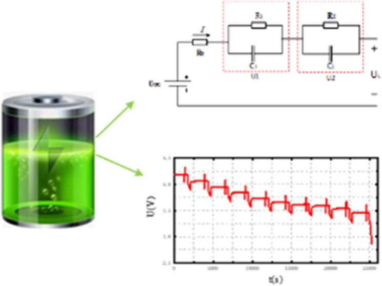
As previously analyzed, the equivalent circuit model (ECM) is widely used in battery modeling because it can better simplify the description of the internal dynamic process of the battery, and the accuracy of the equivalent circuit often depends on the order of the equivalent model and the accuracy of the parameters. The second-order Thevenin model formed by adding an RC circuit to the Rint model can achieve a good balance between accuracy and computation, and can better describe the diffusion effect and charge transfer effect inside the battery. The circuit block diagram of the model is shown in Figure 1.

Figure 1.

Second-order Thevenin model.

In the above model, U_oc represents the open-circuit voltage; R_o represents the internal resistance of the battery; U_L represents terminal voltage; I represents the current in the equivalent circuit (when the battery is discharged, the current direction is positive); U₁ represents the voltage at both ends of R₁ and C₁; U₂ is equal to the voltage at both ends of R₂ and C₂; R₁ and R₂ represent the electrochemical polarization impedance and central polarization impedance inside the battery, respectively; and C₁ and C₂ represent the electrochemical polarization capacitance and central polarization capacitance inside the battery, respectively. Based on Kirchhoff’s law, the circuit equivalent expression can be expressed as follows

1

2

3

2.2. Parameter Identification

To estimate the SOC and capacity of the battery, it is important to identify the parameters in the equivalent circuit model. At present, most parameter identification algorithms are derived based on the least squares error criterion under Gaussian noise.

2.2.1. Parameter Identification Based on Least Square Criterion

At present, most parameter identification algorithms assume that under the Gaussian noise environment, the least squares error criterion is used to realize parameter identification. It is assumed that the system equation of the n-order system is eq 4, and the parameter discretization expression to be identified is eq 5.

4

5

Eq 5 can be further expressed as the following equation

6

In eq 6, ϕ(k) = [−y(k – 1), −y(k – 2),···, −y(k – n), u(k – 1), u(k – 2),···, u(k – n)]

θ = [a₁, a₂,···, a_n, b₁, b₂,···, b_n]. Based on the least squares error criterion, take the cost function as J(θ), then

7

To obtain the optimal parameter θ, to minimize J(θ), the derivative of the cost function J(θ) with respect to θ can be obtained

8

9

10

Assuming the full rank of the system, the estimated parameters can be obtained as shown in eq 11.

11

2.2.2. Maximum Correlation Entropy Criterion

As a local similarity measurement, correlation entropy is not very sensitive to outliers and noise, so it is widely used in ultrasonic positioning,⁶¹ complex network control,⁶² power system state tracking,⁶³ and other fields. The definition of correlation entropy⁶⁴ is as follows

12

13

where V_σ(X, Y) represents the correlation entropy between variables X and Y, E represents the expected operation factor, K_σ(x, y) is a continuous positive kernel function with a kernel width of σ, and ρ_XY(x, y) is the joint probability density function of x and y. Unless otherwise stated, the kernel function used in this paper is the Gaussian kernel function expressed in eq 14

14

In eq 14, e = x – y, σ (>0) is the kernel width, which is taken as 0.5 in this paper. In practice, the joint probability density ρ_XY(x, y) between variables x and y is usually unknown, and the available measurement data is also limited. Therefore, the entropy between variables X and Y is often predicted by the mean value of the sampling value, as shown in eq 15.

15

In eq 15, x_i and y_i are the ith sampling values of random variables X and Y, respectively, and N is the total number of samples. For the Gaussian kernel function G_σ(e), a very important feature is when e = 0, that is X = Y, the Gaussian kernel function will reach its maximum value. Through Taylor series expansion of the correlation entropy function, it can be found that the correlation entropy is the weighted sum of random variables of X – Y each order,⁶⁴ and the expression is shown in eq 16.

16

It can be seen from eq 16 that the correlation entropy is the weighted sum of the even moments of each order, and the correlation entropy can obtain the high-order information of the random variables. Especially when the kernel bandwidth σ takes a larger value, the second-order moment will play a major role in the correlation entropy. Therefore, when the statistical data of random variables X and Y are finite N, assuming that the error data {e_i}_i = 1^N between them is available, the cost function based on the maximum correlation entropy criterion is defined as

17

2.2.3. Parameter Identification Based on Maximum Correlation Entropy Criterion

Similar to parameter identification based on the least mean square error criterion, it is assumed that the system and parameter expressions to be identified are shown in eq 18.

18

Under the maximum correlation entropy criterion, for real-time data, the cost function corresponding to eq 18 can be expressed as eq 19.

19

To obtain the best estimation parameter in eq 19, it is necessary to obtain the derivative of the expression concerning variable θ and make it zero. The relevant calculation process is as follows

20

21

22

In eq 22, and 1/σ² are constant values, respectively, so eq 22 can be further simplified

23

When the system is in full rank, the parameter estimates obtained are shown in eq 24.

24

By comparing eqs 11 and 24, it can be found that the parameter estimates under the maximum correlation entropy criterion are consistent with those under the least squares error criterion.

2.2.4. Parameter Identification of Second-Order Thevenin Model

To identify the parameters of the second-order Thevenin model used in this paper, we S transform eqs 1–3 to obtain eq 25.

25

Let τ₁ = R₁C₁, τ₂ = R₂C₂, a = τ₁τ₂, b = τ₁ + τ₂, d = R₁τ₂ + R₂τ₁ + R₀(τ₁ + τ₂), c = R₁ + R₂ + R₀, then there is eq 26.

26

Using s = [x(k) – x(k – 1)]/T_s and s² = [x(k) – 2x(k – 1) + x(k – 2)]/T_s² to discretize eq 26, the expression described by eq 27 can be obtained

27

where y(k) = U_OC(k) – U_L(k), m₁ = (−bT_s – 2a)/(T_s² + bT_s + a), m₂ = a/(T_s + bT_s + a), m₃ = (cT_s² + dT_s + aR₀)/(T_s + bT_s + a), , and , and eq 27 can be transformed into the discrete difference expression described in eq 28.

28

Eq 28 can be further written into the equation of state described in eq 29.

29

where ϕ(k) = (−y(k – 1), −y(k – 2), I(k), I(k – 1), I(k – 2)); this paper obtains parameter estimation θ = (m₁, m₂, m₃, m₄. m₅)^T through an iterative least square algorithm with forgetting factor shown in eq 30,⁵⁶ which is used to obtain the estimated values of each parameter of the second-order Thevenin model.

30

3. Double Extended Kalman Filter Algorithm Based on Weighted Multi-Innovation and Weighted Maximum Correlation Entropy Criterion (WMI-WMCC–DEKF) for Battery State of Charge and Capacity Estimation

3.1. Extended Kalman Filtering Algorithm Based on the Weighted Maximum Correlation Entropy Criterion (WMCC-EKF)

The traditional EKF algorithms based on the minimum mean square error criterion are widely used in battery state estimation because of their good real-time performance and computational simplicity in the Gaussian noise environment. For the traditional EKF algorithms, such as the simplified nonlinear system described in eq 31, it is necessary to use the Taylor series to linearize the functional equations R(·) and S(·) to obtain and , and can work normally only if the system noise w_k and r_k are Gaussian noise.

31

If the noise w_k and r_k of the system are non-Gaussian noise, it is difficult for the traditional EKF algorithm to obtain the estimator with high accuracy, and there are some cases that it cannot work properly. In ref (65), the maximum correlation entropy cost function is used to replace the minimum mean square error cost function commonly used in Gaussian noise environments so that the filtering algorithm has good filtering performance in non-Gaussian environments. To further strengthen the robustness of the maximum correlation entropy extended Kalman filter, the weighted maximum correlation entropy cost function is used to replace the maximum correlation entropy cost function, Thus, the filtering algorithm has better filtering performance in non-Gaussian environment. In refs (65, 66), the author proposed the expression of the cost function of the single-point weighted maximum correlation entropy when N = 1, as shown in eq 32.

32

To obtain the optimal estimate value x̂_k, it is necessary to take the derivative of the eq 32 with respect to x̂_k and set it to zero. The complete calculation process is as follows

33

34

35

where

36

Add or subtract an item L_kH_k^TR_kH_kx̂_k^– on the right side of eq 35, then there is:

37

38

39

From eq 39, it can be obtained that:

40

where:

41

Therefore, the main steps of the WMCC-EKF algorithm are as follows:

Initialization:

42

43

Prediction step:

44

45

Update step:

46

47

48

If the WMCC-EKF algorithm is mapped to a closed-loop control loop with feedback, its block diagram is shown in Figure 2:

Figure 2.

Closed-loop control loop corresponding to the WMCC-EKF algorithm.

3.2. Extended Kalman Filter Algorithm Based on Weighted Multi-Innovation and Weighted Maximum Correlation Entropy Criterion (WMI-WMCC-EKF)

To further improve the performance of the WMCC-EKF algorithm, we added a weighted multi-innovation computing unit in the closed-loop control loop corresponding to the WMCC-EKF. This unit can further improve the estimation accuracy of the algorithm by storing and weighting the error innovation and gain with the length of N, and converting the traditional single-innovation-adjusted estimator into a weighted multi-innovation-adjusted estimator. The corresponding structure diagram is shown in Figure 3:

Figure 3.

Closed-loop control loop corresponding to the WMI-WMCC-EKF algorithm.

In the weighted multi-innovation calculation control unit corresponding to Figure 3, the expression corresponding to the error matrix E_N (k) is shown in eq 49, the expression corresponding to the gain matrix is shown in eq 50, and N is the length of innovation calculation.

49

50

Then, the estimation adjustment algorithm corresponding to the WMI-WMCC-EKF algorithm is as follows:

51

52

53

In eq 53, λ ∈ [0, 1], λ is taken as 0.5 in this paper. The complete calculation steps and processes based on the WMI-WMCC-EKF algorithm are shown in Figure 4:

Figure 4.

Calculation steps and flow of the WMI-WMCC-EKF algorithm.

3.3. Double Extended Kalman Filter Algorithm Based on Weighted Multi-Innovation and Weighted Maximum Correlation Entropy Criterion (WMI-WMCC–DEKF) for Co-Estimation of Battery SOC and Capacity

Among the relevant characteristics of battery, SOC and capacity are two important status indicators of battery. SOC reflects the remaining capacity of battery, which is directly related to the use time of battery. The capacity of the battery is related to the health state of the battery and reflects the aging state of the battery. SOC is a relatively fast-changing quantity, while the change of battery capacity closely related to battery life is relatively slow. Therefore, when simultaneously predicting the SOC and capacity of batteries, double EKF is often used for prediction, and the fast and slow time scales are distinguished.

3.3.1. Definition of SOC and Capacity

SOC is used to represent the available capacity of the current battery, which is defined as follows:⁵⁶

54

55

In eq 54, SOC(t) is the state of charge value of the battery at the time t and SOC(t₀) is the initial value of the corresponding state of charge; C_max is the rated maximum usable capacity of the new battery, which will gradually decline with the use of the battery; η is the coulomb efficiency associated with battery charging and discharging; and i(t) is the load current of the battery (the current direction is negative when charging and positive when discharging). After discretization of eq 54, the discrete expression expressed in eq 55 is obtained; SOC_k represents the current time value of SOC; C_k,max represents the current maximum usable capacity; and T_s represents the sampling period of the discrete system.

3.3.2. WMI-WMCC–DEKF Algorithm for Co-Estimation of Battery SOC and Capacity

For two random variables X and θ, the corresponding double EKF state space model can be written as follows

56

In eq 56, θ_k and X_k are two random variables to be estimated; Y_k is the observation; f() is a function in the equation of state; g() is a function in the observation equation; v_k, w_k, and r_k are noise with zero mean and covariance Q_θ, Q_X, and R_X, respectively; A_k, B_k, H_k, and D_k are the corresponding coefficient matrices of each variable. In this paper, the battery capacity C is taken as the estimator θ. While SOC, the terminal voltages U_P1 and U_P2 of C₁ and C₂ are taken as components of the estimator X. Therefore, the discrete state space model of the battery can be expressed as follows

57

It can be concluded from eq 57 that the SOC of the battery is closely related to the capacity C of the battery, so the prediction of C is also very necessary. However, compared with the change speed of battery SOC, the attenuation speed of battery capacity C is slow, so it is not necessary to predict every time, but at intervals. Therefore, the double extended Kalman filter in this paper is divided into two parts: micro prediction and macro prediction.⁵⁶ The micro Kalman filtering algorithm uses the battery terminal voltage as the value of observation Z_X,k. In ref (67), the author takes the SOC estimated from the state equation as the observation value of the macro Kalman filtering algorithm. In this paper, the macro Kalman filtering algorithm uses the SOC estimated from the micro Kalman filtering as the value of the observation Z_C,k, and its interval length is L. On the basis of the WMI-WMCC-EKF, for the discrete state model eq 57, we can get the calculation process of the WMI-WMCC–DEKF for the co-estimation of SOC and capacity as follows:

3.3.2.1. Micro Extended Kalman Filter for State Estimation

• (1)
  When k = 0, initialize the parameter:

  58

  59
• (2)Repeat the following steps when k = 1, 2, 3···:
• (3)
  Predict state variable X̂_k^– and covariance P_X,k|k–1:

  60

  61
• (4)
  Weighted multi-innovation calculation (in ref (66), in the calculation of L_X,k, approximate treatment is taken for the kernel function so that X̂_k ≈ X̂_k^–):

  62

  63

  64

  65

  66

  67
• (5)Update the estimator and covariance:

68

69

where A_k = [1 0 0; 0 e^–T_s/τ₁ 0; 0 0 e^–T_s/τ₂]; ; and D_k = [−R₀].

3.3.2.2. Macro Extended Kalman Filter for Parameter Estimation

• (1)
  When k = 0, initialize the parameter:

  70

  71
• (2)Repeat the following steps when k = 1. 2. 3···:
• (3)
  Predict state variable Ĉ_k^– and covariance P_C, k|k–1:

  72

  73
• (4)
  Update gain matrix K_C,k:

  74
• (5)Update the estimator and covariance:

75

76

The corresponding coefficient matrix is

The co-estimation algorithm proposed in this paper first uses the collected voltage and current data to complete the offline identification of the parameters of the second-order Thevenin model using the FFRLS algorithm. The forgetting factor in the FFRLS algorithm in this paper is 0.9998. Then, the proposed WMI-WMCC–DEKF algorithm is used to jointly estimate the battery’s SOC and capacity in the data with non-Gaussian noise. In the estimation process, first, the capacity Ĉ_k^– predicted in the macro Kalman filter is used in the micro Kalman filter (WMI-WMCC-EKF). In the WMI-WMCC-EKF algorithm, compared with the existing WMCC-EKF algorithm, the weighted multi-information control unit is added. The weighted multi-innovation control unit adjusts the estimated quantity by weighting and summing N innovations to form a new estimated quantity increment value. The SOC value estimated by the WMI-WMCC-EKF algorithm is used as the observation value of the observation equation of the macro Kalman filter algorithm to estimate the battery capacity. Because the collected battery terminal voltage is affected by the non-Gaussian noise much more than the current during the test, this paper mainly adds various types of noise to the terminal voltage. In addition, because the observed value used for battery capacity estimation is from the estimated SOC value in the WMI-WMCC-EKF, the non-Gaussian noise response is small. Therefore, the traditional extended Kalman filter algorithm is used in the macro Kalman filter algorithm, which can optimize the calculation time of the algorithm while maintaining the algorithm’s performance. The block diagram of the WMI-WMCC–DEKF algorithm for co-estimation of battery state of charge and capacity proposed in this paper is shown in Figure 5.

Figure 5.

Block diagram of the WMI-WMCC–DEKF for co-estimation of battery SOC and capacity.

4. Experimental Analysis

4.1. Experimental Test Platform

To verify the performance of the algorithm proposed in this paper, this paper uses the test platform shown in Figure 6. The platform consists of four parts. One part is the lithium-ion battery used in the test. The rated capacity of the battery is 70 Ah, but after a period of use, there is some aging (the current maximum capacity is 69.59 Ah). The second part is the temperature control box, which is used to generate a constant test temperature. The third part is the battery test system, which is produced by Shenzhen Yakeyuan Technology Co., Ltd., with the maximum voltage of 200 V, the maximum current of 100 Å, and the maximum charge, and discharge power of 750 W. The fourth part is the main computer control system, which is used to set the working conditions and store the data generated by the battery test system charging and discharging. In particular, the tests in this paper are carried out at room temperature. Here, we are especially grateful for the equipment and data provided by the New Energy Measurement and Control Laboratory of Southwest University of Science and Technology.

Figure 6.

Battery test platform.

4.2. Comparison Data and the Open-Circuit Voltage Fitting Method Used in This Paper

In this paper, it is assumed that the collected data source is stable and reliable with low noise, and the SOC data for comparison is obtained by using eq 55. The open-circuit voltage is closely related to SOC and can be fitted with the following polynomial function.

77

where f() represents the functional relationship between SOC and U_OC, and {m_i}_i = 0ⁿ is the coefficient of corresponding items. In this paper, n is taken as 5.

4.3. Comparison Algorithm and Evaluation Criteria Used in This Paper

To better compare the performance of the algorithm proposed in this paper, this paper uses the DEKF algorithm suitable for Gaussian noise as the comparison algorithm and also uses the WMCC–DEKF algorithm which is insensitive to non-Gaussian noise as the comparison algorithm. To compare the performance of three algorithms (WMI-WMCC–DEKF, WMCC–DEKF, and DEKF), this paper uses the maximum absolute error (MAE) and root mean square error (RMSE) to evaluate the algorithm performance. The specific expression of the two algorithms is shown in the following equation.

78

79

4.4. Noise Model Used in This Paper

To evaluate the performance of the target algorithm in the environment with non-Gaussian noise and outliers, this paper generates the corresponding noise through simulation and then adds the generated noise to the measured terminal voltage. According to the noise generation model in ref (66), the model used in this paper is as follows:

• (1)Weak mixture Gaussian noise model

80

In eq 80, μ₁ = 0.001, Q₁ = 0.0006, μ₂ = 0, Q₂ = 0.006, and a = 0.25. This model is used to simulate the mixed Gaussian noise with weak noise, and the noise signal generated is shown in Figure 7.

• (2)Strong mixture Gaussian noise model

81

Figure 7.

Weak mixed Gaussian noise.

In eq 81, μ₃ = 0, Q₃ = 0.005, μ₄ = 0, Q₄ = 0.05, and a = 0.5. This model is used to simulate the mixed Gaussian noise with strong noise, and the corresponding noise signal generated is shown in Figure 8.

• (3)Noise model with outliers

82

Figure 8.

Strong mixed Gaussian noise.

In eq 82, μ₅ = 0, Q₅ = 0.0002, to simulate the extreme outliers, that is, the continuous outliers occur, outliers take a small segment of larger random values. The noise signal generated by this model is shown in Figure 9.

Figure 9.

Noise with outliers.

4.5. Test the Target Algorithm Using HPPC Working Condition Data with Mixed Gaussian Noise

Although the WMI-WMCC–DEKF algorithm and WMCC–DEKF algorithm based on the maximum entropy criterion are mainly designed for the presence of non-Gaussian noise, the target algorithm works normally as the extended Kalman filter algorithm based on the minimum mean square error criterion under Gaussian noise. To compare the performance of the three algorithms, parameters of the battery model are first identified by offline FFRLS, and then WMI-WMCC–DEKF, WMCC–DEKF, and DEKF algorithms are used to estimate the SOC and capacity of the battery with HPPC working condition data without added noise. The results are shown in Figure 10, and the corresponding performance index statistics are shown in Tables 1 and 2.

Figure 10.

Results of co-estimation of SOC and capacity by three algorithms using HPPC working condition data without additional noise.

Table 1. Performance Indicators of Three Algorithms for SOC Estimation Using HPPC Working Condition Data with Different Types of Noise.

	no added noise		noise1		noise2
HPPC	MAE	RMSE	MAE	RMSE	MAE	RMSE
DEKF	0.1988	0.0170	1.6453	0.1278	1.3241	0.2905
WMCC–DEKF	0.1277	0.0101	0.1290	0.0099	0.1318	0.0101
WMI-WMCC–DEKF	0.0414	0.0015	0.0410	0.0013	0.0405	0.0016

Table 2. Performance Indicators of Three Algorithms for Capacity Estimation Using HPPC Working Condition Data with Different Types of Noise (the Unit of MAE and RMSE Is Ah).

	no added noise		noise1		noise2
HPPC	MAE	RMSE	MAE	RMSE	MAE	RMSE
DEKF	0.2737	0.0200	2.1600	0.1889	1.5494	0.2516
WMCC–DEKF	0.1392	0.0121	0.1417	0.0121	0.1448	0.0121
WMI-WMCC–DEKF	0.0575	7.1290 × 10–4	0.0573	7.1355 × 10–4	0.0560	7.0518 × 10–4

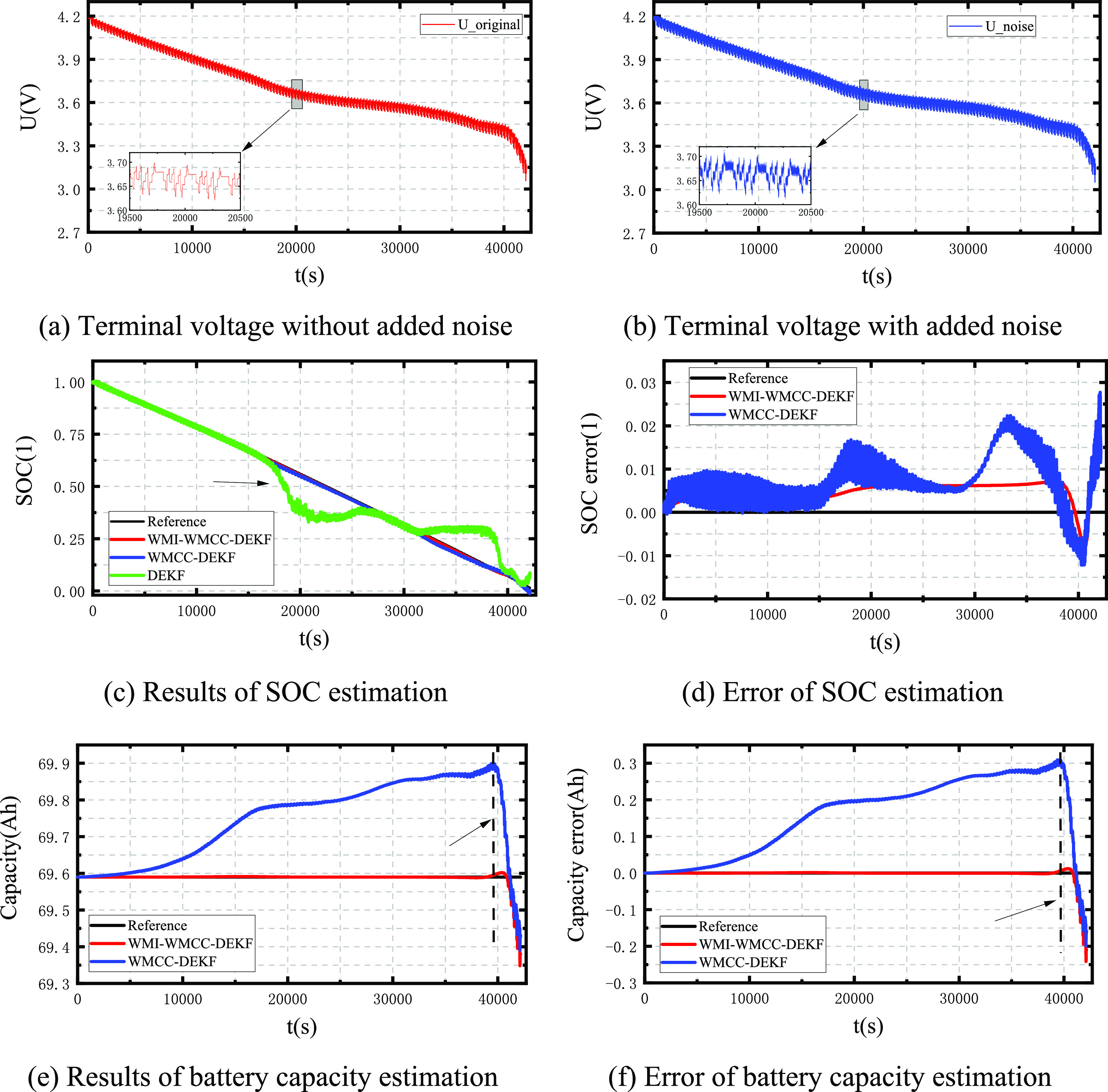
4.5.1. Performance of Target Algorithm in Processing Data without Additional Noise

First, test the performance of the three algorithms using the voltage and current without adding noise (as shown in Figure 10a and b) under HPPC working condition, and the results are shown in Figure 10. As can be seen from Figure 10c, for HPPC data containing ordinary Gaussian noise, the three algorithms can complete the SOC estimation well. From the local zoom of the arrow in Figure 10c, it can be seen that the estimated value of SOC by the DEKF algorithm fluctuates greatly, and the difference with the reference SOC value is large. However, the estimated SOC value of the WMCC–DEKF algorithm is closer to the reference value than that of the DEKF algorithm but worse than that of the WMI-WMCC–DEKF algorithm, which can also be analyzed from Figure 10d. In the statistical chart of SOC estimation error shown in Figure 10d, it is obvious that the SOC estimation error value of the WMI-WMCC–DEKF algorithm is much smaller than that of the WMCC–DEKF algorithm and the DEKF algorithm. In the specific indicators, it can be concluded from Table 1 that in the process of SOC estimation, the MAE and RMSE values of the WMI-WMCC–DEKF algorithm are 0.0414 and 0.0015, respectively, while the MAE and RMSE values of the WMCC–DEKF algorithm are 0.1277 and 0.0101. The WMI-WMCC–DEKF algorithm is 67.6 and 85.1% less than the WMCC–DEKF algorithm, respectively; The MAE and RMSE values of the DEKF algorithm are 0.1988 and 0.0170, and the WMI-WMCC–DEKF algorithm is 79.2 and 91.2% lower than the DEKF algorithm, respectively. The above analysis shows that the WMI-WMCC–DEKF algorithm proposed in this paper has the optimal SOC estimation performance among the three algorithms in the Gaussian noise environment. In the estimation of battery capacity, we can see from Figure 10e,f that the battery capacity estimated by the WMI-WMCC–DEKF algorithm is very close to the actual battery capacity of 69.59 Ah, with the smallest estimation error. However, there is a large deviation between the estimated battery capacity of the DEKF algorithm and the actual value, and the error fluctuation is very frequent, indicating that its dynamic tracking performance is weak compared with the other two algorithms. The end pointed out by the arrows in Figure 10e,f corresponds to the low SOC region of the battery. Due to the intensification of the electrochemical reaction inside the battery and the nonlinear relationship between SOC and U_OC, there will be a large estimation error in this region. The three algorithms will have a certain estimation error here. In Table 2, the MAE and RMSEs of the WMI-WMCC–DEKF algorithm are 58.7 and 94.1% lower than those of the WMCC–DEKF algorithm and 79 and 96.4% lower than those of the DEKF algorithm, respectively, in the statistical indicators for battery capacity estimation of the three algorithms. Based on the above analysis, the performance of the WMI-WMCC–DEKF algorithm is far better than the other two algorithms for the co-estimation of SOC and capacity under Gaussian noise.

4.5.2. Performance of Target Algorithm in Processing Data with Weak Gaussian Mixture Noise

In order to test the performance of the three algorithms under HPPC conditions with weak mixed Gaussian noise added, weak mixed Gaussian noise was added to the terminal voltage data as shown in Figure 11a to obtain the terminal voltage data with weak mixed Gaussian noise (as shown in Figure 11b). Comparing Figure 11a and b, it can be found that the disturbance of terminal voltage with mixed Gaussian noise increases. The estimated results of the three algorithms on the battery SOC and capacity are shown in Figure 11c–f, and the specific performance statistics indicators are shown in Tables 1 and 2. In Figure 11c, we can see that both the WMI-WMCC–DEKF algorithm and the WMCC–DEKF algorithm can estimate SOC. However, the DEKF algorithm does not work properly, indicating that the DEKF algorithm is very sensitive to weak mixed Gaussian noise. In the following performance comparison, only the WMI-WMCC–DEKF and the WMCC–DEKF are compared. In Figure 11d, except for the estimated value at the tail end, the estimation error of the WMI-WMCC–DEKF algorithm is very stable in the whole region and is far less than the estimation error of the WMCC–DEKF algorithm. In Table 1, the MAE and RMSE values of the WMI-WMCC–DEKF algorithm are 0.0410 and 0.0013, respectively, while the MAE and RMSE values of the WMCC–DEKF algorithm are 0.1290 and 0.0099, respectively. The former algorithm is 68.2 and 86.9% lower than the latter algorithm. For capacity estimation, since SOC estimated by each algorithm is used as the measured value, the accuracy of SOC estimated by each algorithm directly determines the accuracy of capacity estimation, which can be obtained from Figure 11e,f. In Figure 11e,f, except for individual tail estimates, the capacity estimated by the WMI-WMCC–DEKF algorithm is almost the same as the real value. The capacity estimation error of the WMCC–DEKF algorithm is larger than that of the WMI-WMCC–DEKF algorithm. For specific indicators, we can draw from Table 2 that in the capacity estimation process, the MAE and RMSE values of the WMI-WMCC–DEKF algorithm are 0.0573 and 0.00071355, respectively, while the MAE and RMSE values of the WMCC–DEKF algorithm are 0.1417 and 0.0121, respectively. The WMI-WMCC–DEKF algorithm is 59.6 and 94.1% lower than the WMCC–DEKF algorithm. It can be seen from the above analysis that, in the presence of weak mixed Gaussian noise, the WMI-WMCC–DEKF algorithm can more effectively resist noise interference than the other two algorithms and can accurately estimate the battery SOC and capacity.

Figure 11.

Results of co-estimation of SOC and capacity by three algorithms using HPPC working condition data with weak mixed Gaussian noise.

4.5.3. Performance of Target Algorithm in Processing Data with Strong Gaussian Mixture Noise

To simulate the environment with strong noise, the second kind of mixed Gaussian noise is added to the HPPC working condition data (As shown in Figure 12b), and then three algorithms are used to estimate the SOC and battery capacity of the battery. The results are shown in Figure 12c–f, and the statistics of the estimated performance indicators of the three algorithms are shown in Tables 1 and2. It can be concluded from Figure 12c that under the interference of strong mixed Gaussian noise, the WMI-WMCC–DEKF algorithm and the WMCC–DEKF algorithm can achieve the estimation of battery SOC, while the DEKF algorithm cannot work normally. Therefore, the performance of the previous two algorithms will be mainly analyzed later. It can be seen from Figure 12d that, except for the tail outlier pointed by the arrow, the SOC estimation error of the WMI-WMCC–DEKF algorithm is far less than the SOC estimation error of the WMCC–DEKF algorithm, showing superior anti-interference performance. As for the specific performance indicators of SOC estimation, we can draw from Table 1 that the MAE and RMSE values of the WMI-WMCC–DEKF algorithm are 0.0405 and 0.0016, respectively, while the MAE and RMSE values of the WMCC–DEKF algorithm are 0.1318 and 0.0101, respectively. The former algorithm is 69.3 and 84.2% lower than the latter algorithm. For the estimation of battery capacity, we can draw from Figure 12e,f that, except for the individual outliers at the tail, the capacity estimation value of the WMI-WMCC–DEKF algorithm is very close to the actual capacity value, and its capacity estimation error is smaller than that of WMCC–DEKF algorithm. From Table 2, we can get the specific performance indicators. The MAE and RMSE values of the WMI-WMCC–DEKF algorithm are 61.3 and 94.2% lower than those of the WMCC–DEKF algorithm, respectively. From the above analysis, it can be seen that the WMI-WMCC–DEKF algorithm has a strong anti-interference ability for the strong mixed Gaussian noise environment, and its co-estimation performance for battery SOC and capacity is better than the WMCC–DEKF algorithm.

Figure 12.

Results of co-estimation of SOC and capacity by three algorithms using HPPC working condition data with strong mixed Gaussian noise.

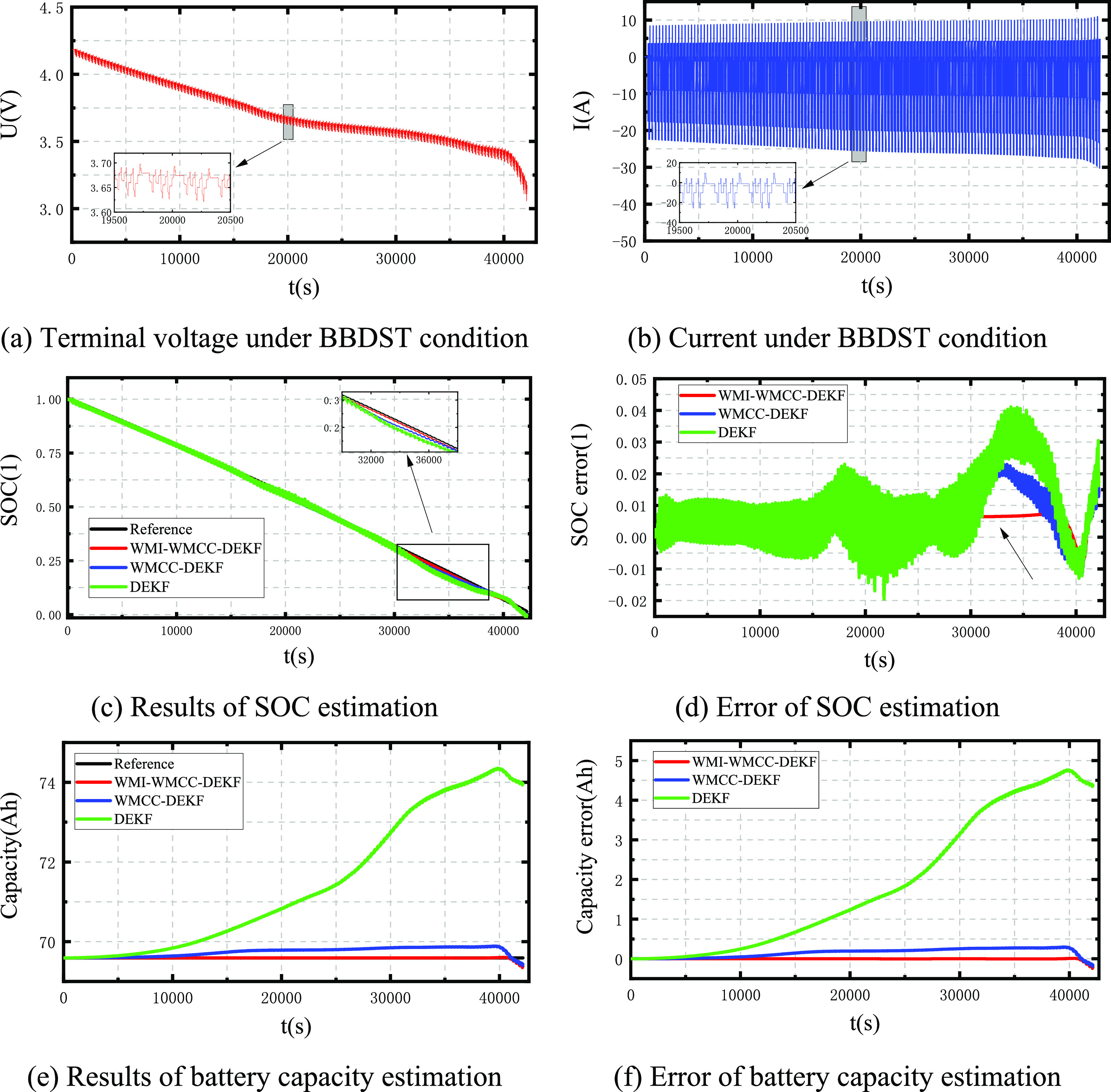
4.6. Test the Target Algorithm Using BBDST Working Condition Data with Mixed Gaussian Noise

The BBDST working condition formed by the collection of the real operation data of Beijing bus includes the driving conditions such as starting, acceleration, braking, and taxiing, which can be a more realistic simulation of the power battery facing the work scene, can further verify the performance of the target algorithm. In order to test the performance of the three algorithms under BBDST conditions, the data used also include BBDST data without additional noise, BBDST data with weak mixed Gaussian noise, and BBDST data with strong mixed Gaussian noise. The final test results are shown in Figure 3–5, respectively, and the performance statistics of SOC and capacity are shown in Tables 3 and4.

Table 3. Performance Indicators of Three Algorithms for SOC Estimation Using BBDST Working Condition Data with Different Types of Noise.

	no added noise		noise1		noise2
HPPC	MAE	RMSE	MAE	RMSE	MAE	RMSE
DEKF	0.0411	0.0132	0.2126	0.0775	0.5516	0.1735
WMCC–DEKF	0.0268	0.0096	0.0277	0.0093	0.0328	0.0097
WMI-WMCC–DEKF	0.0267	0.0058	0.0268	0.0056	0.0290	0.0059

Table 4. Performance Indicators of Three Algorithms for Capacity Estimation Using BBDST Working Condition Data with Different Types of Noise (the Unit of MAE and RMSE Is Ah).

	no added noise		noise1		noise2
HPPC	MAE	RMSE	MAE	RMSE	MAE	RMSE
DEKF	4.7637	2.5075	5.1372	2.6270	5.3329	2.3111
WMCC–DEKF	0.2987	0.1870	0.3093	0.1891	0.3595	0.2202
WMI-WMCC–DEKF	0.2419	0.0204	0.2418	0.0201	0.2823	0.0205

4.6.1. Performance of Target Algorithm in Processing Data without Additional Noise

Similar to the HPPC condition test, first verify the performance of three algorithms WMI-WMCC–DEKF, WMCC–DEKF, and DEKF under BBDST wording condition without additional noise (the terminal voltage is shown in Figure 13a, and the current is shown in Figure 13b), and the results are shown in Figure 13c–f. It can be concluded from Figure 13c that all three algorithms can achieve the estimation of SOC, but from the local zoom map indicated by the arrow, the WMI-WMCC–DEKF algorithm is superior to the other two algorithms, which can also be seen from Figure 13d on the SOC estimation error. In Figure 13d, it can be seen from the arrow that the estimation error of the WMI-WMCC–DEKF algorithm for SOC is much smaller than that of the WMCC–DEKF algorithm and the DEKF algorithm, and the error fluctuation range of the WMI-WMCC–DEKF algorithm is small, indicating that the algorithm has good dynamic adaptability and anti-interference ability. When the three algorithms are in the low SOC region (<10%), due to the strong nonlinear relationship between SOC and U_OC, and the influence of polynomial fitting coefficient and order, the errors of the three algorithms at this time have great changes. In Table 3, the specific indexes of SOC estimation performance show that the MAE and RMSE values of the WMI-WMCC–DEKF algorithm are 0.0267 and 0.0058, respectively, while the MAE and RMSE values of the WMCC–DEKF are 0.0268 and 0.0096. MAE and RMSE values of the DEKF algorithm are 0.0411 and 0.0132, respectively. Compared with the WMCC–DEKF algorithm, the WMI-WMCC–DEKF algorithm decreases by 0.4 and 41.7%, respectively, and compared with the DEKF algorithm, the WMI-WMCC–DEKF algorithm decreases by 35 and 56.1%, respectively. For the estimation of battery capacity, it can be seen from Figure 13e,f that the estimation accuracy of the WMI-WMCC–DEKF algorithm is much higher than that of the other two algorithms, and its estimated value is almost the same as the actual value (except for the low SOC area). It can be seen from Table 4 that in the statistical indicators of capacity estimation results, the MAE and RMSE values of the WMI-WMCC–DEKF algorithm are 19 and 89.1% lower than those of the WMCC–DEKF algorithm, and 94.9 and 99.2% lower than those of the DEKF algorithm. Based on the above analysis, it can be seen that the WMI-WMCC–DEKF algorithm has the best performance under BBDST working conditions without additional noise. The co-estimation performance of the three algorithms for SOC and capacity meets the following relation: WMI-WMCC–DEKF > WMCC–DEKF > DEKF.

Figure 13.

Results of co-estimation of SOC and capacity by three algorithms using BBDST working condition data without additional noise.

4.6.2. Performance of Target Algorithm in Processing Data with Weak Gaussian Mixture Noise

When weak mixed Gaussian noise is added to the BBDST working condition data (as shown in Figure 14b), the estimation results of SOC and capacity of the three algorithms are shown in Figure 14c–f. From Figure 14c, it can be clearly concluded that after working for some time, the estimation results of the DEKF algorithm begin to be inaccurate and cannot work normally, which indicates that the DEKF algorithm has poor anti-noise interference ability, while the WMI-WMCC–DEKF and the WMCC–DEKF can work normally, so the following analysis only focuses on these two algorithms. In Figure 14d, it can be concluded that the SOC estimated error value of the WMI-WMCC–DEKF algorithm is much smaller than that of the WMCC–DEKF algorithm, and the fluctuation range of the error value is small, which shows that the WMI-WMCC–DEKF has better anti-noise performance and dynamic adaptation performance. For specific quantitative indicators, it can be concluded from Table 3 that the MAE and RMSE values of the WMI-WMCC–DEKF algorithm are 0.0268 and 0.0056, respectively, while the MAE and RMSE values of the WMCC–DEKF algorithm are 0.0277 and 0.0093, respectively. The former algorithm is 3.2 and 39.8% lower than the latter algorithm. In the capacity estimation, it can be found from Figure 14e,f that the capacity estimation accuracy of the WMI-WMCC–DEKF algorithm is much higher than that of the WMCC–DEKF algorithm. However, at the dotted line pointed by the arrow in the paper, both algorithms have large errors in capacity estimation, which is mainly due to the fact that the battery is in a low SOC region, and the increase of the degree of electrochemical reaction in this region and the nonlinearity between SOV-U_OC have a great impact on the estimation error of the algorithm. It can be seen from Table 4 that in capacity estimation, MAE and RMSE of the WMI-WMCC–DEKF algorithm are reduced by 21.8 and 89.4%, respectively, compared with the WMCC–DEKF algorithm. From the above analysis, we can see that the WMI-WMCC–DEKF algorithm shows good anti-noise performance in the weak mixed Gaussian noise scene and can achieve an accurate estimation of SOC and capacity.

Figure 14.

Results of co-estimation of SOC and capacity by three algorithms using BBDST working condition data with weak mixed Gaussian noise.

4.6.3. Performance of Target Algorithm in Processing Data with Strong Gaussian Mixture Noise

When strong Gaussian mixture noise is added to the BBDST data (As shown in Figure 15b), the estimation of SOC and battery capacity by the three algorithms is shown in Figure 15c–f. It can be concluded from Figure 15c that the WMI-WMCC–DEKF algorithm and the WMCC–DEKF algorithm can realize the estimation of SOC, while the DEKF algorithm does not work properly, which indicates that the DEKF algorithm does not have anti-noise ability under strong Gaussian mixed noise. Therefore, we only analyze the performance of the WMI-WMCC–DEKF and the WMCC–DEKF algorithms. It can be seen from Figure 15d that the WMI-WMCC–DEKF algorithm has a smaller SOC estimation error and smaller error fluctuation than the WMCC–DEKF algorithm, which indicates that the WMI-WMCC–DEKF algorithm has better anti-noise performance and dynamic adaptive performance. As can be seen from Table 3, the MAE and RMSE of the WMI-WMCC–DEKF algorithm are 0.0290 and 0.0059, respectively, which are 11.6 and 39.2% lower than MAE (0.0328) and RMSE (0.0097) of the WMCC–DEKF algorithm. In the estimation of capacity, the estimation accuracy of the WMI-WMCC–DEKF algorithm is much higher than that of the WMCC–DEKF algorithm, which can be seen in Figure 15e,f. At the dotted line pointed by the arrow, the two algorithms are affected by the low SOC area, and their estimation error is increased. For the specific indicators of capacity estimation, the MAE and RMSE values of the WMI-WMCC–DEKF algorithm are 0.2823 and 0.0205, respectively, which are 21.5 and 90.7% lower than the MAE (0.3595) and RMSE (0.2202) values of the WMCC–DEKF algorithm. According to the above analysis, under strong mixed Gaussian noise, the WMI-WMCC–DEKF algorithm shows good anti-interference ability and can achieve accurate estimation of SOC and capacity.

Figure 15.

Results of co-estimation of SOC and capacity by three algorithms using BBDST working condition data with strong mixed Gaussian noise.

4.7. Test the Target Algorithm Using Data with Outlier Noise

To more visually evaluate the performance of the co-estimation of SOC and battery capacity by the three algorithms when the collected power battery data has outliers, the outliers as shown in Figure 9 are added to the HPPC and BBDST data, respectively (as shown in Figures 16b and 17b). The estimation results of the three algorithms are shown in Figures 16c–f and 17c–f, and the performance statistics are shown in Tables 5 and 6. It can be seen from Figure 16c and Table 5 that the estimated value of SOC of the DEKF algorithm will be far more than that of the other two algorithms when there are outliers in the data, which indicates that the DEKF algorithm has the extremely weak anti-outlier ability. Therefore, only the WMI-WMCC–DEKF and WMCC–DEKF algorithms are analyzed in the subsequent performance analysis. It can be seen from the arrow point in Figure 16d that the SOC estimated error of the WMI-WMCC–DEKF algorithm at outliers is much smaller than that of the WMCC–DEKF algorithm. Besides, except for individual values in the tail, the SOC estimated error of the WMI-WMCC–DEKF algorithm has a very small fluctuation range. This shows that the algorithm can eliminate the influence of outlier noise and obtain good estimation performance. In Table 5, the MAE and RMSE values of the WMI-WMCC–DEKF algorithm are 0.0411 and 0.0015, respectively, which are 67.8 and 85.3% lower than the MAE (0.1275) and RMSE (0.0102) values of the WMCC–DEKF algorithm. In capacity estimation, it can be seen from Figure 16e,f that, except for the tail individual value pointed by the arrow, the capacity estimation error of the WMI-WMCC–DEKF algorithm is far less than that of the WMCC–DEKF algorithm. As can be seen from Table 6, the MAE and RMSE values of the WMI-WMCC–DEKF algorithm are 58.8 and 94.3% lower than those of the WMCC–DEKF algorithm, respectively.

Figure 16.

Results of co-estimation of SOC and capacity by three algorithms using HPPC working condition data with outlier noise.

Figure 17.

Results of co-estimation of SOC and capacity by three algorithms using BBDST working condition data with outlier noise.

Table 5. Performance Indicators of Three Algorithms for SOC Estimation Using HPPC Working Condition and BBDST Working Condition Data with Added Outliers.

	HPPC		BBDST
SOC	MAE	RMSE	MAE	RMSE
DEKF	1.1301	0.1360	1.3400	0.1272
WMCC–DEKF	0.1275	0.0102	0.0268	0.0097
WMI-WMCC–DEKF	0.0411	0.0015	0.0267	0.0059

Table 6. Performance Indicators of Three Algorithms for Capacity Estimation Using HPPC Working Condition and BBDST Working Condition Data with Added Outliers (the Unit of MAE and RMSE Is Ah).

	HPPC		BBDST
capacity	MAE	RMSE	MAE	RMSE
DEKF	0.1938	0.1398	4.9304	2.6465
WMCC–DEKF	0.1385	0.0124	0.2862	0.1768
WMI-WMCC–DEKF	0.0570	7.1026 × 10–4	0.2418	0.0204

The outlier data is added to the BBDST working condition data that is closer to the real-use environment of the power battery. The results of the three algorithms for the co-estimation of battery SOC and capacity using this data are shown in Figure 17. In Figure 17c, it can be seen that the DEKF algorithm has a large estimation error in the place where the outlier data exists (the arrow point), and the estimation error of the other two algorithms is much smaller than that of DEKF algorithm, indicating that DEKF algorithm is sensitive to non-Gaussian outlier noise and is highly susceptible to interference. Therefore, only the performance of WMI-WMCC–DEKF and WMCC–DEKF algorithms is quantified. It can be concluded from Figure 17d that, first, the SOC estimation error of the WMI-WMCC–DEKF algorithm at the outlier data indicated by the arrow is far less than the SOC estimation error of the WMCC–DEKF algorithm, which shows that the WMI-WMCC–DEKF algorithm has a stronger ability to resist outlier interference; Second, in the whole SOC estimation process, the fluctuation range of the SOC estimation error of the WMI-WMCC–DEKF algorithm is smaller than that of the WMCC–DEKF algorithm, which shows that the WMI-WMCC–DEKF algorithm has better dynamic adaptability and stability; Third, in the low SOC region, both algorithms have large error values, which indicates that in the low SOC region, the internal electrochemical reaction of the battery and the error of the fitting function will have a great impact on both algorithms. In terms of specific quantitative indicators, it can be seen from Table 5 that the MAE and RMSE of the WMI-WMCC–DEKF algorithm are, respectively, 0.4 and 39.2% lower than those of the WMCC–DEKF algorithm. In the capacity estimation, we can find from Figure 17e,f that on the left side of the imaginary line segment pointed by the arrow, the capacity estimation error of the WMI-WMCC–DEKF algorithm is far less than the capacity estimation error of the WMCC–DEKF algorithm. However, large estimation errors appear on the right side of the dotted line, which is mainly affected by the large estimation errors of the two algorithms in the low SOC interval. For specific quantitative indicators, we can see from Table 6 that the MAE and RMSE values of the WMI-WMCC–DEKF algorithm are 0.2418 and 0.0204, respectively, which are 15.5 and 88.5% lower than the MAE (0.2862) and RMSE (0.1768) of the WMCC–DEKF algorithm, respectively.

5. Results and Discussion

The test results of the three algorithms using HPPC and BBDST working conditions data with different noise types show that: (1) the three algorithms can process the operating conditions without additional noise and can achieve co-estimation of battery SOC and capacity, but the overall performance meets the relationship of WMI-WMCC–DEKF > WMCC–DEKF > DEK. (2) When the weak mixed Gaussian noise or strong mixed Gaussian noise is added, the DEKF algorithm cannot continue to work normally, while the WMI-WMCC–DEKF algorithm and the WMCC–DEKF algorithm can complete the estimation of the battery SOC and capacity, which shows that the algorithm based on the maximum correlation entropy criterion has better anti-noise performance than the algorithm based on the least squares criterion. (3) The WMI-WMCC–DEKF algorithm has better anti-noise performance and dynamic adaptability than the WMCC–DEKF algorithm. In the process of outlier noise testing for the three algorithms, the DEKF algorithm is very sensitive to outliers and will produce a great estimation error at the outlier noise compared with the other two algorithms. Compared with the WMCC–DEKF algorithm, the WMI-WMCC–DEKF algorithm has a much smaller estimation error at outlier noise, which shows a very superior ability to eliminate outlier noise. Therefore, from the whole test, it can be concluded that the WMI-WMCC–DEKF algorithm proposed in this paper has good adaptability to non-Gaussian noise, and shows superior battery SOC and capacity estimation capabilities.

6. Conclusions

In the traditional co-estimation of battery SOC and capacity, most algorithms mainly consider the influence of Gaussian noise, but lithium-ion batteries are likely to be affected by non-Gaussian noise (such as outliers) due to the complex operating environment. To solve this problem, different from the traditional minimum mean square error criterion, this paper proposes to use the maximum correlation entropy criterion to design the estimation algorithm. First, the parameter estimation algorithms based on the least squares error criterion and the maximum correlation entropy criterion are given, respectively, and the basic steps of the parameter identification algorithm are given in combination with the second-order Thevenin model used in this paper. Then, the WMCC-EKF algorithm is derived based on the maximum correlation entropy criterion. By adding the weighted multi-innovation calculation unit to the closed-loop control loop corresponding to the algorithm, the extended Kalman filtering algorithm based on the weighted multi-innovation and weighted maximum entropy criterion is proposed. Then, on the basis of the proposed WMI-WMCC-EKF algorithm, the WMI-WMCC–DEKF algorithm is proposed for the co-estimation of battery SOC and capacity. Finally, to verify the performance of the target algorithm, this paper presents three noise generation models: weak Gaussian mixed noise generation model, strong Gaussian mixed noise generation model, and outlier noise generation model. The three algorithms of DEKF, WMCC–DEKF, and WMI-WMCC–DEKF are tested and analyzed in HPPC and BBDST working condition data containing the above three kinds of noises. The experimental results show that: (1) WMI-WMCC–DEKF and WMCC–DEKF algorithms based on the maximum correlation entropy criterion can also work in the Gaussian noise environment, and the performance is better than the DEKF algorithm based on the minimum mean square error criterion. (2) The performance of WMCC–DEKF and MCC–DEKF algorithms based on the maximum correlation entropy criterion is much better than that of DEKF algorithm based on the minimum mean square error criterion against the above three kinds of noises. However, the DEKF algorithm is particularly sensitive to mixed noises and is difficult to work normally. (3) In the whole testing process, the performance of the WMI-WMMC–DEKF algorithm is much better than that of the WMCC–DEKF algorithm. The above experimental results fully show that the proposed WMI-WMCC–DEKF algorithm has an excellent performance in complex noise environments.

The authors declare no competing financial interest.

References

- Zou R.; Duan Y.; Wang Y.; Pang J.; Liu F.; Sheikh S. R. A Novel Convolutional Informer Network for Deterministic and Probabilistic State-of-Charge Estimation of Lithium-Ion Batteries. J. Energy Storage 2023, 57, 106298 10.1016/j.est.2022.106298. [DOI] [Google Scholar]
- Park J.; Kim K.; Park S.; Baek J.; Kim J. Complementary Cooperative SOC/Capacity Estimator Based on the Discrete Variational Derivative Combined with the DEKF for Electric Power Applications. Energy 2021, 232, 121023 10.1016/j.energy.2021.121023. [DOI] [Google Scholar]
- Duan J.; Wang P.; Ma W.; Qiu X.; Tian X.; Fang S. State of Charge Estimation of Lithium Battery Based on Improved Correntropy Extended Kalman Filter. Energies 2020, 13, 4197. 10.3390/en13164197. [DOI] [Google Scholar]
- Xiao D.; Fang G.; Liu S.; Yuan S.; Ahmed R.; Habibi S.; Emadi A. Reduced-Coupling Coestimation of SOC and SOH for Lithium-Ion Batteries Based on Convex Optimization. IEEE Trans. Power Electron. 2020, 35, 12332–12346. 10.1109/TPEL.2020.2984248. [DOI] [Google Scholar]
- Chen Z.; Shen W.; Chen L.; Wang S. Adaptive Online Capacity Prediction Based on Transfer Learning for Fast Charging Lithium-Ion Batteries. Energy 2022, 248, 123537 10.1016/j.energy.2022.123537. [DOI] [Google Scholar]
- Shu X.; Li G.; Shen J.; Yan W.; Chen Z.; Liu Y. An Adaptive Fusion Estimation Algorithm for State of Charge of Lithium-Ion Batteries Considering Wide Operating Temperature and Degradation. J. Power Sources 2020, 462, 228132 10.1016/j.jpowsour.2020.228132. [DOI] [Google Scholar]
- Shrivastava P.; Soon T.; Bin Idris M.; Mekhilef S.; Adnan S. Combined State of Charge and State of Energy Estimation of Lithium-Ion Battery Using Dual Forgetting Factor-Based Adaptive Extended Kalman Filter for Electric Vehicle Applications. IEEE Trans. Veh. Technol. 2021, 70, 1200–1215. 10.1109/TVT.2021.3051655. [DOI] [Google Scholar]
- Ouyang T.; Xu P.; Chen J.; Lu J.; Chen N. An Online Prediction of Capacity and Remaining Useful Life of Lithium-Ion Batteries Based on Simultaneous Input and State Estimation Algorithm. IEEE Trans. Power Electron. 2021, 36, 8102–8113. 10.1109/TPEL.2020.3044725. [DOI] [Google Scholar]
- Shu X.; Li G.; Shen J.; Lei Z.; Chen Z.; Liu Y. An Adaptive Multi-State Estimation Algorithm for Lithium-Ion Batteries Incorporating Temperature Compensation. Energy 2020, 207, 118262 10.1016/j.energy.2020.118262. [DOI] [Google Scholar]
- Bian X.; Wei Z.; He J.; Yan F.; Liu L. A Two-Step Parameter Optimization Method for Low-Order Model-Based State-of-Charge Estimation. IEEE Trans. Transp. Electrific. 2021, 7, 399–409. 10.1109/TTE.2020.3032737. [DOI] [Google Scholar]
- Li X.; Wang Z.; Zhang L. Co-Estimation of Capacity and State-of-Charge for Lithium-Ion Batteries in Electric Vehicles. Energy 2019, 174, 33–44. 10.1016/j.energy.2019.02.147. [DOI] [Google Scholar]
- Wang L.; Ma J.; Zhao X.; Li X.; Zhang K.; Jiao Z. Adaptive Robust Unscented Kalman Filter-Based State-of-Charge Estimation for Lithium-Ion Batteries with Multi-Parameter Updating. Electrochim. Acta 2022, 426, 140760 10.1016/j.electacta.2022.140760. [DOI] [Google Scholar]
- Shrivastava P.; Soon T. K.; Idris M. Y. I. B.; Mekhilef S. Overview of Model-Based Online State-of-Charge Estimation Using Kalman Filter Family for Lithium-Ion Batteries. Renewable Sustainable Energy Rev. 2019, 113, 109233 10.1016/j.rser.2019.06.040. [DOI] [Google Scholar]
- Zhang Z.; Jiang L.; Zhang L.; Huang C. State-of-Charge Estimation of Lithium-Ion Battery Pack by Using an Adaptive Extended Kalman Filter for Electric Vehicles. J. Energy Storage 2021, 37, 102457 10.1016/j.est.2021.102457. [DOI] [Google Scholar]
- Xiong R.; Cao J.; Yu Q.; He H.; Sun F. Critical Review on the Battery State of Charge Estimation Methods for Electric Vehicles. IEEE Access 2018, 6, 1832–1843. 10.1109/ACCESS.2017.2780258. [DOI] [Google Scholar]
- Sun D.; Yu X.; Wang C.; Zhang C.; Huang R.; Zhou Q.; Amietszajew T.; Bhagat R. State of Charge Estimation for Lithium-Ion Battery Based on an Intelligent Adaptive Extended Kalman Filter with Improved Noise Estimator. Energy 2021, 214, 119025. 10.1016/j.energy.2020.119025. [DOI] [Google Scholar]
- Wu M.; Qin L.; Wu G.; Huang Y.; Shi C. State of Charge Estimation of Power Lithium-Ion Battery Based on a Variable Forgetting Factor Adaptive Kalman Filter. J. Energy Storage 2021, 41, 102841 10.1016/j.est.2021.102841. [DOI] [Google Scholar]
- He Z.; Li Y.; Sun Y.; Zhao S.; Lin C.; Pan C.; Wang L. State-of-Charge Estimation of Lithium Ion Batteries Based on Adaptive Iterative Extended Kalman Filter. J. Energy Storage 2021, 39, 102593 10.1016/j.est.2021.102593. [DOI] [Google Scholar]
- He Z.; Yang Z.; Cui X.; Li E. A Method of State-of-Charge Estimation for EV Power Lithium-Ion Battery Using a Novel Adaptive Extended Kalman Filter. IEEE Trans. Veh. Technol. 2020, 69, 14618–14630. 10.1109/TVT.2020.3032201. [DOI] [Google Scholar]
- Li J.; Ye M.; Gao K.; Xu X.; Wei M.; Jiao S. Joint Estimation of State of Charge and State of Health for Lithium-Ion Battery Based on Dual Adaptive Extended Kalman Filter. Int. J. Energy Res. 2021, 45, 13307–13322. 10.1002/er.6658. [DOI] [Google Scholar]
- Peng N.; Zhang S.; Guo X.; Zhang X. Online Parameters Identification and State of Charge Estimation for Lithium-ion Batteries Using Improved Adaptive Dual Unscented Kalman Filter. Int. J. Energy Res. 2021, 45, 975–990. 10.1002/er.6088. [DOI] [Google Scholar]
- Fan T.-E.; Liu S.-M.; Tang X.; Qu B. Simultaneously Estimating Two Battery States by Combining a Long Short-Term Memory Network with an Adaptive Unscented Kalman Filter. J. Energy Storage 2022, 50, 104553 10.1016/j.est.2022.104553. [DOI] [Google Scholar]
- Peng J.; Luo J.; He H.; Lu B. An Improved State of Charge Estimation Method Based on Cubature Kalman Filter for Lithium-Ion Batteries. Appl. Energy 2019, 253, 113520 10.1016/j.apenergy.2019.113520. [DOI] [Google Scholar]
- Liu Z.; Dang X.; Jing B.; Ji J. A Novel Model-Based State of Charge Estimation for Lithium-Ion Battery Using Adaptive Robust Iterative Cubature Kalman Filter. Electr. Power Sys. Res. 2019, 177, 105951 10.1016/j.epsr.2019.105951. [DOI] [Google Scholar]
- Linghu J.; Kang L.; Liu M.; Luo X.; Feng Y.; Lu C. Estimation for State-of-Charge of Lithium-Ion Battery Based on an Adaptive High-Degree Cubature Kalman Filter. Energy 2019, 189, 116204 10.1016/j.energy.2019.116204. [DOI] [Google Scholar]
- Chen Z.; Sun H.; Dong G.; Wei J.; Wu J. Particle Filter-Based State-of-Charge Estimation and Remaining-Dischargeable-Time Prediction Method for Lithium-Ion Batteries. J. Power Sources 2019, 414, 158–166. 10.1016/j.jpowsour.2019.01.012. [DOI] [Google Scholar]
- Deng Z.; Hu X.; Lin X.; Che Y.; Xu L.; Guo W. Data-Driven State of Charge Estimation for Lithium-Ion Battery Packs Based on Gaussian Process Regression. Energy 2020, 205, 118000 10.1016/j.energy.2020.118000. [DOI] [Google Scholar]
- Hossain Lipu M. S.; Hannan M. A.; Hussain A.; Ayob A.; Saad M. H. M.; Karim T. F.; How D. N. T. Data-Driven State of Charge Estimation of Lithium-Ion Batteries: Algorithms, Implementation Factors, Limitations and Future Trends. J. Cleaner Prod. 2020, 277, 124110 10.1016/j.jclepro.2020.124110. [DOI] [Google Scholar]
- Chen C.; Xiong R.; Yang R.; Shen W.; Sun F. State-of-Charge Estimation of Lithium-Ion Battery Using an Improved Neural Network Model and Extended Kalman Filter. J. Cleaner Prod. 2019, 234, 1153–1164. 10.1016/j.jclepro.2019.06.273. [DOI] [Google Scholar]
- Zhang G.; Xia B.; Wang J.; Ye B.; Chen Y.; Yu Z.; Li Y. Intelligent State of Charge Estimation of Battery Pack Based on Particle Swarm Optimization Algorithm Improved Radical Basis Function Neural Network. J. Energy Storage 2022, 50, 104211 10.1016/j.est.2022.104211. [DOI] [Google Scholar]
- Lipu M. S. H.; Hannan M. A.; Hussain A.; Saad M. H. M.; Ayob A.; Uddin M. N.. Extreme Learning Machine for SOC Estimation of Lithium-Ion Battery Using Gravitational Search Algorithm. In 2018 IEEE Industry Applications Society Annual Meeting (IAS); IEEE: Portland, OR, 2018; pp 1–8.
- Cui D.; Xia B.; Zhang R.; Sun Z.; Lao Z.; Wang W.; Sun W.; Lai Y.; Wang M. A Novel Intelligent Method for the State of Charge Estimation of Lithium-Ion Batteries Using a Discrete Wavelet Transform-Based Wavelet Neural Network. Energies 2018, 11, 995. 10.3390/en11040995. [DOI] [Google Scholar]
- Hossain Lipu M. S.; Hannan M. A.; Hussain A.; Ayob A.; Saad M. H. M.; Muttaqi K. M. State of Charge Estimation in Lithium-Ion Batteries: A Neural Network Optimization Approach. Electronics 2020, 9, 1546. 10.3390/electronics9091546. [DOI] [Google Scholar]
- Chemali E.; Kollmeyer P. J.; Preindl M.; Emadi A. State-of-Charge Estimation of Li-Ion Batteries Using Deep Neural Networks: A Machine Learning Approach. J. Power Sources 2018, 400, 242–255. 10.1016/j.jpowsour.2018.06.104. [DOI] [Google Scholar]
- Xuan L.; Qian L.; Chen J.; Bai X.; Wu B. State-of-Charge Prediction of Battery Management System Based on Principal Component Analysis and Improved Support Vector Machine for Regression. IEEE Access 2020, 8, 164693–164704. 10.1109/ACCESS.2020.3021745. [DOI] [Google Scholar]
- Bian C.; He H.; Yang S. Stacked Bidirectional Long Short-Term Memory Networks for State-of-Charge Estimation of Lithium-Ion Batteries. Energy 2020, 191, 116538 10.1016/j.energy.2019.116538. [DOI] [Google Scholar]
- Ren X.; Liu S.; Yu X.; Dong X. A Method for State-of-Charge Estimation of Lithium-Ion Batteries Based on PSO-LSTM. Energy 2021, 234, 121236 10.1016/j.energy.2021.121236. [DOI] [Google Scholar]
- Stroe D.-I.; Swierczynski M.; Kar S. K.; Teodorescu R. Degradation Behavior of Lithium-Ion Batteries During Calendar Ageing-The Case of the Internal Resistance Increase. IEEE Trans. Ind. Appl. 2018, 54, 517–525. 10.1109/TIA.2017.2756026. [DOI] [Google Scholar]
- Yang D.; Wang Y.; Pan R.; Chen R.; Chen Z. State-of-Health Estimation for the Lithium-Ion Battery Based on Support Vector Regression. Appl. Energy 2018, 227, 273–283. 10.1016/j.apenergy.2017.08.096. [DOI] [Google Scholar]
- Stroe D.; Swierczynski M.; Stroe A.; Kaer S. K.; Teodorescu R. Lithium-ion Battery Power Degradation Modelling by Electrochemical Impedance Spectroscopy. IET Renewable Power Generation 2017, 11, 1136–1141. 10.1049/iet-rpg.2016.0958. [DOI] [Google Scholar]
- Liu D.; Yin X.; Song Y.; Liu W.; Peng Y. An On-Line State of Health Estimation of Lithium-Ion Battery Using Unscented Particle Filter. IEEE Access 2018, 6, 40990–41001. 10.1109/ACCESS.2018.2854224. [DOI] [Google Scholar]
- Sui X.; He S.; Vilsen S. B.; Meng J.; Teodorescu R.; Stroe D.-I. A Review of Non-Probabilistic Machine Learning-Based State of Health Estimation Techniques for Lithium-Ion Battery. Applied Energy 2021, 300, 117346 10.1016/j.apenergy.2021.117346. [DOI] [Google Scholar]
- Ge M.-F.; Liu Y.; Jiang X.; Liu J. A Review on State of Health Estimations and Remaining Useful Life Prognostics of Lithium-Ion Batteries. Measurement 2021, 174, 109057 10.1016/j.measurement.2021.109057. [DOI] [Google Scholar]
- Dai H.; Zhao G.; Lin M.; Wu J.; Zheng G. A Novel Estimation Method for the State of Health of Lithium-Ion Battery Using Prior Knowledge-Based Neural Network and Markov Chain. IEEE Trans. Ind. Electron. 2019, 66, 7706–7716. 10.1109/TIE.2018.2880703. [DOI] [Google Scholar]
- Zhang S.; Zhai B.; Guo X.; Wang K.; Peng N.; Zhang X. Synchronous Estimation of State of Health and Remaining Useful Lifetime for Lithium-Ion Battery Using the Incremental Capacity and Artificial Neural Networks. J. Energy Storage 2019, 26, 100951 10.1016/j.est.2019.100951. [DOI] [Google Scholar]
- Chen Z.; Sun M.; Shu X.; Xiao R.; Shen J. Online State of Health Estimation for Lithium-Ion Batteries Based on Support Vector Machine. Appl. Sci. 2018, 8, 925. 10.3390/app8060925. [DOI] [Google Scholar]
- Feng X.; Weng C.; He X.; Han X.; Lu L.; Ren D.; Ouyang M. Online State-of-Health Estimation for Li-Ion Battery Using Partial Charging Segment Based on Support Vector Machine. IEEE Trans. Veh. Technol. 2019, 68, 8583–8592. 10.1109/TVT.2019.2927120. [DOI] [Google Scholar]
- Yang D.; Zhang X.; Pan R.; Wang Y.; Chen Z. A Novel Gaussian Process Regression Model for State-of-Health Estimation of Lithium-Ion Battery Using Charging Curve. J. Power Sources 2018, 384, 387–395. 10.1016/j.jpowsour.2018.03.015. [DOI] [Google Scholar]
- Song Y.; Liu D.; Liao H.; Peng Y. A Hybrid Statistical Data-Driven Method for on-Line Joint State Estimation of Lithium-Ion Batteries. Appl. Eerergy 2020, 261, 114408 10.1016/j.apenergy.2019.114408. [DOI] [Google Scholar]
- Sun X.; Zhong K.; Han M. A Hybrid Prognostic Strategy with Unscented Particle Filter and Optimized Multiple Kernel Relevance Vector Machine for Lithium-Ion Battery. Measurement 2021, 170, 108679 10.1016/j.measurement.2020.108679. [DOI] [Google Scholar]
- Chen Z.; Xue Q.; Xiao R.; Liu Y.; Shen J. State of Health Estimation for Lithium-Ion Batteries Based on Fusion of Autoregressive Moving Average Model and Elman Neural Network. IEEE Access 2019, 7, 102662–102678. 10.1109/ACCESS.2019.2930680. [DOI] [Google Scholar]
- Shen P.; Ouyang M.; Lu L.; Li J.; Feng X. The Co-Estimation of State of Charge, State of Health, and State of Function for Lithium-Ion Batteries in Electric Vehicles. IEEE Trans. Veh. Technol. 2018, 67, 92–103. 10.1109/TVT.2017.2751613. [DOI] [Google Scholar]
- Shuzhi Z.; Xu G.; Xiongwen Z. A Novel One-Way Transmitted Co-Estimation Framework for Capacity and State-of-Charge of Lithium-Ion Battery Based on Double Adaptive Extended Kalman Filters. J. Energy Storage 2021, 33, 102093 10.1016/j.est.2020.102093. [DOI] [Google Scholar]
- Song Z.; Hou J.; Li X.; Wu X.; Hu X.; Hofmann H.; Sun J. The Sequential Algorithm for Combined State of Charge and State of Health Estimation of Lithium-Ion Battery Based on Active Current Injection. Energy 2020, 193, 116732 10.1016/j.energy.2019.116732. [DOI] [Google Scholar]
- Zhang S.; Zhang X. A Multi Time-Scale Framework for State-of-Charge and Capacity Estimation of Lithium-Ion Battery under Optimal Operating Temperature Range. J. Energy Storage 2021, 35, 102325 10.1016/j.est.2021.102325. [DOI] [Google Scholar]
- Jiang C.; Wang S.; Wu B.; Fernandez C.; Xiong X.; Coffie-Ken J. A State-of-Charge Estimation Method of the Power Lithium-Ion Battery in Complex Conditions Based on Adaptive Square Root Extended Kalman Filter. Energy 2021, 219, 119603 10.1016/j.energy.2020.119603. [DOI] [Google Scholar]
- Yang B.; Cao L.; Ran D.; Xiao B. Centered Error Entropy Kalman Filter with Application to Satellite Attitude Determination. Trans. Inst. Meas. Control. 2021, 43, 3055–3070. 10.1177/01423312211019867. [DOI] [Google Scholar]
- Jwo D.-J.; Lai J.-H. Minimum Error Entropy Based EKF for GPS Code Tracking Loop. Comput. Mater. Continua 2021, 67, 2883–2898. 10.32604/cmc.2021.015102. [DOI] [Google Scholar]
- Wang G.; Xue R.; Wang J. A Distributed Maximum Correntropy Kalman Filter. Signal Processing 2019, 160, 247–251. 10.1016/j.sigpro.2019.02.030. [DOI] [Google Scholar]
- Liu X.; Qu H.; Zhao J.; Chen B.. Extended Kalman Filter under Maximum Correntropy Criterion2016. In 2016 International Joint Conference on Neural Networks (IJCNN); IEEE: Vancouver, BC, Canada, 2016; pp 1733–1737.
- Ma F.; Liu F.; Zhang X.; Wang P.; Bai H.; Guo H. An Ultrasonic Positioning Algorithm Based on Maximum Correntropy Criterion Extended Kalman Filter Weighted Centroid. SIViP 2018, 12, 1207–1215. 10.1007/s11760-018-1272-2. [DOI] [Google Scholar]
- Wang W.; Tse C. K.; Wang S. Generalized Correntropy Sparse Gauss–Hermite Quadrature Filter for Epidemic Tracking on Complex Networks. IEEE Trans. Syst. Man Cybern, Syst. 2022, 52, 2770–2778. 10.1109/TSMC.2021.3052538. [DOI] [Google Scholar]
- A D Massignan J.; B A London J. Jr.; Miranda V. Tracking Power System State Evolution with Maximum-Correntropy-Based Extended Kalman Filter. J. Modern Power Syst. Clean Energy 2020, 8, 616–626. 10.35833/MPCE.2020.000122. [DOI] [Google Scholar]
- Liu X.; Ren Z.; Lyu H.; Jiang Z.; Ren P.; Chen B. Linear and Nonlinear Regression-Based Maximum Correntropy Extended Kalman Filtering. IEEE Trans. Syst. Man Cybern, Syst. 2021, 51, 3093–3102. 10.1109/TSMC.2019.2917712. [DOI] [Google Scholar]
- Kulikova M. V. Square-Root Algorithms for Maximum Correntropy Estimation of Linear Discrete-Time Systems in Presence of Non-Gaussian Noise. Syst. Control Lett. 2017, 108, 8–15. 10.1016/j.sysconle.2017.07.016. [DOI] [Google Scholar]
- Izanloo R.; Fakoorian S. A.; Yazdi H. S.; Simon D.. Kalman Filtering Based on the Maximum Correntropy Criterion in the Presence of Non-Gaussian Noise2016. In 2016 Annual Conference on Information Science and Systems (CISS); IEEE: Princeton, NJ, USA, 2016; pp 500–505.
- Maletić F.; Hrgetić M.; Deur J. Dual Nonlinear Kalman Filter-Based SoC and Remaining Capacity Estimation for an Electric Scooter Li-NMC Battery Pack. Energies 2020, 13, 540. 10.3390/en13030540. [DOI] [Google Scholar]