Predicting reprogramming-related gene expression from cell morphology in human induced pluripotent stem cells

Abstract

Purification is essential before differentiating human induced pluripotent stem cells (hiPSCs) into cells that fully express particular differentiation marker genes. High-quality iPSC clones are typically purified through gene expression profiling or visual inspection of the cell morphology; however, the relationship between the two methods remains unclear. We investigated the relationship between gene expression levels and morphology by analyzing live-cell, phase-contrast images and mRNA profiles collected during the purification process. We employed these data and an unsupervised image feature extraction method to build a model that predicts gene expression levels from morphology. As a benchmark, it was confirmed that the method can predict the gene expression levels from tissue images for cancer genes, performing as well as state-of-the-art methods. We then applied the method to iPSCs and identified two genes that are well predicted from cell morphology. Although strong batch (or possibly donor) effects resulting from the reprogramming process preclude the ability to use the same model to predict across batches, prediction within a reprogramming batch is sufficiently robust to provide a practical approach for estimating expression levels of a few genes and monitoring the purification process.

INTRODUCTION

Human induced pluripotent stem cells (hiPSCs) are of growing importance in both basic and translational biomedical research due to their capacity to differentiate into any cell type and proliferate indefinitely. HiPSCs are derived from easily accessible somatic cells, like leukocytes or skin fibroblasts, using different iPSC reprogramming methods (Buganim et al., 2013; Malik and Rao, 2013). Unfortunately, currently available iPSC reprogramming methods are stochastic, which leaves a subset of cells partially reprogrammed and with low pluripotency. Therefore, generating high-quality iPSCs requires an extensive and time-consuming purification process to eliminate partially reprogrammed cells (Brown et al., 2010; Mack et al., 2011).

During the purification process iPSC clones with high pluripotency and stemness are selected based on either gene expression profiling data, such as RNA-seq, or cell morphology as evaluated by visual inspection or image analysis (Marx et al., 2013; Maddah et al., 2014; Tokunaga et al., 2014; Kato et al., 2016; Hoshikawa et al., 2019; Doulgkeroglou et al., 2020; Piotrowski et al., 2021). Historically, gene expression profiling has been used as a primary cell quality indicator to improve protocols (Brown et al., 2010; González et al., 2011; Mack et al., 2011; Wakao et al., 2012; Teshigawara et al., 2017), whereas visual inspection or image analysis is used to monitor daily cell quality (Marx et al., 2013; Maddah et al., 2014; Tokunaga et al., 2014; Kato et al., 2016; Hoshikawa et al., 2019; Doulgkeroglou et al., 2020; Piotrowski et al., 2021). However, because of major limitations of these approaches, another evaluation method should be explored to make the purification process more efficient in the future. For example, although gene expression profiling gives a direct readout of stemness and differentiation markers useful for improving iPSC culture protocols (Brown et al., 2010; Mack et al., 2011; D’Antonio et al., 2017; Sekine et al., 2020), the method is destructive, precluding further analysis of the cell. Therefore, the outcome can be estimated only through statistical interpretation using multiple samples, which are costly to grow and propagate. On the other hand, morphological analysis of cell images is nondestructive, with a qualitative relationship between cell quality and morphology as evidenced by the success of iPSCs to date (Wakao et al., 2012; Healy and Ruban, 2014; Tokunaga et al., 2014; Kato et al., 2016; Wakui et al., 2017); however, this method identifies iPSCs with high pluripotency based on their morphology such as compact shape with less cytoplasm (Healy and Ruban, 2014; Wakui et al., 2017), thus using indirect readouts prone to errors and misinterpretation, with no clear link to underlying gene expression. Therefore, an improved quality evaluation method for identifying high-quality iPSC populations that overcomes limitations of the current methodologies by bridging gene expression with morphology in a nondestructive manner would help address this major bottleneck in the iPSC generation process.

Very recently, several studies have demonstrated that morphological features can be used to predict gene expression in various contexts (Cutiongco et al., 2020; He et al., 2020; Schmauch et al., 2020; Dawood et al., 2021; Haghighi et al., 2022). For example, supervised deep learning models, such as a convolutional neural network (CNN), were trained with data sets of pathological images and spatial gene expression profiles obtained by single-cell sequencing of the exact same sample to predict cancer gene expression from pathological images (He et al., 2020). The resulting models were able to accurately link morphology with gene expression, suggesting that a similar strategy could be extended beyond cancer and applied to the iPSC purification process. However, these strategies require expensive single-cell sequencing measurements, which limits their widespread adoption.

In this study, to overcome existing limitations and provide the community with a more robust, affordable, easy to implement evaluation method useful for more efficient iPSC purification, we developed a method to predict the expression of iPSC genes from bright-field cell morphology during the iPSC purification process. Our method was designed to use multiple label-free, phase-contrast images of cells growing in culture vessels and bulk-level gene expression profiles of these cells, measured for each vessel. Thus, unlike most previous studies, the gene expression profiles (by virtue of being at the bulk level) do not have a one-to-one correspondence with individual cells. Therefore, we employed an approach based on an unsupervised deep learning model to extract morphology features from each image and then created a simple support vector regression (SVR) model to predict gene expression based on the image features of each vessel. We validate our approach on a benchmark data set, as well as data from iPSC samples obtained from experimental conditions designed to simulate the iPSC purification process.

RESULTS

Gene expression data set assembly for predictive model building

To build a robust predictive model, we focused our initial efforts on acquiring high-quality imaging and bulk gene expression data under conditions that simulate the iPSC purification process. We generated six data sets composed of 29 iPSC clones derived from peripheral blood mononuclear cells (PBMCs) of 15 donors. Data sets A1–A3 were obtained by culturing 15 iPSC clones derived from a single donor, and data sets B1–B3 were generated by culturing 14 iPSC clones derived from 14 different donors (Supplemental Table S1). To simulate different stages of iPSC purification processes, all iPSCs were cultured for three passages with increasingly sized vessels (six-well plate, T75 flask, and T150 flasks) for each passage respectively (Supplemental Figure S1). In every passage, the cells were passaged on day 4, and phase-contrast imaging and gene expression measurements were performed before passaging.

Our gene expression analysis was done using targeted amplicon sequencing, a bulk RNA-seq strategy focused on a subset of genes. We measured expression levels for 980 genes related to stemness and pluripotency. We filtered the 980 genes by their average (mean) and coefficient of variation values (CV) across all the samples to identify genes with sufficient expression levels and significant variance, as those suggest predictive power needed for robust model building. The final list contained 218 genes, including three Yamanaka factor genes: KLF4, SOX2, and POU5F1 (Figure 1). Thus, these data represent the input gene expression data for our predictive model training.

FIGURE 1:

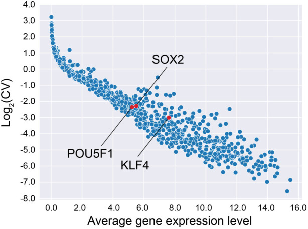
Distribution of gene expression levels and variation across samples. Each dot represents a gene expression of a single gene. After filtering based on the average (X-axis) and CV (Y-axis) of the gene expression level, we retained 218 genes out of the 980 genes (top right quadrant), including three genes of particular interest (red dots).

Image-based gene expression prediction pipeline

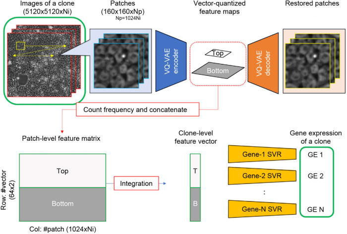
To develop a robust image-based gene expression prediction pipeline that would require a limited amount of bulk-level mRNA data, we adopted a two-stage approach (Figure 2). First, given the number of samples (87; 29 clones at three different time points), we treated each individual iPSC phase-contrast image as a collection of thousands of pieces of imaging information by splitting it into patches of 160 × 160 pixels (72 μm), resulting in 1024 patches per image, to suit the memory constraints of subsequent deep learning model training. To extract features from these patches, we used a modified VQ-VAE-2 model (Razavi et al., 2019) as a self-supervised feature extraction method (Supplemental Figure S4). The variation of the cell quality inside a patch is negligible and can be represented by a latent vector of the VQ-VAE-2 model. Thus, in stage 1, we extracted vector-quantized feature maps by applying the trained VQ-VAE-2 model to all the patches (see Materials and Methods for details). Next, in stage 2, we used this feature extraction process together with SVR to obtain 128-dimensional feature vectors for each image patch, which were then averaged to produce a single 128-dimensional profile for each sample. Vector quantization inherent in the VQ-VAE-2 model enables easy preservation of the feature distribution in a sample, whereas alternatives require statistical calculation, which may lead to loss of the feature distribution information, in order to integrate the features of the patches into a single profile.

FIGURE 2:

Gene expression prediction pipeline. We split iPSC phase-contrast images of a sample into patches of 160 × 160 pixels (72 μm) each, extracted feature maps using the VQ-VAE encoder, and integrated the maps into a feature vector. We constructed 218 SVR models corresponding to the 218 target genes. Np: Number of patches, Ni: Number of images.

VQ-VAE-2 model validation

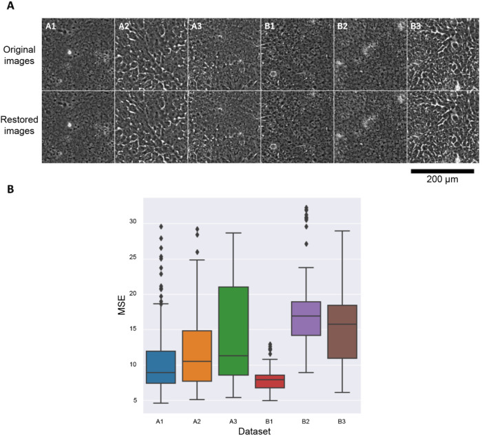
To confirm that the trained VQ-VAE-2 model extracted sufficient image features to reconstruct images, we evaluated the reconstruction accuracy for each data set using mean-squared error (MSE) between the original images and the reconstructed images (Figure 3). We used data set A3 for the VQ-VAE-2 model training. Then, we randomly sampled 10 images (10,240 patches) of each data set to calculate the MSE. All of the MSEs are lower than 36, which means that the average pixel-wise error for the eight-bit images (256 levels) is less than 6 (2.3%) for all images; little difference in the images was found by visual inspection across the data sets (Figure 3A). We thus concluded that our VQ-VAE-2 model was sufficiently trained, as it can extract the image features essential to reliably reconstruct the iPSC images.

FIGURE 3:

Image restoration accuracy of each data set. The VQ-VAE-2 model was trained on a single data set (A3) and applied to all data sets to extract image features. (A) Comparison of the original images and the restored images by the model trained with data set A3. (B) Average MSEs calculated between the original images and the restored images (lower MSE is better). All MSEs were less than 36 (i.e., averages were less than 6) for eight-bit images, indicating good restoration performance regardless of the data set.

Extracted image features relate to experimentally defined quality categories

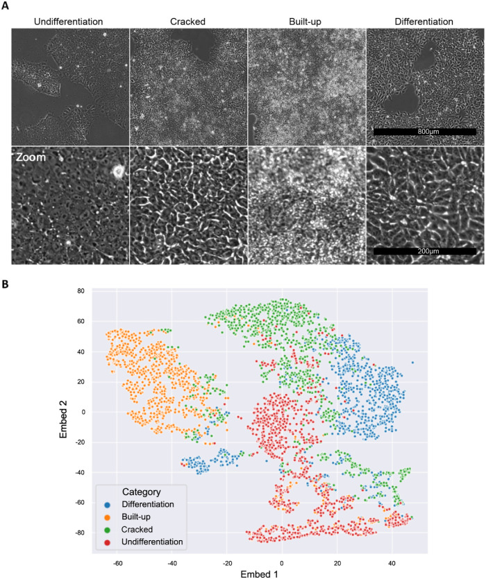
To examine whether the VQ-VAE-2 model adequately extracted the meaningful image features related to biology, we investigated the relationship between the image features and the four morphological categories (undifferentiation, cracked, built-up, and differentiation) that are routinely used by iPSC culture experts to identify undifferentiated “good” cells (Healy and Ruban, 2014; Wakui et al., 2017). As mentioned in the Introduction, these categories have no clear link to underlying gene expression, but they likely contain some information that is useful for predicting gene expression levels. We selected a representative image (5120 × 5120 pixels) for each category from data set A3 and obtained 1024 image patches (160 × 160 pixels) for each of the categories (Figure 4A). Then, the patches were processed by the trained VQ-VAE-2 model to extract the image features, yielding 1024 image feature vectors in total. We visualized the distribution of the extracted image feature vectors for each category by t-SNE dimension reduction (Figure 4B). In addition to that unsupervised analysis, we evaluated the classification accuracy of the quality categories based on the extracted image feature vectors by a support vector machine (SVM) model (Table 1). The image feature vectors were split 3:1 for training and test, respectively. We obtained 89.3% test accuracy for the quality categories, after optimizing hyperparameters by threefold cross-validation for gamma and C with RBF kernel. Taken together, this analysis provides additional validation of our image features as accurate representations of iPSC quality and an excellent agreement between the VQ-VAE-2 model and expert curation.

FIGURE 4:

iPSC quality categories defined by the culture experts. (A) Typical morphology of each category. Four morphological categories are visually defined by iPSC culture experts. Undifferentiation: Good iPSCs with high stemness and pluripotency. Cells have little cytoplasm and prominent nucleoli. Cracked: Upper-middle quality. Cells still have a morphology similar to that of undifferentiated cells, but some kind of differentiation-related activity appears as cracks. Built-up: Lower-middle quality. Cells are crowded, stacking on top of each other, and cell morphology cannot be observed at all. Differentiation: Low quality. Totally differentiated and not useful for the subsequent differentiation process. Cells of this category have a flat, dark, and large appearance compared with the cells of the other categories. (B) t-SNE plot based on the image features extracted by the VQ-VAE-2 model trained with the A3 data set. Each color represents images of the quality categories defined by the experts, which mostly exist in different regions in the feature space despite this being an unsupervised analysis, which does not involve any training with expert annotations.

TABLE 1:

Classification performance for the quality categories based on the image features.

Hierarchical clustering of gene expression levels and image features

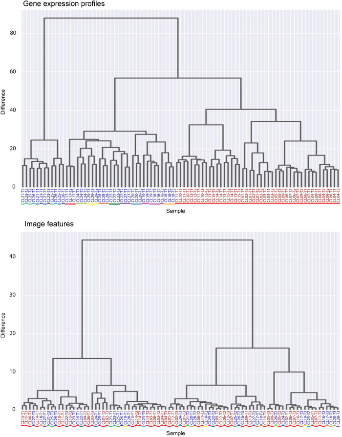
To see the variance of the gene expression profiles across data sets, we performed hierarchical clustering analysis. We found that the gene expression profiles consisting of 218 genes have different characteristics between experiment A (one donor) and experiment B (14 donors) (Figure 5, top), also showing that the different samples derived from the same donor (#CL1-15 of experiment A and #CL16 of experiment B) were classified into the different clusters. We also performed hierarchical clustering of the image features across the data sets. This analysis revealed that image features of experiment A and experiment B do not display clear clustering (Figure 5, bottom). This suggests that batch (or possibly donor) effects and their impact on gene expression profiles may pose a significant challenge to developing a single predictive model that would accurately fit all the data sets and that multiple models may be needed.

FIGURE 5:

Hierarchical clustering results for the gene expression profiles (top) and the image features (bottom) across all 87 samples. The color of each sample name represents the experiment. Samples in blue: experiment A (clone #CL1-15). Samples in red: experiment B (clone #CL16-29). The color of each bar under sample names represents a different donor. Clones #1-15 of experiment A and #16 of experiment B are derived from the same donor. Image features do not show a clear difference between experiment A and experiment B, while gene expression profiles form distinct clusters between experiments.

Validation with public benchmark data set shows performance equivalent to that of an end-to-end approach

Before testing the VQ-VAE–based approach on the gene expression-from-bright-field-iPSC-images prediction task, we tested it on a distinct but related task—predicting gene expression using histopathologic images from a public spatial transcriptomics breast cancer data set (He et al., 2020). This data set contains 30,612 spots with gene expression profiles in 68 breast tissue sections from 23 patients with breast cancer. The sections were scanned at 20× magnification, and 26,949 distinct mRNA expression levels were measured in spots with a diameter of 100 µm arranged in a grid with a center-to-center distance of 200 µm. We compared the prediction performances of our model and the end-to-end CNN model DenseNet-121 (Huang et al., 2017), which was previously used on this data set, by focusing on the expression of the 250 genes with the highest mean expression for all the spots (Validation Methodology in Supplement S1). The final prediction performance for each gene represents a median value of 23 correlation coefficients between measured gene expressions and predicted gene expressions for each patient’s single cells, obtained by leave-one-out cross-validation of 23 patients. As shown in Table 2, three of the top five genes were consistent (p = 3.8e-5, Fisher’s exact test) and our model performed comparably to the end-to-end CNN model (He et al., 2020) (Validation Methodology in Supplement S1). These results gave us confidence that our method can predict gene expression from images with accuracy comparable to that of the current state-of-the-art but without needing labels to learn image representations.

TABLE 2:

Validation results on a published benchmark.

	DenseNet	Ours
1	*HSP90AB1(0.325)	*FASN(0.390)
2	*FASN(0.324)	DDX5(0.372)
3	*GNAS(0.319)	*HSP90AB1(0.343)
4	ACTG1(0.317)	TPT1(0.314)
5	FN1(0.315)	*GNAS(0.309)

Genes with top five prediction performances. Values in parentheses are the median of correlation coefficients between measured and predicted gene expressions obtained by leave-one-out cross-validation of 23 patients. Common genes are marked with an asterisk. Three of the top five predicted genes matched those of ST-Net.

Prediction of gene expression based on iPSC data sets

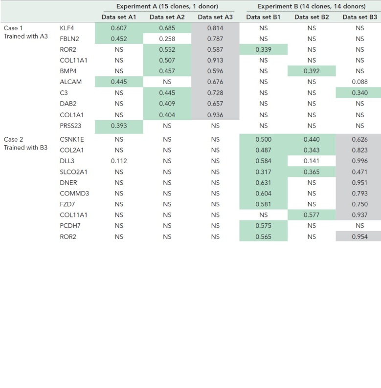
Having demonstrated the efficacy of the method on a benchmark task, we employed our method to predict gene expression values from extracted image features of iPSCs. We evaluated the prediction performance for all iPSC data sets using SVR models trained with either data set A3 (one donor, time point 3) or B3 (14 donors, time point 3) (Table 3). In both cases, threefold cross-validation within the training data set was performed to optimize SVR model hyperparameters for each gene as described in Materials and Methods. We then calculated the coefficient of determination (R²) and corresponding significance corrected by the Benjamini–Hochberg method (false discovery rate [FDR]) between the predicted gene expression and the measured gene expression for every data set. Then, we picked the top 10 genes with the highest R² value and that passed significance of α = 0.05.

TABLE 3: .

Prediction performance for the top 10 genes across experiments.

Cells with R²>0.3 between predicted and measured gene expression levels are highlighted in green. NS: not significant with FDR correction (α = 0.05). Results for the training set are highlighted in light gray.

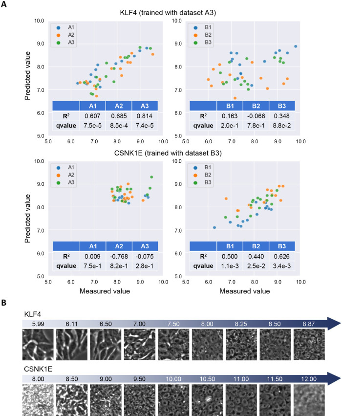
When trained on the single-donor data set (A3, time point 3), the best-predicted gene was KLF4. For KLF4 (Figure 6A, top), the model obtained good predictions on the data sets A1 and A2 with R² = 0.607 and 0.685 (and A3 used for training = 0.834) but did not perform well on the data sets of experiment B. This indicates that training does not generalize well across the experiments either due to technical variation (batch effects) or due to the differing donors. For the other genes, the model had R² > 0.3 for only one or two data sets other than the data set used for model training.

FIGURE 6:

Gene prediction results. (A) Prediction accuracy on each data set for KLF4 and CSNK1E. Predicted (y-axis) vs. measured (x-axis) expression levels (log2) for KLF4 and CSNK1E using the trained models as labeled. (B) Cell morphology and predicted gene expression levels for KLF4 and CSNK1E. The numbers represent the predicted gene expression levels corresponding to each image. The patches are collected from the data sets of experiments A and B for KLF4 and CSNK1E, respectively.

We wondered whether training on a larger set of donors might improve predictions. We therefore trained on the 14-donor data set (B3, time point 3) and found that the best-predicted gene was CSNK1E. For CSNK1E (Figure 6A, bottom), predictions were good in data sets B1 and B2 with R² = 0.500 and 0.440, again demonstrating good generalizability across time points within a batch. This model did not perform well on experiment A data sets, however, which indicates that training on many donors does not improve generalization across the experimental batches. To investigate how specific morphological characteristics correspond to best-predicted gene expression levels, we selected patch images from the data sets that were particularly high- or low-expressing for the best-predicted gene for each batch. We observed that the cells show differentiation-like morphology when the predicted expression level of KLF4 is low and undifferentiation-like (“good”) morphology as the predicted KLF4 expression level increases for images within experiment A (Figure 6B). For images within experiment B, we also confirmed that as the predicted CSNK1E expression increases, the cells change their appearance from built-up–like morphology to undifferentiated-like morphology, until they become larger and the cell boundaries become unclear (Figure 6B). Taken together, although batch- or donor-specific variations impact prediction performance, morphological analysis suggests that changes in image features correlate with changes in predicted expression levels for the best-predicted genes.

DISCUSSION

In this study, we developed an evaluation strategy that provides information useful for improving the iPSC purification process by using cell morphology captured by phase-contrast microscopy. To achieve this, we introduced a new method to predict gene expression levels based on label-free images of cells that employs a regression model trained on image features extracted using an unsupervised deep learning model, VQ-VAE-2. This method enables the nondestructive evaluation of cell quality through prediction of gene expression levels, which can lead to further improvements in iPSC culture protocols in the future, unlike conventional evaluation strategies that rely on destructive gene expression measurements such as RNA-seq or morphology-based methods that are nondestructive but difficult to relate to differentiation markers.

We benchmarked the performance of our method using a completely different setup—a public data set of tissue slide images and spatial gene expression data—and demonstrated a result similar to that of the state-of-the-art. We also investigated the relationship between the image features captured by our method and the iPSC morphological quality categories experimentally defined by the iPSC culture experts (Healy and Ruban, 2014; D’Antonio et al., 2017; Wakui et al., 2017). The results showed that there is a correspondence between the morphological quality categories and the image features extracted from unstained phase-contrast images, allowing morphological quality categories to be predicted from the image features with 89.3% accuracy. It is difficult to examine the relationship effectively with a limited number of samples between gene expression and the quality categories because our bulk-level gene expression data set lacks spatial information. However, because there exists a relationship between image features and categories, as well as between gene expression and image features, our results suggest that the method we developed could also assist in linking image features with both gene expression and the quality categories. This would further facilitate visual inspection and iPSC purification and make the process more reliable.

When we employed our approach to predict gene expression from image features, we identified two top-predicted genes, KLF4 and CSNK1E, from two different experiments. For KLF4, we observed that as the predicted expression increases, the appearance of cells changes from differentiated-like to undifferentiated-like. This observation agrees with the known biology of KLF4, as it has previously been established that KLF4 is a key gene for iPSC reprogramming and dedifferentiation process in somatic cells and that this process can be paused by manipulating the KLF4 expression (Nishimura et al., 2014; Bialkowska et al., 2017). For CSNK1E, we observed that as the predicted expression increases, the cellular morphology changes from built-up–like, to flat, undifferentiated-like, to having an unclear cell boundary, indicating that the cells were progressively dissociating. This observation appears to be consistent with CSNK1E biology as this protein accelerates cell migration and cell dissociation (Simpson et al., 2008; Bar et al., 2018). Therefore, the gene expression predictions from image features for top genes are in good agreement with their established biological functions.

Our results also highlight that we obtained two significantly different predictions in two different experiments, experiment A, which included 15 clones from the same patient, and experiment B, which included samples from 14 different patients. This suggests that batch (or possibly donor) effects, that is, nonbiological factors in an experiment that are observable in the data and known to pose a major challenge in high-dimensional biology (Goh et al., 2017), play a significant role in our work as well. We observed that the predictive model works well only when the training and test data set are from the same batch (i.e., the same experiment); training a model on many donors (experiment B) did not dramatically improve predictions versus training on a single donor. We also observed that the list of genes with the best R² values is different across the batches. This suggests that not only are the models nongeneralizable across the batches but also the relationships between morphology and gene expression appear to be different across the two batches. This discrepancy is consistent with the observation from our hierarchical clustering analysis, where we noted that strong batch (or possibly donor) effects are observed in gene expression data but not in the imaging data.

In our experience, batch effects are predominantly due to the stochastic nature of the iPSC reprogramming process itself (Hanna et al., 2009; Teshigawara et al., 2017). In fact, the iPSCs for the two experiments (A and B) were reprogrammed separately, so it is very likely that the batch effects are indeed driven by the reprogramming process, although we could not eliminate the possibility of the donor effects using our data set. Given this source of batch effects, our overall approach can be used to make predictions of expression levels only within a reprogramming batch. Despite this current caveat, our methodology might be usefully implemented by collecting gene expression data and training a model early in the iPSC reprogramming process and applying it to future time points of the batch, thus eliminating repeated gene expression profiling for the many subsequent rounds of cloning. For instance, a prediction model might be trained on a specific batch in the reprogramming process to be stored in a cell bank, then the model might be used to monitor cell quality for the cells taken out from the same bank.

The method might also be used in studies that aim to identify better culture protocols that yield cells having desired expression levels for specific genes. Using images instead of mRNA is nondestructive and additionally allows monitoring the spatial distribution of gene expression within a culture. This could allow adjusting the culture protocol more precisely based on the spatial information of gene expression, replacing the current methodology to develop culture protocols using bulk gene expression measurements. Furthermore, batch-effect correction techniques applied to such data, together with a more diverse set of training data, may further improve the ability to generalize the models, reduce the need for gene expression profiling, and enable automated reprogramming processes based on live-cell imaging.

In conclusion, we explored the relationship between iPSC morphology and gene expression within iPSC multi-clone data sets collected during the iPSC purification process. We used phase-contrast images as a morphology readout and bulk RNA-seq as gene expression data and trained the models to use image features to predict gene expression. Although batch (or possibly donor) effects, driven by the iPSC reprogramming process, limit our ability to generalize the model across reprogramming batches, the proposed approach may allow stem cell facilities to automatically track the iPSC purification process using phase-contrast imaging alone.

MATERIALS AND METHODS

Request a protocol through Bio-protocol.

Data acquisition

In this study, we used six data sets composed of 29 iPSCs clones derived from peripheral blood mononuclear cells (PBMCs) of 15 donors. The culture of iPSCs was carried out in two phases. We first cultured 15 iPSC clones (experiment A) all derived from a single donor and then cultured 14 iPSCs clones derived from 14 donors (experiment B), which includes the same one donor used in experiment A, one clone per donor, using the same iPSC culture protocol (Mack et al., 2011). To simulate the iPSC purification process, all iPSCs were cultured for three passages with different types of vessels, six-well plate, T75 flask, and T150 flasks for each passage, respectively (Supplemental Figure S1). T150 flasks will continue to be used for a while thereafter in the actual purification process. In every passage, the cells were passaged on day 4, and phase-contrast imaging and gene expression measurements were performed before passaging. As a result of these culture experiments, we obtained six data sets composed of 29 clones and three time points (87 samples, Supplemental Table S1).

Phase-contrast imaging

The images were obtained by a phase-contrast microscope (Nikon Ti2-E) with a 10× objective lens (Nikon Plan Fluor 10×/0.30 DL) and a 25 megapixel camera (25CXP1; CIS). We captured single-focal-plane grayscale images of cells for each culture vessel. We captured 60, 100, and 100 images for time point 1, time point 2, and time point 3, respectively. The resolution and the dimensions of each image are 0.45 µm/pixel and 5120 × 5120 pixels, respectively.

Gene expression normalization method

To enable comparison of the expression levels between samples, measured expression profiles were normalized by the total number of reads for each sample. Then, we took a logarithm of base 2 after adding a pseudo count of 1 to prevent zeros.

VQ-VAE-2 model training

We trained a VQ-VAE-2 model as it is, with K of 64 and D of 64 on the images of a single data set using the Adam optimizer (Kingma and Ba, 2014) with a learning rate of 1e-4 to minimize MSE between the input patch and the restored patch. Specifically, we utilized the A3 data set for training as it generally provides a wider range of morphological variation in cells cultured in larger vessels at time point 3 compared with time points 1 and 2. To prepare the A3 data set for model training, we split all included images into small 160 × 160 pixel patches. The model was trained for 50 epochs with a batch size of 32 using the PyTorch machine learning framework.

Extraction of image feature vectors

We extracted the latent feature vector of a sample by the following procedure. First, we split all the images of a sample into small patches. Image size is 5120 × 5120 pixels, and we adopted a patch size of 160 × 160 pixels, so the number of patches per image is 1024. Each patch contains roughly 30 cells. Second, we extracted vector-quantized feature maps by applying the trained VQ-VAE-2 model to all the patches. Here we have two feature maps with different resolutions (20 and 40 pixels each) per patch. Third, we counted the appearance frequencies of each embedding vector from the feature maps for all the patches. We totaled these and normalized the total frequency of embedding vectors by each resolution after adding a pseudo count of 1 to prevent zeros from being used in the next step and then computed the logarithm of base 2 to get the sample’s profile.

Gene expression prediction model training

We applied SVR to predict the gene expression of each sample from sample-level image features using the scikit-learn machine learning library in Python. Training of SVR models and optimization of the model hyperparameters were done for each gene; in other words, we constructed as many SVR models as target genes (n = 218). For SVR models, the linear kernel function was adopted, and hyperparameters (C, epsilon) were searched from the following lists by a grid-search algorithm with threefold cross-validation in the training data set:

• C: [1,2,3, …,100]

• epsilon: [0, 0.05, 0.10, …, 0.50]

Hierarchical clustering

Hierarchical clustering was performed using the linkage function of the Scipy library. The Ward method was used to calculate distances. For images, clustering was performed on the image features of each sample. For gene expression, clustering was performed for the expression profiles of the extracted 218 genes after normalization.

Morphology feature association study

Gene prediction was performed for 10 representative images selected from each sample. The VQ-VAE-2 model trained with the images of a single data set (A3) was applied to all patches of the selected images to obtain image features for each patch. Then the SVR models to predict genes were applied to the image features. Each SVR model was applied only to the image features calculated from the data set that the model was trained with. The KLF4 prediction model was applied to the image features obtained from the data set of experiment A. The CSNK1E prediction model was applied to the image features obtained from the data set of experiment B. To obtain gene expression levels patch-wisely, the feature averaging step was omitted.

Data and code availability

We used the VQ-VAE-2 implementation from https://github.com/rosinality/vq-vae-2-pytorch and did not make any modifications. All the relevant parameters for model training and feature extraction are documented above.

Abbreviations used:

FDR

false discovery rate

hiPSC

human induced pluripotent stem cell

MSE

mean squared error

PBMC

peripheral blood mononuclear cell

SVM

support vector machine

SVR

support vector regression

t-SNE

t-distributed stochastic neighbor embedding

VQ-VAE2

vector quantized variable auto encoder 2

REFERENCES

- Bar I, Merhi A, Larbanoix L, Constant M, Haussy S, Laurent S, Canon J, Delrée P (2018). Silencing of casein kinase 1 delta reduces migration and metastasis of triple negative breast cancer cells. Oncotarget 9, 30821. [DOI] [PMC free article] [PubMed] [Google Scholar]
- Bialkowska AB, Yang VW, Mallipattu SK (2017). Krüppel-like factors in mammalian stem cells and development. Development 144, 737–754. [DOI] [PMC free article] [PubMed] [Google Scholar]
- Brown ME, Rondon E, Rajesh D, Mack A, Lewis R, Feng X, Zitur L, Learish RD, Nuwaysir EF (2010). Derivation of induced pluripotent stem cells from human peripheral blood T lymphocytes. PLoS One 5, e11373. [DOI] [PMC free article] [PubMed] [Google Scholar]
- Buganim Y, Faddah DA, Jaenisch R (2013). Mechanisms and models of somatic cell reprogramming. Nat Rev Genet 14, 427–439. [DOI] [PMC free article] [PubMed] [Google Scholar]
- Cutiongco MF, Jensen BS, Reynolds PM, Gadegaard N (2020). Predicting gene expression using morphological cell responses to nanotopography. Nat Commun 11, 1–13. [DOI] [PMC free article] [PubMed] [Google Scholar]
- D’Antonio M, Woodruff G, Nathanson JL, D’Antonio-Chronowska A, Arias A, Matsui H, Williams R, Herrera C, Reyna SM, Yeo GW, et al. (2017). High-throughput and cost-effective characterization of induced pluripotent stem cells. Stem Cell Rep 8, 1101–1111. [DOI] [PMC free article] [PubMed] [Google Scholar]
- Dawood M, Branson K, Rajpoot NM, Minhas F (2021). All you need is color: image based spatial gene expression prediction using neural stain learning. ArXiv abs/2108.10446, 2021. [Google Scholar]
- Doulgkeroglou MN, Nubila AD, Niessing B, König N, Schmitt RH, Damen J, Szilvassy SJ, Chang W, Csontos L, Louis S, et al. (2020). Automation, monitoring, and standardization of cell product manufacturing. Front Bioeng Biotechnol 8, 811. [DOI] [PMC free article] [PubMed] [Google Scholar]
- Goh WWB, Wang W, Wong L (2017). Why batch effects matter in omics data, and how to avoid them. Trends Biotechnol 35, 498–507. [DOI] [PubMed] [Google Scholar]
- González F, Boué S, Belmonte J (2011). Methods for making induced pluripotent stem cells: reprogramming à la carte. Nat Rev Genet 12, 231–242. [DOI] [PubMed] [Google Scholar]
- Haghighi M, Caicedo JC, Carpenter AE, Singh S (2022). High-dimensional gene expression and morphology profiles of cells across 28,000 genetic and chemical perturbations. Nat Methods 19, 1550–1557. [DOI] [PMC free article] [PubMed] [Google Scholar]
- Hanna JSaha KPando BZon JVLengner CJCreyghton MPOudenaarden AVJaenisch R (2009). Direct cell reprogramming is a stochastic process amenable to acceleration. Nature 462, 595–601. [DOI] [PMC free article] [PubMed] [Google Scholar]
- He BBergenstråhle LStenbeck LAbid AAndersson ABorg AMaaskola JLundeberg JZou J (2020). Integrating spatial gene expression and breast tumour morphology via deep learning. Nat Biomed Eng 4, 827–834. [DOI] [PubMed] [Google Scholar]
- Healy L, Ruban L (2014). Atlas of Human Pluripotent Stem Cells in Culture, New York, NY: Springer. [Google Scholar]
- Hoshikawa E, Sato T, Kimori Y, Suzuki A, Haga K, Kato H, Tabeta K, Nanba D, Izumi K (2019). Noninvasive measurement of cell/colony motion using image analysis methods to evaluate the proliferative capacity of oral keratinocytes as a tool for quality control in regenerative medicine. J Tissue Eng 10, 2041731419881528. [DOI] [PMC free article] [PubMed] [Google Scholar]
- Huang G, Liu Z, Van Der Maaten L, Weinberger KQ (2017). Densely connected convolutional networks. In: Proceedings of the IEEE Conference on Computer Vision and Pattern Recognition, 4700–4708.
- Kato R, Matsumoto M, Sasaki H, Joto R, Okada M, Ikeda Y, Kanie K, Suga M, Kinehara M, Yanagihara K, et al. (2016). Parametric analysis of colony morphology of non-labelled live human pluripotent stem cells for cell quality control. Sci Rep 6, 1–12. [DOI] [PMC free article] [PubMed] [Google Scholar]
- Kingma DP, Ba J (2014). Adam: a method for stochastic optimization. arXiv:1412.6980.
- Mack AA, Kroboth S, Rajesh D, Wang WB (2011). Generation of induced pluripotent stem cells from CD34+ cells across blood drawn from multiple donors with non-integrating episomal vectors. PLoS One 6, e27956. [DOI] [PMC free article] [PubMed] [Google Scholar]
- Maddah M, Shoukat-Mumtaz U, Nassirpour S, Loewke K (2014). A system for automated, noninvasive, morphology-based evaluation of induced pluripotent stem cell cultures. J Lab Autom 19, 454–460. [DOI] [PubMed] [Google Scholar]
- Malik N, Rao MS (2013). A review of the methods for human iPSC derivation. In: Pluripotent Stem Cells, ed. Lakshmipathy U, Vemuri M., Methods in Molecular Biology, Vol. 997, Totowa, NJ: Humana Press, 23–33. [DOI] [PMC free article] [PubMed] [Google Scholar]
- Marx U, Schenk F, Behrens J, Meyr U, Wanek P, Zang W, Schmitt R, Brüstle O, Zenke M, Klocke F (2013). Automatic production of induced pluripotent stem cells. Procedia CIRP 5, 2–6. [Google Scholar]
- Nishimura K, Kato T, Chen C, Oinam L, Shiomitsu E, Ayakawa D, Ohtaka M, Fukuda A, Nakanishi M, Hisatake K (2014). Manipulation of KLF4 expression generates iPSCs paused at successive stages of reprogramming. Stem Cell Rep 3, 915–929. [DOI] [PMC free article] [PubMed] [Google Scholar]
- Piotrowski T, Rippel O, Elanzew A, Nießing B, Stucken S, Jung S, König N, Haupt S, Stappert L, Brüstle O, et al. (2021). Deep-learning-based multi-class segmentation for automated, non-invasive routine assessment of human pluripotent stem cell culture status. Comput Biol Med 129, 104172. [DOI] [PubMed] [Google Scholar]
- Razavi A, van den Oord A, Vinyals O (2019). Generating diverse high-fidelity images with vq-vae-2. Advances in neural information processing systems, Cambridge, UK: The MIT Press, Vol 32, 14866–14876. [Google Scholar]
- Schmauch B, Romagnoni A, Pronier E, Saillard C, Maillé P, Calderaro J, Kamoun A, Sefta M, Toldo S, Zaslavskiy M, et al. (2020). A deep learning model to predict RNA-Seq expression of tumours from whole slide images. Nat Commun 11, 1–15. [DOI] [PMC free article] [PubMed] [Google Scholar]
- Sekine K, Tsuzuki S, Yasui R, Kobayashi T, Ikeda K, Hamada Y, Kanai E, Camp JG, Treutlein B, Ueno Y, et al. (2020). Robust detection of undifferentiated iPSC among differentiated cells. Sci Rep 10, 1–9. [DOI] [PMC free article] [PubMed] [Google Scholar]
- Simpson KJ, Selfors LM, Bui J, Reynolds A, Leake D, Khvorova A, Brugge JS (2008). Identification of genes that regulate epithelial cell migration using an siRNA screening approach. Nat Cell Biol 10, 1027–1038. [DOI] [PubMed] [Google Scholar]
- Teshigawara R, Cho J, Kameda M, Tada T (2017). Mechanism of human somatic reprogramming to iPS cell. Lab Invest 97, 1152–1157. [DOI] [PubMed] [Google Scholar]
- Tokunaga K, Saitoh N, Goldberg IG, Sakamoto C, Yasuda Y, Yoshida Y, Yamanaka S, Nakao M (2014). Computational image analysis of colony and nuclear morphology to evaluate human induced pluripotent stem cells. Sci Rep 4, 1–7. [DOI] [PMC free article] [PubMed] [Google Scholar]
- Wakao S, Kitada M, Kuroda Y, Ogura F, Murakami T, Niwa A, Dezawa M (2012). Morphologic and gene expression criteria for identifying human induced pluripotent stem cells. PLoS One 7, e48677. [DOI] [PMC free article] [PubMed] [Google Scholar]
- Wakui T, Matsumoto T, Matsubara K, Kawasaki T, Yamaguchi H, Akutsu H (2017). Method for evaluation of human induced pluripotent stem cell quality using image analysis based on the biological morphology of cells. J Med Imaging 4, 044003. [DOI] [PMC free article] [PubMed] [Google Scholar]
Associated Data
This section collects any data citations, data availability statements, or supplementary materials included in this article.
Supplementary Materials
Data Availability Statement