

Abstract
Introduction
With increasing interest in income-related differences in cancer outcomes, accurate measurement of income is imperative. Misclassification of income can result in wrong conclusions as to the presence of income inequalities. We determined misclassification between individual- and neighborhood-level income and their association with overall survival among colorectal cancer (CRC) patients.
Methods
The Canadian Census Health and Environment Cohorts were used to identify CRC patients diagnosed from 1992 to 2017. We used neighborhood income quintiles from Statistics Canada and created individual income quintiles from the same data sources to be as similar as possible. Agreement between individual and neighborhood income quintiles was measured using cross-tabulations and weighted kappa statistics. Cox proportional hazards and Lin semiparametric hazards models were used to determine the effects of individual and neighborhood income independently and jointly on survival. Analyses were also stratified by rural residence.
Results
A total of 103 530 CRC patients were included in the cohort. There was poor agreement between individual and neighborhood income with only 17% of respondents assigned to the same quintile (weighted kappa = 0.18). Individual income had a greater effect on relative and additive survival than neighborhood income when modeled separately. The interaction between individual and neighborhood income demonstrated that the most at risk for poor survival were those in the lowest individual and neighborhood income quintiles. Misclassification was more likely to occur for patients residing in rural areas.
Conclusion
Cancer researchers should avoid using neighborhood income as a proxy for individual income, especially among patients with cancers with demonstrated inequalities by income.
Colorectal cancer (CRC) is the third most commonly diagnosed cancer in men and women and the second leading cause of cancer death worldwide (1,2). For patients with CRC, income effects every step along the cancer continuum. Individuals experiencing low income are more likely to participate in health behaviors, such as smoking and inactivity, have increased incidence of CRC, lower screening rates, later stage at diagnosis, and poorer survival (3-5).
Accurate measurement of income is required to understand cancer inequalities and target interventions to reduce inequities. However, the choice of income measure is often determined by data availability instead of appropriateness. For example, individual-level income measurements are rarely available in population-based datasets; therefore, researchers often use area-based measures (6). This is especially common in cancer studies; for example, a recent systematic review of socioeconomic status and cancer survival found that only 15 of 66 studies examining socioeconomic status (excluding education) measured individual socioeconomic status (7). Using area-level income measurements as a proxy for individual-level income is potentially problematic for several reasons. If the area is large or heterogeneous, the association observed at the area level will not reflect the association at the individual level (8). In addition, the mechanistic pathways through which individual- and area-level socioeconomic factors effect outcomes may differ, resulting in different interpretations and interventions (9-11). For example, individual income might affect cancer outcomes through material and social resources, such as the ability to pay for peripheral costs of cancer care like parking and childcare (9,12). On the other hand, neighborhood income might influence cancer outcomes through features of the physical environment, such as proximity to cancer centers or neighborhood social supports (9,12).
Several studies have demonstrated poor agreement between individual and neighborhood income in the public health literature, but none have examined this in cancer specifically, where patients might be at a higher risk of experiencing low income (10,13-17). These studies often fail to compare the same measure of income at the individual and neighborhood level resulting in inaccurate comparisons (10,12,15). Moreover, few studies consider geography as a confounding characteristic. This is especially important because heterogenous geographical areas might increase the chance of ecologic fallacy (10,13,15,18).
In this study we aimed to 1) estimate misclassification between income measured at the individual and neighborhood level across rural and nonrural residences and 2) measure the association of individual and neighborhood income independently and jointly on overall survival in a cohort of CRC patients.
Methods
Data and study population
This was a retrospective cohort study of a subset of participants diagnosed with CRC from the 1991-2011 Canadian Census Health and Environment Cohorts (CanCHEC). The CanCHEC is a national population-based cohort derived by Statistics Canada that links census, vital statistics, and cancer registry databases to follow individuals who respond to the long form census for mortality and cancer outcomes (19). The Canadian Cancer Registry collects cancer data on all Canadians with cancer, except Quebec after 2010 (20). The census is performed every 5 years in Canada, and approximately 1 in every 5 households completes the long form census. The current study used census data from 1991, 1996, 2001, and 2006 and the National Household Survey (NHS) in 2011. The NHS was a voluntary survey performed in 2011 instead of the census. Individuals are eligible to complete the long form census or NHS if they were residents of Canada on census day and were not living in an institution, such as nursing homes, penitentiaries, or group homes. The postal code conversation file (PCCF+) was linked to the CanCHEC using the participants’ postal code at census to obtain neighborhood income quintiles and rural residence.
We included Canadians aged 35 years and older with a new diagnosis of CRC (International Classification of Diseases–O-3 codes: C180, C182-C189, C199, C209) between January 1, 1992, and December 31, 2017. Individuals had to have completed at least one long form census in the 10 years prior to diagnosis (census cycles 1991-2011). A 10-year time frame was chosen to maximize sample size and minimize any changes in income or residence that may have occurred between the census and diagnosis. In cases where participants completed more than 1 census, the closest questionnaire to the cancer diagnosis was used. Individuals with a missing date of diagnosis, missing postal code at census, postal code that could not be linked to the PCCF+, and those with a death date before their diagnosis date were excluded.
Exposure
Income was measured at the individual and neighborhood level. We created the individual-level income measure to be as consistent as possible with neighborhood-level income, which was obtained from the PCCF+ (summarized in Table 1).
Table 1.
Individual and neighborhood income definitionsa
| Income definition concepts | Individual income | Neighborhood income |
|---|---|---|
| Data source | Census (self-reported in 1991, 1996, and 2001 and linked to tax records in 2006 and 2011) | PCCF+ (uses Statistics Census Profile Data) |
| Date of measurement | Date of census | Census year using postal code at time of census |
| Income | Total income for all household members | Total income in each EA and DA (calculated by multiplying the median income in each EA and DA by the number of households) |
| Household size adjustment | Statistics Canada single person equivalents | Sum of the single person equivalents of the EA and DA (calculated by multiplying the number of households by the single person equivalence separately for each household size of 1 to 5 or more family members and summing) |
| Before or after tax | Before tax | Before tax |
| Quintiles | Created by authors in each weighted census population by CMA, CA, other region | Created by Statistics Canada in each weighted census population by CMA, CA, other region |
CA = census agglomeration; CMA = census metropolitan area; DA = dissemination area; EA = enumeration area; PCCF+ = postal code conversation file.
Individual income was defined as adjusted before-tax household income using the long form census. All sources of income from the previous calendar year were summed for each household and adjusted for number of household members using the single person equivalence scales from Statistics Canada’s low-income cutoffs (21). Before-tax income was used for consistency across all census years as after-tax income was only available in 2011. Income was self-reported in years 1991, 1996, and 2001 with the option to consent to income tax linkage in 2006 and 2011. All individuals included in the cohort consented to the use of income tax linkage. Continuous individual income was adjusted to 2011 Canadian dollars using the Statistics Canada consumer price index (22). Individual income quintiles were created by ordering individual household incomes within each census metropolitan area (CMA), census agglomeration (CA), and other region by province and census year within the full-weighted census cohort, as opposed to within the CRC cohort. We then divided each category into 5 equal groups to create quintiles specific for each CMA, CA, and other region. CMAs are large urban areas of at least 100 000 people, CAs are smaller areas of <10 000 population, and other regions incorporate urban fringe and rural areas (23). CMA- and CA-specific quintiles take into account differences in cost of living across regions.
Neighborhood income quintiles were created by Statistics Canada for the PCCF+. The PCCF+ neighborhood income is the most widely used area-level income measure in Canada (24). The PCCF+ uses Statistics Canada Census Profile Data at the dissemination area (DA) or enumeration area (EA) level to calculate area-level adjusted household income (25). EAs and DAs are Statistics Canada’s smallest geographical area representing approximately 400-700 individuals per area (26). Total income for each DA and EA is calculated by multiplying the median income of that area by the total number of households. This number is then adjusted for household size by dividing by the sum of the single-person equivalents of the DA and EA to obtain median household income per single person equivalent for each DA and EA. CMA and CA quintiles are then constructed by ranking DAs and EAs within each CMA, CA, and other region by province from lowest to highest then dividing into fifths (27). Statistics Canada did not create a neighborhood income quintile variable in 2011 because of the use of the NHS instead of the census, therefore we assigned 2006 neighborhood income quintiles to individuals who responded to the 2011 census.
Outcome
Death from any cause was defined according to the vital statistics database. Follow-up time was defined as the number of days from the date of CRC diagnosis in the CCR to the date of death from any cause, end of study (December 31, 2019), or loss to follow-up. Loss to follow-up was defined as those without a death date who had at least 4 years of consecutively missing postal codes without a returning postal code.
Covariates
Individual characteristics obtained from the census were age at census and sex. Tumor location (colon or rectum) and stage at diagnosis were obtained from the CCR (28). Stage was only presented for individuals diagnosed in 2010 or after, as this was when the CCR started prioritizing the routine collection of stage data for lung, colorectal, breast, and prostate cancers (29). Geographic characteristics were measured at the time of census and included province or territory of residence, whether the person had moved in the 5 years previous to the census, and residence in a rural area, defined according to the PCCF+ as residing in a census subdivision with a population of less than 1000 and a population density of less than 400 persons per square kilometer.
Statistical analysis
We examined misclassification between individual and neighborhood income quintiles using cross tabulations overall and stratified by rural residence. Weighted kappa statistics were calculated to determine the degree of nonrandom concordance between the 2 income measures (30). Continuous individual income was described within individual and neighborhood income quintiles. The cohort was described using means, medians, and interquartile ranges (IQRs) for continuous variables and proportions for categorical variables, overall, by census year and by individual and neighborhood income quintiles. In keeping with data confidentiality guidelines from Statistics Canada, number of observations is rounded to the nearest 5.
Cox proportional hazards regression and Lin semiparametric additive risk models were used to determine the relative and additive associations between exposures and overall survival. Four models were specified to estimate the association of individual income, neighborhood income, individual and neighborhood income, and the interaction between individual income and neighborhood income with survival. The interaction models included terms for individual income and neighborhood income, and the interaction term between the two. Models were stratified by rural and nonrural residence. The reference for all models was the highest income quintile 5. Multivariable models were adjusted for age, sex, tumor location, census year, and province or territory at census. We reported adjusted and unadjusted hazard ratios (HRs) or risk differences (RD) for additional deaths per 1000 person years and their 95% confidence intervals (CIs), and statistical significance was considered at P > .05. Proportional hazards were evaluated for all models through graphical diagnostics of the weighted Schoenfeld residuals for the Cox models and the Kolmogorov-Smirnov and Cramer von Mises tests for the additive risk models. A sensitivity analysis was performed stratifying the cox proportional hazards models by stage at diagnosis to see if associations differed by stage.
Ethics approval was obtained from the McGill University research ethics board, and Statistics Canada. SAS (version 9.4) was used for all analyses except the additive risk regression models, which were analyzed using the timereg package in R (31).
Results
Study cohort
There were 122 040 adults aged 35 years or older with a first CRC diagnosis between 1992 and 2017 and who responded to the long form census in the 10 years before their cancer diagnosis. Exclusions included 14 145 with a missing postal code on the date of census, 4345 with a postal code that could not be linked in the PCCF+ and therefore did not have information on neighborhood income, and 20 with a death date before their diagnosis date, resulting in a final cohort of 103 530. The average time from measurement of income to diagnosis was 4.9 (SD = 3) years and was similar across individual and neighborhood income quintiles. There were some differences in individual and tumor characteristics across census years (Supplementary Table 1, available online).
Misclassification of individual and neighborhood income
Overall agreement between individual and neighborhood income quintiles at the time of census was poor (weighted kappa = 0.18). Of the patients, 17% were assigned to the same individual and neighborhood income quintile, and 54% were assigned either to the same quintile or one above or below. Individuals residing in rural areas were more likely to be misclassified than those in urban residences, with a weighted kappa of 0.11 compared with 0.20 in urban areas (Table 2; Supplementary Table 2, available online). The range of individual income in 2011 Canadian dollars across individual income quintiles was wider, and the variation within quintiles was smaller compared with neighborhood income quintiles (Figure 1). Median individual income within individual income quintiles varied from $18 187 (IQR = $14 051-$21 591) in quintile 1 (Q1) to $93 902 (IQR= $78 975-$117 947) in quintile 5 (Q5), whereas neighborhood quintiles varied from $30 451 (IQR = $19 960-$47 626) in Q1 to $54 882 (IQR = $33 608-$83 200) in Q5.
Table 2.
Agreement between individual and neighborhood income quintilesa
| Individual income quintile | Neighborhood income quintile, No. (%) |
Total | ||||
|---|---|---|---|---|---|---|
| Q1 | Q2 | Q3 | Q4 | Q5 | ||
| Q1 | 7480 (32.3) | 5380 (23.3) | 4210 (18.2) | 3430 (14.8) | 2640 (11.4) | 23 140 |
| Q2 | 5375 (22.9) | 5520 (23.5) | 4965 (21.1) | 4255 (18.1) | 3395 (14.4) | 23 505 |
| Q3 | 3520 (17.8) | 4335 (21.9) | 4200 (21.2) | 4170 (21.1) | 3565 (18.0) | 19 790 |
| Q4 | 2545 (13.8) | 3540 (19.3) | 3905 (21.3) | 4215 (22.9) | 4170 (22.7) | 18 375 |
| Q5 | 1860 (9.9) | 2635 (14.1) | 3455 (18.5) | 4330 (23.1) | 6435 (34.4) | 18 715 |
| Total | 20 780 | 21 410 | 20 735 | 20 400 | 20 205 | 10 3530 |
Q = quintiles.
Figure 1.
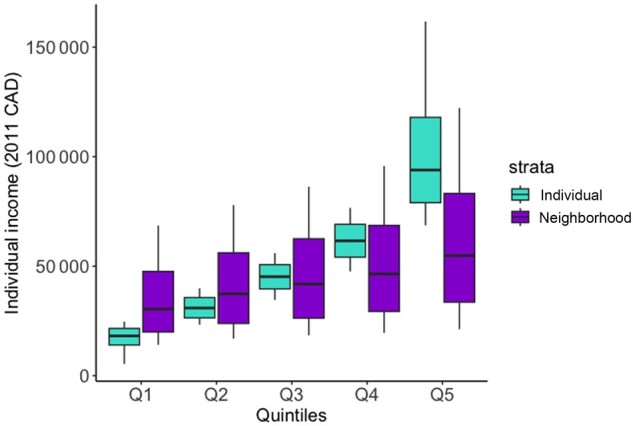
Individual income distribution by individual and neighborhood income quintiles (whiskers represent 10th and 90th percentiles as opposed to minimum and maximum values because of data confidentiality). Q = quintiles; CAD = Canadian Dollars.
Characteristics by individual and neighborhood income
A greater number of individuals with CRC were categorized in the lowest individual income quintile (Q1 = 23 145 vs Q5 = 18 715), whereas individuals were evenly spread across neighborhood income quintiles (Q1 = 20 780 vs Q5 = 20 205) (Table 3). Patients in the lowest individual income quintile were older and more likely to be female compared with those in the highest income quintile (median age = 68 years in Q1 vs 61 years in Q5; Q1 = 54% female vs Q5 = 37% female), whereas age and sex distributions were similar across neighborhood income quintiles. Patients in Q1 for both individual and neighborhood income were more likely to die during the follow-up period compared with Q5, with a greater difference by individual income (Q1 = 71% vs Q5 = 51% for individual income and Q1 = 66% vs Q5 = 57% for neighborhood income).
Table 3.
Individual characteristics by individual and neighborhood income quintiles
| Characteristics | Individual income quintiles |
Neighborhood income quintiles |
||||||||
|---|---|---|---|---|---|---|---|---|---|---|
| Q1 (lowest quintile, n = 23 145) | Q2 (n = 23 505) | Q3 (n = 19 790) | Q4 (n = 19 275) | Q5 (highest quintile, n = 18 715) | Q1 (lowest quintile, n = 20 780) | Q2 (n = 21 410) | Q3 (n = 20 735) | Q4 (n = 20 400) | Q5 (highest quintile, n = 20 205) | |
| Variable | No. (%) | No. (%) | No. (%) | No. (%) | No. (%) | No. (%) | No. (%) | No. (%) | No. (%) | No. (%) |
| Age at census, mean (SD), y | 68 (12) | 67 (12) | 64 (12) | 62 (12) | 61 (11) | 65 (12) | 65 (12) | 65 (12) | 64 (12) | 64 (12) |
| Age at census | ||||||||||
| 35-44 y | 1035 (4.7) | 1095 (4.7) | 1210 (6.1) | 1165 (6.3) | 1050 (5.6) | 1065 (5.1) | 1025 (4.8) | 1140 (5.5) | 1185 (5.8) | 1140 (5.7) |
| 45-54 y | 2220 (9.6) | 2175 (9.3) | 2800 (14.1) | 3585 (19.5) | 4465 (23.9) | 2730 (13.1) | 2865 (13.4) | 3105 (15.0) | 3245 (15.9) | 3295 (16.3) |
| 55-64 y | 4900 (21.2) | 4410 (18.8) | 4980 (25.2) | 5400 (29.4) | 6245 (33.4) | 4945 (23.8) | 5160 (24.1) | 5205 (25.1) | 5340 (26.2) | 5280 (26.1) |
| 65-74 y | 7470 (32.3) | 8840 (37.6) | 6510 (32.9) | 5100 (27.8) | 4280 (22.9) | 6630 (31.9) | 6925 (32.4) | 6355 (30.7) | 6200 (30.4) | 6085 (30.1) |
| 75-84 y | 5960 (25.7) | 5810 (24.7) | 3570 (18.0) | 2580 (14.0) | 2195 (11.7) | 4350 (20.9) | 4460 (20.8) | 4050 (19.5) | 3625 (17.8) | 3630 (18.0) |
| 85 y or older | 1560 (6.7) | 1180 (5.0) | 725 (3.7) | 550 (3.0) | 485 (2.6) | 1065 (5.1) | 975 (4.6) | 880 (4.2) | 810 (4.0) | 770 (3.8) |
| Sex | ||||||||||
| Male | 10 680 (41.2) | 13 230 (56.3) | 11 730 (59.3) | 11 040 (60.1) | 11 840 (63.3) | 11 255 (54.2) | 11 930 (55.7) | 11 740 (56.6) | 11 810 (57.9) | 11 785 (58.3) |
| Female | 12 460 (53.8) | 10 275 (43.7) | 8060 (40.7) | 7340 (39.9) | 6875 (36.7) | 9525 (45.8) | 9475 (44.3) | 9000 (43.4) | 8590 (42.1) | 8420 (41.7) |
| Province or territory at census | ||||||||||
| Newfoundland and Labrador | 545 (2.4) | 670 (2.8) | 520 (2.6) | 495 (2.7) | 445 (2.4) | 535 (2.6) | 555 (2.6) | 535 (2.6) | 575 (2.8) | 480 (2.4) |
| Prince Edward Island | 155 (0.7) | 105 (0.5) | 100 (0.5) | 125 (0.7) | 120 (0.6) | 125 (0.6) | 105 (0.5) | 125 (0.6) | 140 (0.7) | 110 (0.6) |
| Nova Scotia | 960 (4.2) | 990 (4.2) | 850 (4.3) | 745 (4.1) | 810 (4.3) | 900 (4.3) | 855 (4.0) | 880 (4.2) | 860 (4.2) | 865 (4.3) |
| New Brunswick | 655 (2.8) | 735 (3.1) | 585 (3.0) | 480 (2.6) | 525 (2.8) | 665 (3.2) | 580 (2.7) | 610 (3.0) | 570 (2.8) | 555 (2.8) |
| Quebec | 5035 (21.8) | 4810 (20.5) | 3730 (18.8) | 3320 (18.1) | 3455 (18.5) | 4525 (21.8) | 4425 (20.7) | 3995 (12.3) | 3725 (18.3) | 3675 (18.2) |
| Ontario | 8935 (38.6) | 9185 (39.1) | 7905 (39.9) | 7575 (41.2) | 7625 (40.7) | 7615 (36.7) | 8375 (39.1) | 8330 (40.2) | 8390 (41.1) | 8510 (42.1) |
| Manitoba | 970 (4.2) | 1010 (4.3) | 940 (4.7) | 845 (4.6) | 880 (4.7) | 890 (4.3) | 1045 (4.9) | 965 (4.7) | 915 (4.5) | 815 (4.0) |
| Saskatchewan | 815 (3.5) | 915 (3.9) | 735 (3.7) | 690 (3.8) | 705 (3.8) | 800 (3.8) | 810 (3.8) | 785 (3.8) | 760 (3.7) | 710 (3.5) |
| Alberta | 2080 (9.0) | 1850 (7.9) | 1630 (8.2) | 1465 (8.0) | 1535 (8.2) | 1745 (8.4) | 1760 (8.2) | 1760 (8.5) | 1655 (8.1) | 1640 (8.1) |
| British Columbia | 2910 (12.6) | 3160 (13.4) | 2730 (13.8) | 2555 (13.9) | 2540 (13.6) | 2910 (14.0) | 2830 (13.2) | 2645 (12.8) | 2740 (13.4) | 2780 (13.8) |
| Territories combined | 75 (0.3) | 80 (0.3) | 70 (0.4) | 75 (0.4) | 80 (0.4) | 70 (0.3) | 70 (0.3) | 105 (0.5) | 75 (0.4) | 65 (0.3) |
| Rural (pop < 1000) | ||||||||||
| Urban | 17 505 (75.6) | 17 560 (74.7) | 15 170 (76.7) | 14 270 (77.7) | 14 495 (77.4) | 15 935 (76.7) | 16 470 (76.9) | 15 610 (75.3) | 15 410 (75.5) | 15 580 (77.1) |
| Rural | 5640 (24.4) | 5945 (25.3) | 4620 (23.3) | 4105 (22.3) | 4220 (22.6) | 4845 (23.3) | 4940 (23.1) | 5130 (24.7) | 4995 (24.5) | 4625 (22.9) |
| Tumor location | ||||||||||
| Rectal | 7525 (32.5) | 7665 (32.6) | 6820 (34.4) | 6275 (34.1) | 6530 (34.9) | 7005 (33.7) | 7195 (33.6) | 6960 (33.6) | 6915 (33.9) | 6740 (33.4) |
| Colon | 15 615 (67.5) | 15 840 (67.4) | 12 975 (65.6) | 12 105 (65.9) | 12 180 (65.1) | 13 775 (66.3) | 14 215 (66.4) | 13 780 (66.4) | 13 485 (66.1) | 13 465 (66.7) |
| Status | ||||||||||
| Alive at end of follow-up | 6750 (29.2) | 8035 (34.2) | 8160 (41.21) | 8485 (46.2) | 9205 (59.2) | 7090 (34.1) | 8015 (37.4) | 8240 (39.7) | 8580 (42.1) | 8705 (43.1) |
| Died | 16 395 (70.8) | 15 475 (65.8) | 11 635 (58.8) | 9890 (53.8) | 9510 (50.8) | 13 690 (65.9) | 13 395 (62.6) | 12 495 (60.3) | 11 820 (57.9) | 11 500 (56.9) |
| Stage at diagnosisa | ||||||||||
| Stage 0-I | 930 (18.8) | 1285 (20.5) | 1235 (21.9) | 1190 (22.2) | 1275 (23.8) | 1030 (20.0) | 1135 (20.5) | 1185 (21.1) | 1295 (22.7) | 1270 (22.8) |
| Stage II | 1170 (23.7) | 1515 (24.2) | 1320 (23.4) | 1220 (22.8) | 1130 (21.0) | 1250 (24.2) | 1300 (23.5) | 1275 (22.7) | 1310 (23.0) | 1225 (22.0) |
| Stage III | 1210 (24.5) | 1555 (24.8) | 1505 (26.7) | 1450 (27.1) | 1460 (27.3) | 1315 (25.5) | 1450 (26.2) | 1475 (26.3) | 1495 (26.2) | 1450 (26.0) |
| Stage IV | 905 (18.4) | 1130 (18.0) | 965 (17.1) | 875 (16.3) | 920 (14.2) | 910 (17.7) | 960 (17.4) | 1000 (17.8) | 945 (16.5) | 980 (17.5) |
| Unknown | 300 (6.0) | 295 (4.7) | 220 (3.9) | 185 (3.5) | 185 (3.4) | 245 (4.8) | 245 (4.4) | 220 (3.9) | 240 (4.2) | 235 (4.2) |
| Missing | 430 (8.7) | 490 (7.8) | 405 (7.2) | 430 (8.1) | 395 (7.4) | 405 (7.9) | 445 (8.0) | 460 (8.2) | 420 (7.4) | 420 (7.6) |
Stage at diagnosis only for individuals diagnosed in 2010 or later. Q = quintile; Pop = population.
Relative and additive survival by individual and neighborhood income
Unadjusted individual income had a greater association with survival than neighborhood income when modeled separately (Q1 vs Q5 individual: HR = 1.69, RD = 50.74; neighborhood: HR = 1.20, RD = 19) (Figure 2, Table 4). After adjusting for individual covariates, the association of individual income on survival was attenuated, whereas neighborhood income remained similar (Q1 vs Q5 individual: HR = 1.36, RD = 32.23; neighborhood: HR = 1.20, RD = 19). This could indicate that confounders are not appropriately controlled for at the neighborhood level because of only controlling for individual-level covariates. To facilitate comparability between the 2 measures, unadjusted effects are reported moving forward. When both measures were included in the same model, the estimates for neighborhood income were attenuated, whereas individual income remained similar to its unadjusted estimate. This suggests that some, but not all, of the effect of neighborhood income on survival is accounted for by individual income.
Figure 2.

Five-year Kaplan–Meier survival by individual and neighborhood income quintiles.
Table 4.
Cox proportional hazards regression and Lin semiparametric hazards regression for the association between income and survival
| Model | Cox regression model |
Lin’s regression model |
||
|---|---|---|---|---|
| Unadjusted | Adjusted | Unadjusted | Adjusted | |
| HR (95% CI) | HR (95% CI) | RD (95% CI) per 1000 py | RD (95% CI) per 1000 py | |
| Individual (referent = Q5) | ||||
| Q1 | 1.69 (1.65 to 1.73) | 1.36 (1.32 to 1.39) | 50.74 (31.35 to 70.12) | 32.23 (15.49 to 48.97) |
| Q2 | 1.52 (1.48 to 1.56) | 1.23 (1.20 to 1.26) | 37.60 (19.42 to 55.77) | 19.86 (4.19 to 35.52) |
| Q3 | 1.26 (1.22 to 1.29) | 1.12 (1.09 to 1.16) | 17.99 (0.68 to 35.31) | 9.45 (-5.36 to 24.26) |
| Q4 | 1.10 (1.07 to 1.13) | 1.06 (1.03 to 1.09) | 6.86 (-9.74 to 23.46) | 4.23 (-10.15 to 18.61) |
| Neighborhood (referent = Q5) | ||||
| Q1 | 1.20 (1.17 to 1.23) | 1.20 (1.18 to 1.23) | 23.83 (4.73 to 42.94) | 19.00 (2.75 to 35.25) |
| Q2 | 1.11 (1.08 to 1.13) | 1.11 (1.08 to 1.14) | 13.69 (-4.63 to 32.00) | 9.45 (-6.15 to 25.05) |
| Q3 | 1.09 (1.06 to 1.12) | 1.09 (1.06 to 1.12) | 8.98 (-9.34 to 27.29) | 7.81 (-7.79 to 23.41) |
| Q4 | 1.04 (1.02 to 1.07) | 1.04 (1.02 to 1.07) | 3.20 (-14.33 to 20.72) | 3.60 (-11.28 to 18.48) |
| Individual and neighborhood | ||||
| Individual (referent = Q5) | ||||
| Q1 | 1.64 (1.60 to 1.69) | 1.32 (1.23 to 1.36) | 47.82 (28.43 to 67.20) | 29.50 (12.76 to 46.24) |
| Q2 | 1.49 (1.45 to 1.53) | 1.20 (1.17 to 1.24) | 35.77 (17.60 to 53.94) | 18.00 (2.34 to 33.66) |
| Q3 | 1.24 (1.21 to 1.27) | 1.11 (1.08 to 1.14) | 16.83 (-0.49 to 34.14) | 8.18 (-6.70 to 23.06) |
| Q4 | 1.09 (1.06 to 1.12) | 1.05 (1.02 to 1.08) | 6.17 (-10.36 to 22.69) | 3.47 (-10.92 to 17.86) |
| Neighborhood (referent = Q5) | ||||
| Q1 | 1.11 (1.08 to 1.14) | 1.12 (1.10 to 1.15) | 10.29 (-8.74 to 29.32) | 11.50 (-4.89 to 27.89) |
| Q2 | 1.05 (1.02 to 1.08) | 1.06 (1.03 to 1.08) | 4.38 (-13.72 to 22.48) | 4.45 (-11.21 to 20.11) |
| Q3 | 1.03 (1.00 to 1.06) | 1.05 (1.03 to 1.08) | 2.42 (-15.61 to 20.44) | 4.27 (-11.39 to 19.93) |
| Q4 | 1.00 (0.97 to 1.02) | 1.02 (1.00 to 1.05) | −0.61 (-17.85 to 16.63) | 1.53 (-13.35 to 16.41) |
| Individuala neighborhood (referent = IQ5 and NQ5) | ||||
| IQ1 and NQ1 | 1.87 (1.79 to 1.95) | 1.53 (1.47 to 1.60) | 60.48 (56.20 to 64.77) | 44.03 (34.65 to 53.40) |
| IQ2 and NQ2 | 1.62 (1.55 to 1.70) | 1.32 (1.25 to 1.38) | 42.56 (38.17 to 46.94) | 24.65 (14.75 to 34.56) |
| IQ3 and NQ3 | 1.30 (1.23 to 1.37) | 1.30 (1.23 to 1.38) | 19.71 (15.42 to 23.99) | 12.41 (2.61 to 22.21) |
| IQ4 and NQ4 | 1.12 (1.06 to 1.18) | 1.09 (1.04 to 1.15) | 7.79 (3.84 to 11.75) | 5.64 (-3.77 to 15.05) |
Adjusted models control for age, sex, tumor location, census year, province or territory at census. CI = confidence interval; HR = hazard ratio; IQ = individual quintile; NQ = neighborhood quintile; py = person years; Q = quintile; RD = risk difference.
The overall P value for the interaction between individual and neighborhood income was not statistically significant (cox P = .55); however, the individual estimates suggest some multiplicative and additive effects of individual and neighborhood income with survival. Compared with those in individual and neighborhood Q5, the most at risk for poor survival were those in the lowest individual and neighborhood income quintiles (HR for individual Q1 and neighborhood Q1 = 1.87, RD = 60.48). The presence of multiplicative and additive interaction for patients categorized with the same individual and neighborhood income quintiles suggests that these 2 indicators are measuring different concepts resulting in a joint effect on survival.
After stratifying by rural residence, individual and neighborhood income had a smaller association with survival in rural areas compared with urban areas, and additive effects for neighborhood income were not statistically significant (Supplementary Table 3, available online). Similar patterns were observed after stratifying by stage at diagnosis (Supplementary Table 4, available online).
Discussion
We found weak agreement between individual- and neighborhood-level income in Canadian CRC patients, with even weaker agreement for those residing in rural areas. Although both individual and neighborhood income were associated with survival, individual income had a stronger effect on survival, with the estimate for neighborhood income crossing the null when looking at additive effects and in rural areas. Furthermore, the presence of joint effects of individual and neighborhood income on survival suggests that these 2 measures are acting independently and jointly on outcomes.
The results from our study are in line with other studies demonstrating low agreement between individual- and neighborhood-level income measures (10-14,32). Other studies examining misclassification of the PCCF+ neighborhood income found slightly stronger agreement (10,13,14). For example, 29% and 27% perfect agreement was found by Buajitti et al. (13) and Pichora et al. (10), respectively, compared with 17% found in our study. These studies compared individual income from the Canadian Community Health Survey, which is entirely self-reported, with neighborhood income from the PCCF+, which uses a combination of self-reported and tax-reported data from the long form census (10,13). Our study used the same measures from the same populations by using the census data for both individual and neighborhood income quintiles, which could explain the difference in agreement that we observed. Moreover, our study could indicate that agreement between individual and neighborhood income is worse in the CRC population compared with the general population.
We also demonstrated lower agreement and a slightly weaker effect of individual and neighborhood income on survival in rural areas compared with nonrural areas. This is likely because of the larger geographical areas assigned to rural regions, which result in more heterogenous populations compared with smaller urban neighborhoods. This strong heterogeneity likely results in an attenuation of the effect on survival. Our study also presents relative and additive effects of individual and neighborhood income on survival, whereas other studies present only relative effects. Reporting additive effects is especially important when examining inequalities by income because they provide information about the magnitude of inequalities in a population and are more relevant to policy makers (33,34).
Presently, cancer organizations worldwide are acknowledging the pervasive inequalities in cancer outcomes by income and are calling for decreased barriers and equitable access to cancer care (35-37). However, to create successful, evidence-based interventions to reduce health inequalities by income, it is imperative to have a strong understanding of the relationship between income and cancer outcomes. Using neighborhood income as a proxy for individual income could result in an underestimation or incorrect understanding of the pathways through which income effects outcomes. This can in turn result in ineffective interventions, or even no interventions if no effect is concluded with neighborhood income alone. Interpreting neighborhood income as a measure of the individuals’ environment is also challenging. The areas used in these measures are created from administrative units, ranging from half-block radiuses in large downtown centers to hundreds of kilometers in rural areas and do not reflect human mobility and living patterns (38,39). In cases in which researchers are interested in the effect of the physical environment on cancer outcomes, more specific exposures can be used such as distance to cancer centers or greenspace exposure (40,41).
Because neighborhood income has a small effect on survival outcomes, often nearing the null, researchers should be cautious about concluding an absence of inequalities by income when individual income is not also measured. We recommend that whenever possible, individual income measures be used in cancer studies. Neighborhood income should not be used as a proxy for individual income and should instead be interpreted as an area-level measure with the caveat that it represents different sized areas depending on rural residence. A call to data custodians to make individual measures available is required, especially for widely used cancer databases such as the Surveillance, Epidemiology, and End Results and the National Cancer Database (42,43). Data confidentiality is often used as an argument for why individual measures are not provided; however, some research centers are already providing individual measures of income. For example, Statistics Canada now provides access to T1 tax files for individuals responding to the Canadian Community Health Survey (44). For researchers who do not have access to individual measures, quantitative bias analysis using validation studies in similar populations is a relatively simple method that can be used to demonstrate the changes in effect that would occur if individual income had been available (45).
There are several limitations of this study. First, income was categorized into quintiles instead of measured as a continuous variable. Modeling continuous income would avoid arbitrary cut points and increase accuracy and efficiency of the analysis. However, because most research using administrative data categorizes income as quintiles, this study demonstrates the real-world use of income. Second, individual and neighborhood income were measured on average 5 years prior to cancer diagnosis. This should have no effect on the analysis for agreement because both indicators are measured at the same time but might introduce misclassification bias for the effect of income on survival. For example, individual income might increase or decrease over those 5 years, and neighborhood income might change if participants moved to a different neighborhood. Third, we did not have a large enough sample size to detect statistically significant effects for the interaction between individual and neighborhood income; however, because specific effect sizes were statistically significant, our conclusions do not change. Finally, these results may not be generalizable outside of a Canadian setting where neighborhoods might be defined in different ways; however, the conclusion of accurately defining and interpreting income exposures remains the same.
Understanding differences between individual and neighborhood income is becoming increasingly important as we shift from understanding inequalities to implementing interventions to address inequity. This study found very poor agreement between individual and neighborhood income quintiles and much stronger associations of individual income with survival compared with neighborhood income. Cancer researchers should avoid using neighborhood income as a proxy for individual income, especially in CRC where patients might be at a higher risk of experiencing inequalities by income. In the absence of individual income measurements, researchers can use quantitative bias analysis to demonstrate the change in effect that might have occurred if individual income was available. Future work should use validation and quantitative bias analyses to demonstrate how neighborhood income can be adjusted to reflect individual income.
Supplementary Material
Contributor Information
Laura E Davis, Department of Epidemiology, Biostatistics and Occupational Health, McGill University, Montreal, Canada.
Alyson L Mahar, Faculty of Health Sciences, School of Nursing, Queens University, Kingston, Canada.
Erin C Strumpf, Department of Epidemiology, Biostatistics and Occupational Health, McGill University, Montreal, Canada; Department of Economics, McGill University, Montreal, Canada.
Funding
This study is support by grants from the Canadian Institutes of Health Research (CIHR), the Canadian Cancer Society (MEGAN-CAN), the Canadian Centre for Applied Research in Cancer Control (ARCC), and Fonds de recherche du Québec—Santé (FRQS).
Notes
Role of the funder: The funder did not play a role in the design of the study; the collection, analysis, and interpretation of the data; the writing of the manuscript; and the decision to submit the manuscript for publication.
Disclosures: The authors have no conflicts of interest.
Author contributions: Erin C. Strumpf (Conceptualization; Methodology; Supervision; Writing—review & editing), Alyson L. Mahar (Conceptualization; Methodology; Supervision; Writing—review & editing), Laura E. Davis (Conceptualization; Data curation; Formal analysis; Funding acquisition; Methodology; Visualization; Writing—original draft; Writing—review & editing).
Acknowledgements: This research was supported by funds to the Canadian Research Data Centre Network (CRDCN) from the Social Sciences and Humanities Research Council (SSHRC), the Canadian Institute for Health Research (CIHR), the Canadian Foundation for Innovation (CFI), and Statistics Canada. Although the research and analysis are based on data from Statistics Canada, the opinions expressed do not represent the views of Statistics Canada.
Data availability
The CanCHEC database is protected by Statistics Canada confidentiality policies and cannot be made publicly available. Access may be granted to those who meet prespecified criteria for confidential access available at https://www.statcan.gc.ca/en/microdata/data-centres/access.
References
- 1. Morgan E, Arnold M, Gini A, et al. Global burden of colorectal cancer in 2020 and 2040: incidence and mortality estimates from GLOBOCAN. Gut. 2023;72(2):338-44. https://gut.bmj.com/content/early/2022/09/07/gutjnl-2022-327736. Accessed November 7, 2022. [DOI] [PubMed] [Google Scholar]
- 2. Siegel RL, Miller KD, Fuchs HE, Jemal A.. Cancer statistics, 2022. CA Cancer J Clin. 2022;72(1):7-33. [DOI] [PubMed] [Google Scholar]
- 3. Manser CN, Bauerfeind P.. Impact of socioeconomic status on incidence, mortality, and survival of colorectal cancer patients: a systematic review. Gastrointest Endosc. 2014;80(1):42-60.e9. [DOI] [PubMed] [Google Scholar]
- 4. Pruitt SL, Shim MJ, Mullen PD, Vernon SW, Amick BC.. Association of area socioeconomic status and breast, cervical, and colorectal cancer screening: a systematic review. Cancer Epidemiol Biomarkers Prev. 2009;18(10):2579-2599. [DOI] [PMC free article] [PubMed] [Google Scholar]
- 5. Sinding C, Warren R, Fitzpatrick-Lewis D, Sussman J.. Research in cancer care disparities in countries with universal healthcare: mapping the field and its conceptual contours. Support Care Cancer. 2014;22(11):3101-3120. [DOI] [PubMed] [Google Scholar]
- 6. Jones JRA, Berney S, Connolly B, et al. Socioeconomic position and health outcomes following critical illness: a systematic review. Crit Care Med. 2019;47(6):e512-e521. [DOI] [PubMed] [Google Scholar]
- 7. Afshar N, English DR, Milne RL.. Factors explaining socio-economic inequalities in cancer survival: a systematic review. Cancer Control. 2021;28:1-22. [DOI] [PMC free article] [PubMed] [Google Scholar]
- 8. Mustard CA, Derksen S, Berthelot JM, Wolfson M.. Assessing ecologic proxies for household income: a comparison of household and neighborhood level income measures in the study of population health status. Health & Place. 1999;5(2):157-171. [DOI] [PubMed] [Google Scholar]
- 9. DeRouen MC, Schupp CW, Yang J, et al. Impact of individual and neighborhood factors on socioeconomic disparities in localized and advanced prostate cancer risk. Cancer Causes Control. 2018;29(10):951-966. [DOI] [PMC free article] [PubMed] [Google Scholar]
- 10. Pichora E, Polsky JY, Catley C, Perumal N, Jin J, Allin S.. Comparing individual and area-based income measures: impact on analysis of inequality in smoking, obesity, and diabetes rates in Canadians 2003–2013. Can J Public Health. 2018;109(3):410-418. [DOI] [PMC free article] [PubMed] [Google Scholar]
- 11. Shariff-Marco S, Yang J, John EM, et al. Impact of neighborhood and individual socioeconomic status on survival after breast cancer varies by race/ethnicity: the neighborhood and breast cancer study. Cancer Epidemiol Biomarkers Prev. 2014;23(5):793-811. [DOI] [PMC free article] [PubMed] [Google Scholar]
- 12. DeRouen MC, Schupp CW, Koo J, et al. Impact of individual and neighborhood factors on disparities in prostate cancer survival. Cancer Epidemiol. 2018;53:1-11. [DOI] [PMC free article] [PubMed] [Google Scholar]
- 13. Buajitti E, Chiodo S, Rosella LC.. Agreement between area- and individual-level income measures in a population-based cohort: implications for population health research. SSM Popul Health. 2020;10:100553. [DOI] [PMC free article] [PubMed] [Google Scholar]
- 14. Pampalon R, Hamel D, Gamache P.. A comparison of individual and area-based socio-economic data for monitoring social inequalities in health. Health Rep. 2009;20(4):85-94. [PubMed] [Google Scholar]
- 15. Hanley GE, Morgan S.. On the validity of area-based income measures to proxy household income. BMC Health Serv Res. 2008;8(1):79. [DOI] [PMC free article] [PubMed] [Google Scholar]
- 16. Xie S, Hubbard RA, Himes BE.. Neighborhood-level measures of socioeconomic status are more correlated with individual-level measures in urban areas compared with less urban areas. Ann Epidemiol. 2020;43:37-43.e4. [DOI] [PMC free article] [PubMed] [Google Scholar]
- 17. Narla NP, Pardo-Crespo MR, Beebe TJ, et al. Concordance between individual vs. area-level socioeconomic measures in an urban setting. J Health Care Poor Underserved. 2015;26(4):1157-1172. [DOI] [PubMed] [Google Scholar]
- 18. Pampalon R, Hamel D, Gamache P.. Health inequalities in urban and rural Canada: comparing inequalities in survival according to an individual and area-based deprivation index. Health Place. 2010;16(2):416-420. [DOI] [PubMed] [Google Scholar]
- 19. Tjepkema M, Christidis T, Bushnik T, Pinault L.. Cohort profile: the Canadian Census Health and Environment Cohorts (CanCHECs). Health Rep. 2019;30(12):18-26. [DOI] [PubMed] [Google Scholar]
- 20.Government of Canada SC. Canadian Cancer Registry (CCR). 2022. https://www23.statcan.gc.ca/imdb/p2SV.pl?Function=getSurvey&SDDS=3207. Accessed November 7, 2022.
- 21. Statistics Canada. Adjusted after-tax income of economic family. 2016. https://www23.statcan.gc.ca/imdb/p3Var.pl?Function=DEC&Id=103386. Accessed April 19, 2022.
- 22. Statistics Canada. Table 18-10-0005-01 consumer price index, annual average, not seasonally adjusted. https://www150.statcan.gc.ca/t1/tbl1/en/tv.action?pid=1810000501. Accessed June 2, 2022.
- 23. Mendelson R. Geographic Structures as Census Variables: Using Geography to Analyse Social and Economic Processes. Ottawa: Statistics Canada; 2001. https://www150.statcan.gc.ca/n1/pub/92f0138m/92f0138m2001001-eng.pdf. Accessed June 2, 2022. [Google Scholar]
- 24. Canadian Institute for Health Information. Trends in Income-Related Health Inequalities in Canada. 2015. https://secure.cihi.ca/free_products/trends_in_income_related_inequalities_in_canada_2015_en.pdf. Accessed June 2, 2022. [Google Scholar]
- 25. Wilkins R. PCCF + Version 3G Users Guide: Automated Geographic Coding Based on the Statistics Canada Postal Code Conversion Files. Cat. No. 82F0086-XDB. 2001. https://www150.statcan.gc.ca/n1/pub/92-154-g/92-154-g2017001-eng.htm. Accessed June 2, 2022.
- 26. Statistics Canada. Dissemination area: detailed definition. https://www150.statcan.gc.ca/n1/pub/92-195-x/2011001/geo/da-ad/def-eng.htm. Accessed June 2, 2022.
- 27. Canadian Institute for Health Information. Measuring health inequalities: a toolkit: area-level equity stratifiers using PCCF and PCCF+. 2018. https://www.cihi.ca/en/measuring-health-inequalities-a-toolkit. Accessed June 2, 2022.
- 28. Edge SB, Compton CC.. The American Joint Committee on Cancer: the 7th edition of the AJCC cancer staging manual and the future of TNM. Ann Surg Oncol. 2010;17(6):1471-1474. [DOI] [PubMed] [Google Scholar]
- 29. Canadian Cancer Statistics Advisory Committee. Canadian Cancer Statistics 2018. Toronto, ON: Canadian Cancer Society; 2018. https://cancer.ca/en/research/cancer-statistics/past-editions. Accessed October 2, 2018. [Google Scholar]
- 30. Cohen J. Weighted kappa: nominal scale agreement provision for scaled disagreement or partial credit. Psychol Bull. 1968;70(4):213-220. [DOI] [PubMed] [Google Scholar]
- 31. Martinussen T, Scheike TH.. Dynamic Regression Models for Survival Data. New York: Springer Science & Business Media; 2007. [Google Scholar]
- 32. Wu CC, Hsu TW, Chang CM, Yu CH, Wang YF, Lee CC.. The effect of individual and neighborhood socioeconomic status on gastric cancer survival. PLoS One. 2014;9(2):e89655. [DOI] [PMC free article] [PubMed] [Google Scholar]
- 33. King NB, Harper S, Young ME.. Use of relative and absolute effect measures in reporting health inequalities: structured review. BMJ. 2012;345:e5774. https://www.ncbi.nlm.nih.gov/pmc/articles/PMC3432634/. Accessed December 12, 2019. [DOI] [PMC free article] [PubMed] [Google Scholar]
- 34. Mahar AL, Davis LE, Kurdyak P, Hanna TP, Coburn NG, Groome PA.. Using additive and relative hazards to quantify colorectal survival inequalities for patients with a severe psychiatric illness. Ann Epidemiol. 2021. Apr 1;56:70-74. [DOI] [PubMed] [Google Scholar]
- 35. Canadian Partnership Against Cancer. Canadian Strategy for Cancer Control 2019-2029. Toronto: Canadian Partnership Against Cancer; 2018. [Google Scholar]
- 36.National Household Survey. The NHS Long Term Plan. 2019. https://www.longtermplan.nhs.uk/wp-content/uploads/2019/08/nhs-long-term-plan-version-1.2.pdf. Accessed November 4, 2022.
- 37. European Commission. Europe’s Beating Cancer Plan 2021-2030. 2021. https://health.ec.europa.eu/system/files/2022-02/eu_cancer-plan_en_0.pdf. Accessed November 4, 2022.
- 38. Lupton R. Neighborhood effects: can we measure them and does it matter? LSE STICERD Research Paper No. CASE073. 2003. https://papers.ssrn.com/abstract=1158964. Accessed October 19, 2022.
- 39. Kwan MP. The limits of the neighborhood effect: contextual uncertainties in geographic, environmental health, and social science research. Ann Am Assoc Geogr. 2018;108(6):1482-1490. [Google Scholar]
- 40. Twohig-Bennett C, Jones A.. The health benefits of the great outdoors: a systematic review and meta-analysis of greenspace exposure and health outcomes. Environ Res. 2018;166:628-637. [DOI] [PMC free article] [PubMed] [Google Scholar]
- 41. Gulwadi GB, Joseph A, Keller AB.. Exploring the impact of the physical environment on patient outcomes in ambulatory care settings. HERD. 2009;2(2):21-41. [DOI] [PubMed] [Google Scholar]
- 42. Salem ME, Puccini A, Trufan SJ, et al. Impact of sociodemographic disparities and insurance status on survival of patients with early‐onset colorectal cancer. Oncologist. 2021;26(10):e1730-e1741. [DOI] [PMC free article] [PubMed] [Google Scholar]
- 43. Dhahri A, Kaplan J, Naqvi SMH, et al. The impact of socioeconomic status on survival in stage III colon cancer patients: a retrospective cohort study using the SEER census-tract dataset. Cancer Med. 2021;10(16):5643-5652. [DOI] [PMC free article] [PubMed] [Google Scholar]
- 44.Canadian Research DataCenter. Canadian Cancer Registry Linked to Canadian Vital Statistics Death Database and DeathInformation from the T1 Personal Master File. https://crdcn.ca/data/canadian-cancer-registry-linked-to-canadian-vital-statistics-death-database-and-death-information-from-the-t1-personal-master-file/. Accessed October20, 2022. [Google Scholar]
- 45. Lash TL, Fox MP, MacLehose RF, Maldonado G, McCandless LC, Greenland S.. Good practices for quantitative bias analysis. Int J Epidemiol. 2014;43(6):1969-1985. [DOI] [PubMed] [Google Scholar]
Associated Data
This section collects any data citations, data availability statements, or supplementary materials included in this article.
Supplementary Materials
Data Availability Statement
The CanCHEC database is protected by Statistics Canada confidentiality policies and cannot be made publicly available. Access may be granted to those who meet prespecified criteria for confidential access available at https://www.statcan.gc.ca/en/microdata/data-centres/access.