A Joint Model Approach for Longitudinal Data with no Time-Zero and Time-To-Event with Competing Risks

Summary

The joint modeling of longitudinal and time-to-event data is an active area in biostatistics research. The focus of this article is on developing a modeling framework for these joint models when the longitudinal and time-to-event data do not have a meaningful time-zero. The motivating example is the study of a longitudinal assessment of station during child labor and it’s relationship to time-to-delivery. A good predictor of delivery type and timing would help obstetricians better manage the end of pregnancy and better facilitate delivery. One measure of labor progression is station, a measure of the position of the fetus’ head in relation to the pelvis of the pregnant women, may be a good marker for delivery time and type. However, women enter the hospital, where their station is closely monitored, at arbitrary points in their labor process, resulting in no clear time zero. In addition, since delivery may be of various types, the competing risks due to type need to be accounted for. We develop a joint model of longitudinal and time-to-event data for this situation. The model is formulated through shared random effects between the survival and longitudinal processes, and parameter estimation is conducted through a Bayesian approach. The model is illustrated with longitudinal data on station where the relationship between station and event-time is studied and the model is used to assess the ability of longitudinal measures of station to predict the type and timing of pregnancy. We illustrate the methodology with longitudinal data taken during labor.

1. Introduction

Understanding the relationship between longitudinal biomarkers and time-to-event has been an important area for methodological research (Rizopoulos (2012), for example). These methods have been used for both characterizing the relationship between features of the longitudinal biomarker and the event-time distribution as well as to develop dynamic predictors of clinical outcome from the repeated biomarker. This article proposes new statistical methodology for the situation where the longitudinal and survival processes have no clearly defined time zero and where there are competing risks for the time-to-event outcome. We present a shared random parameter model where the longitudinal process is linked to the event process through a series of random effects. Competing risks are incorporated by separately modeling the type and timing of the clinical event given these shared random effects.

The application of interest is on understanding the relationship between a longitudinal assessment of labor progression and the type and timing of delivery in women at the end of pregnancy. Specifically, researchers are interested in assessing the relationship between station, defined as the position of the fetuses in their mother’s pelvis, and eventual delivery type and timing. Studying this relationship would provide useful information to the obstetrician about monitoring pregnant women for station during labor. The station in labor describes the descent of the fetus into the pelvis and is often measured on a $-5$ to $+5$ scale in centimeters, where the reference point of zero refers to the point where the head crosses the midpelvis (halfway out). Since women start getting measured for station once they come to the hospital in labor, there is no clear time zero relative to their start of followup. Instead, using the point where the station value crosses zero is a natural reference point. There are different ways that a fetus can be delivered, and labor progression may influence each delivery type differently. To account for this type of competing risk, we model delivery type using a polychotomous logistic regression model and then the time-to-delivery given the delivery type. The three delivery types are spontaneous which requires no intervention, C-section, and those requiring vacuum assistance.

Figure 1 shows a series of individual profiles for women who eventually have a spontaneous delivery. The figure demonstrates that the monitoring of station begins at different points in labor. Further, the longitudinal profile appears different before and after a station value of zero.

Figure 1:

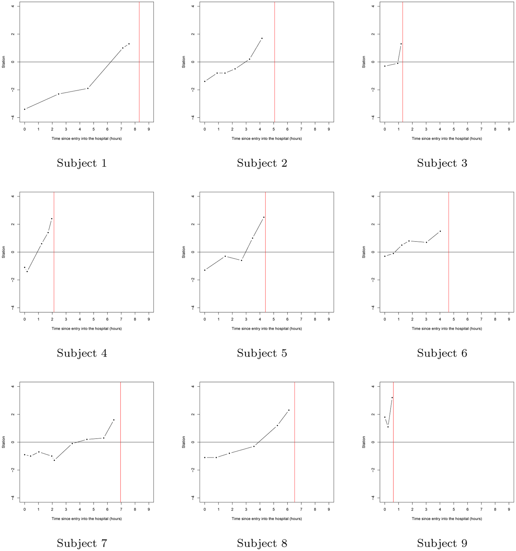
Representative station measurement trajectories resulting in a spontaneous delivery as a function of time from study entry (in hours). The red line represents the time of the spontaneous delivery.

McLain and Albert (2014) proposed a model for longitudinal data with a random change point and no-time zero that was motivated by repeat labor dilation data. The methodology was used to characterize the relationship between key demographic factors and labor progression as assessed by repeated measures of a woman’s cervical dilation. Further, this modeling strategy was used to predict future dilation measurements as well as the time to full dilation for a pregnant women based on prior dilation measurements. The current article asks a different, and perhaps the more important question of whether a repeated measure of labor progression affects the timing and type of pregnancy outcome.

In this article, we propose a joint model for longitudinal assessments of station with a random landmark and time to delivery and mode of delivery as a competing risk. We consider a shared random parameter model that links together model components for the longitudinal station process (with no time-zero) and both the time and type of delivery. Specifically, each model component includes random effects that are shared between these three components, inducing realistic dependence between these three model components. To this end, we develop an efficient Bayesian computational method for fitting this joint model via several modified collapsed Gibbs samplers (Chen et al. 2000; Liu 1994). In addition, we derive the deviance information criterion (DIC) for comparing several variations of the proposed joint models, which is a modified DIC measure when mixtures of distributions or latent variables are present.

The rest of this paper is organized as follows. In Section 2, we provide the methodological development of a flexible class of joint models for the longitudinal station measurements and the time to delivery as well as the model of delivery. This includes specifying a skewed generalized $t$-distribution for the time to delivery. In Section 3, we discuss the prediction of both the timing and type of delivery from repeated station measurements taken at various time points that can be irregularly spaced across individuals. The prior and posterior distributions, the Markov chain Monte Carlo (MCMC) sampling algorithm, and the Bayesian model comparison criteria are presented in Sections 4.1, 4.2, and 4.3, respectively. In Section 5, we apply the methodology to longitudinal labor data in order to study the association between labor dynamics and delivery time. Finally, we conclude the article with some discussion for future research in Section 6.

2. Joint Models

Suppose that $i$ denotes individual $(i=1,\dots ,I)$ and $j$ denotes time point $\left(j=1,\dots ,J_i\right)$. We assume that each measurement is taken at repeated time points, which are potentially irregularly spaced times in the delivery. Further, we assume that there are $I$ individuals in the study, each contributing $J_i$ time points, where $J_i$ denotes the number of repeated time points on the $i$th individual. Let ${\mathit{u}}_i={\left(u_{i1},\dots ,u_{i,p_1}\right)}^{\prime }$ and ${\mathit{z}}_i={\left(z_{i1},\dots ,z_{i,p_2}\right)}^{\prime }$ denote the vectors of fixed effect covariates, where ${\mathit{z}}_i$ may share common components with ${\mathit{u}}_i$. Also let $\mathit{\alpha }={\left({\alpha }_1,\dots ,{\alpha }_{p_1}\right)}^{\prime }$ and $\mathit{\gamma }={\left({\gamma }_1,\dots ,{\gamma }_{p_2}\right)}^{\prime }$ denote the corresponding regression vectors for model components of the time to delivery and the mode of delivery, respectively. In addition, $\mathit{\beta }={\left({\beta }_1,\dots ,{\beta }_{p_3}\right)}^{\prime }$ denotes the vector of regression parameters for the longitudinal measurements. Furthermore, we assume that $t_{ij}^{*}$ denotes the $j^{\text{th}}$ time for the $i^{\text{th}}$ individual after arriving at the hospital, where $t_{i1}^{*}=0$ (arriving time). Note that, since the application has three types of delivery (spontaneous, vacuum, and C-section), for ease of notation, the model is specified with three competing risks.

Let $y_{ij}$ denote the $j\text{th}$ longitudinal station measurement, $D_i$ denotes the mode of delivery such as spontaneous, vacuum, or C-section, and $S_i^{*}$ denotes the time to delivery from entry into the hospital for the $i^{\text{th}}$ individual, separatively. Note that each individual enter the hospital with different station measurement so that there is no known time zero when labor starts. Furthermore, station measurements were taken on each woman from time of entry into the hospital to a few hours before giving birth, resulting in no clear time zero for use as a reference point for valid statistical inferences and predictions. Therefore, we re-scale the $t_{ij}^{*}$ and $S_i^{*}$ such that time zero is the time when a woman’s station is zero (i.e. when a fetus is said to be engaged in the pelvis). We consider the joint models with shared random effects for the longitudinal measurements, time to delivery, and delivery type. First, we propose the following random effects regression model for the longitudinal measurements as

$$y_{ij}=\left\{\begin{array}{ll}K+{\beta }_1{t}_{ij}+{\beta }_2{t}_{ij}^2+b_{1i}{t}_{ij}+b_{2i}{t}_{ij}^2+{ϵ}_{ij}^y& \text{ if }{t}_{ij}\ge 0\\ K+{\beta }_3{t}_{ij}+b_{3i}{t}_{ij}+{ϵ}_{ij}^y& \text{ if }{t}_{ij}<0,\end{array}\right.$$ (2.1)

where $K$ is the mean station when $t_{ij}=0,t_{ij}=t_{ij}^{*}-\mu -b_{4i}$ is the re-scaled time for the $j^{\text{th}}$ station measurement on the $i^{\text{th}}$ woman with the mean time re-scaling factor $\mu$ and random effect $b_{4i}$ allowing for heterogeneity, and ${ϵ}_{ij}^y$ are random variables for the error distributions. A station value of zero, the point at which the head of the fetus crosses the mid-pelvis, is a natural reference choice; thus, $K=0$. Furthermore, $b_{1i},b_{2i}$, and $b_{3i}$ are individual-level random effects, characterizing heterogeneity in the station process across women. Let ${\mathit{ϵ}}_i^y={\left({ϵ}_i^y,\dots ,{ϵ}_{i,J_i}^y\right)}^{\prime }$ and ${\mathit{b}}_i={\left(b_{1i},b_{2i},b_{3i},b_{4i}\right)}^{\prime }$. In (2.1), we assume that (i) ${\mathit{ϵ}}_i^y$ and ${\mathit{b}}_i$ are independent; (ii) ${ϵ}_{ij}^y$ follows a normal distribution with mean 0 and variance ${\sigma }_y^2$; and (iii) the shared random effect ${\mathit{b}}_i$ follows a multivariate normal distribution mean $0$ and $4\times 4$ unstructured variance-covariance matrix $\Omega$ for $i=1,\dots ,I$ and $j=1,\dots ,J_i$. Furthermore, we assume quadratic trend after station zero and a linear form before and set $K=0$. Let $\mathit{y}={\left(y_{11},\dots ,y_{I,J_I}\right)}^{\prime },{\mathit{t}}^{*}={\left(t_{11}^{*},\dots ,t_{I,J_I}^{*}\right)}^{\prime },\mathit{ }\mathit{t}={\left(t_{11},\dots ,t_{I,J_I}\right)}^{\prime }$, and $\mathit{b}={\left({\mathit{b}}_1,\dots ,{\mathit{b}}_I\right)}^{\prime }$. Also let $D_{obs}^y=\left(\mathit{y},{\mathit{t}}^{*}\right)$ denote the observed data. Given $\mathit{b}$ and $D_{obs}^y$, the likelihood function of $\left(\mu ,\mathit{\beta },{\sigma }_y^2\right)$ for longitudinal station measurements is given by

$$L_y\left(\mu ,\mathit{\beta },{\sigma }_y^2\mid \mathit{b},D_{obs}^y\right)=\prod _{i=1}\prod _{j=1}N\left(y_{ij}\mid {\mu }_{y_{ij}},{\sigma }_y^2\right),$$ (2.2)

where ${\mu }_{y_{ij}}={\beta }_1{t}_{ij}+{\beta }_2{t}_{ij}^2+b_{1i}{t}_{ij}+b_{2i}{t}_{ij}^2$ for $t_{ij}\ge 0$ and ${\mu }_{y_{ij}}={\beta }_3{t}_{ij}+b_{3i}{t}_{ij}$ for $t_{ij}<0$. Note that $N(\cdot \mid a,b)$ denotes a normal distribution with mean $a$ and variance $b$.

For time to delivery, we propose the following flexible regression model as

$$S_i={\mathit{u}}_i^{\prime }\mathit{\alpha }+b_{1i}{\theta }_1+b_{2i}{\theta }_2+b_{3i}{\theta }_3+D_{i1}{\theta }_4+D_{i2}{\theta }_5+{ϵ}_i^S,$$ (2.3)

where $S_i=S_i^{*}-\mu -b_{4i}$ is the re-scaled time to delivery for the $i^{th}$ woman, $\mathit{\theta }=\left({\theta }_1,\dots ,{\theta }_5\right)$ are shared parameters accounting for correlation between ${\mathit{y}}_i,S_i$, and $D_i={\left(D_{i1},D_{i2}\right)}^{\prime }$ which is dichotomized. We assume that ${ϵ}_i^S$ and ${\mathit{b}}_i$ are independent, and ${ϵ}_i^S$ are random variables for the flexible error distributions that will allow for long-tailed and skewed distributions. In this paper, we propose to use long-tailed and skewed distributions to accomplish this goal. We model

$${ϵ}_i^S=\delta \left({\xi }_i-E\left({\xi }_i\right)\right)+{\eta }_i,$$ (2.4)

where the first and second terms in (2.4) characterize skewness and long tails, respectively. Similar to Kim et al. (2008), we assume that (i) ${\xi }_i$ and ${\eta }_i$ are independent; (ii) ${\xi }_i~G_{\xi }$ are each independent, where $G_{\xi }$ is the cumulative density function (cdf) of a skewed distribution defined on $R^{+}=(0,\infty )$; and (iii) ${\eta }_i$ follows a symmetric distribution. Also in (2.4), $\delta$ is a skewness parameter, where $\delta =0$ reflects a symmetric distribution. Following Chen et al. (1999) and Kim et al. (2008), we assume that $G_{\xi }$ has a known cdfs in order to ensure model identifiability. In this paper, we first specify several different distributions for $G_{\xi }$, and use the DIC (Spiegelhalter et al. (2002)) to determine which $G_{\xi }$ fits the data best. We consider the following distributions for $G_{\xi }:$ (a) $G_{\xi }$ is degenerated at 0, denoted by ${\Delta }_{\left\{0\right\}}$, yielding a symmetric distribution; (b) $G_{\xi }$ is a standard exponential distribution $\left(ℰ\right)$ with probability density function (pdf) $f_{ℰ}\left({\xi }_i\right)=\text{exp} \left(-{\xi }_i\right)$ if ${\xi }_i>0$ and 0 otherwise; and (c) $G_{\xi }$ is a half normal $\left(\mathscr{H}𝒩\right)$ with pdf $f_{\mathscr{H}𝒩}\left({\xi }_i\right)=\frac{2}{\sqrt{2\pi }}\text{exp} \left(-{\xi }_i^2/2\right)$ if ${\xi }_i>0$ and 0 otherwise. Thus given $G_{\xi }$, the model (2.4) yields a skewed distribution. Furthermore, we propose a skewed generalized $t$ model for $S_i$, which is motivated by Kim et al. (2008) for a binary response data in a generalized linear model. Let $f_{gt,{\nu }_1,{\nu }_2}\left({\eta }_i\right)$ denote the pdf of a generalized $t$-distribution (Abranowitz and Stegun (1972)) that is given by

$$f_{gt,{\nu }_1,{\nu }_2}\left({\eta }_i\right)=\frac{1}{\sqrt{\pi {\nu }_2}}\frac{\Gamma \left(\frac{{\nu }_1+1}{2}\right)}{\Gamma \left(\frac{{\nu }_1}{2}\right)}\times {\left(1+\frac{{\eta }_i^2}{{\nu }_2}\right)}^{-\frac{{\nu }_1+1}{2}},$$ (2.5)

where ${\nu }_1$ is a shape (or degrees of freedom) and ${\nu }_2$ is a scale parameter. Let ${\eta }_i~f_{gt,{\nu }_1,{\nu }_2}$, then $E\left({\eta }_i\right)=0$ for ${\nu }_1>1$ and $\text{Var} \left({\eta }_i\right)={\nu }_2/\left({\nu }_1-2\right)$ for ${\nu }_1>2$. To ensure identifiability, we assume ${\nu }_2$ to be 1 (Kim et al. 2008). We note that based on (2.5), ${ϵ}_i^S$ in (2.4) leads to a skewed generalized $t$-distribution for $S_i$. The models defined in (2.3), (2.4), and (2.5) are general and flexible, which includes the normal and skewed $t$ models as special cases. Figure 2 illustrates the skewed generalized $t$-distribution for positive, negative, and no skewness.

Figure 2:

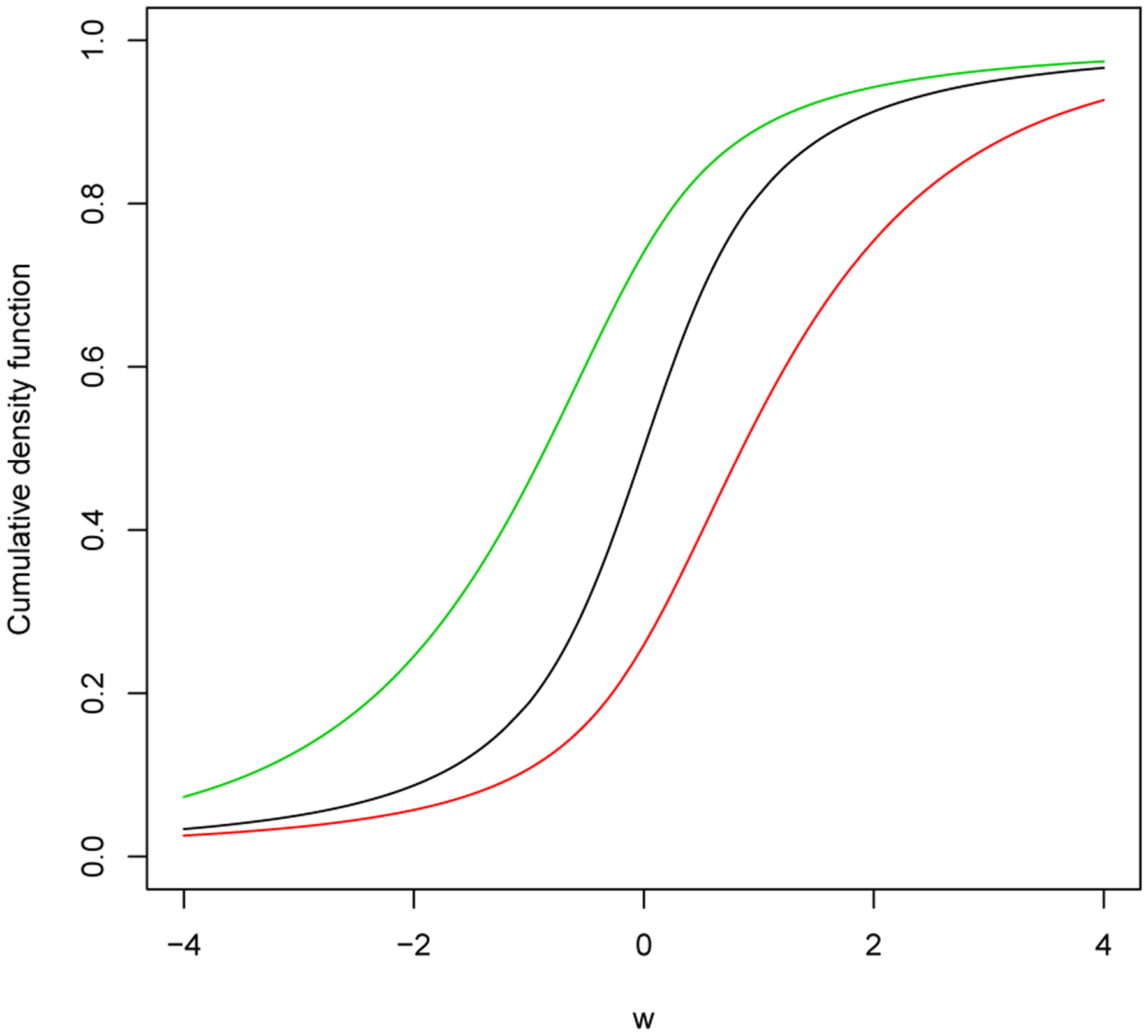
CDF plots of the skewed generalized $t$-distribution. Black line: symmetric, Red line: positive skewed, and Green line: negative skewed.

Let $\mathit{S}={\left(S_1,\dots ,S_I\right)}^{\prime },{\mathit{S}}^{*}={\left(S_1^{*},\dots ,S_I^{*}\right)}^{\prime },U={\left({\mathit{u}}_1^{\prime },\dots ,{\mathit{u}}_I^{\prime }\right)}^{\prime },{\mathit{D}}_1={\left(D_{11},\dots ,D_{I1}\right)}^{\prime }$, and ${\mathit{D}}_2={\left(D_{12},\dots ,D_{I2}\right)}^{\prime }$. Also let $D_{obs}^D=\left({\mathit{S}}^{*},U,{\mathit{D}}_1,{\mathit{D}}_2\right)$ denote the observed data. Given $\mathit{b}$ and $D_{obs}^S$, the likelihood function of $\left(\mu ,\mathit{\alpha },\mathit{\theta },\delta ,{\nu }_1,{\sigma }_S^2\right)$ for time to delivery is given by

$$L_S\left(\mu ,\mathit{\alpha },\mathit{\theta },\delta ,{\nu }_1,{\sigma }_S^2\mid \mathit{b},D_{obs}^S\right)=\prod _{i=1}\int f_{gt,{\nu }_1,{\nu }_2=1}\left(S_i\mid {\mu }_{S_i},{\sigma }_S^2\right)d{G}_{\xi }\left({\xi }_i\right),$$ (2.6)

where ${\mu }_{S_i}={\mathit{u}}_i^{\prime }\mathit{\alpha }+b_{1i}{\theta }_1+b_{2i}{\theta }_2+b_{3i}{\theta }_3+D_{i1}{\theta }_4+D_{i2}{\theta }_5+\delta \left({\xi }_i-E\left({\xi }_i\right)\right)$. Note that $f_{gt,{\nu }_1,{\nu }_2=1}(\cdot \mid a,b)$ denotes a pdf of generalized $t$-distribution with mean $a$, variance $b,{\nu }_1$ and ${\nu }_2=1$.

For the mode of delivery, we assume the multinomial logistic regression model as

$$P\left(D_i=l\mid \mathit{z},\mathit{b}\right)=\frac{\text{exp} \left({\mathit{z}}_i^{\prime }{\gamma }_l+b_{1i}{\varphi }_{l1}+b_{2i}{\varphi }_{l2}+b_{3i}{\varphi }_{l3}\right)}{1+\sum _{m=1}^{L-1}\text{exp} \left({\mathit{z}}_i^{\prime }{\mathit{\gamma }}_m+b_{1i}{\varphi }_{m1}+b_{2i}{\varphi }_{m2}+b_{3i}{\varphi }_{m3}\right)},$$ (2.7)

where ${\mathit{\varphi }}_l={\left({\varphi }_{l1},{\varphi }_{l2},{\varphi }_{l3}\right)}^{\prime }$ are shared parameters accounting for correlation between ${\mathit{y}}_i,S_i$, and $D_i,l=1,\dots ,L-1$. Note that ${\mathit{\varphi }}_L=0$. Let $\mathit{D}={\left(D_1,\dots ,D_I\right)}^{\prime },\mathit{Z}={\left({\mathit{z}}_1^{\prime },\dots ,{\mathit{z}}_I^{\prime }\right)}^{\prime }$, $\gamma ={\left({\gamma }_1^{\prime },\dots ,{\gamma }_{L-1}^{\prime }\right)}^{\prime }$, and $\mathit{\varphi }={\left({\varphi }_1^{\prime },\dots ,{\mathit{\varphi }}_{L-1}^{\prime }\right)}^{\prime }$. Also let $D_{obs}^D=(\mathit{D},Z)$ denote observed data. Given $\mathit{b}$ and $D_{obs}^D$, the likelihood function of $(\mathit{\gamma },\mathit{\varphi })$ for time to delivery is given by

$$L_D\left(\mathit{\gamma },\mathit{\varphi }\mid \mathit{b},D_{obs}^D\right)=\prod _{i=1}\prod _{l=L}P{\left(D_i=l\mid \mathit{z},\mathit{b}\right)}^{1\left(D_i=l\right)},$$ (2.8)

where $P\left(D_i=l\mid \mathit{z},\mathit{b}\right)$ is given in (2.7) and $1\left(a\right)$ is an indicator function, which is defined as $1\left(a\right)=1$ of $a$ is true and 0 otherwise.

The observed joint likelihood function of $\left(\mu ,\mathit{\beta },{\sigma }_y^2,\mathit{\alpha },\mathit{\theta },\delta ,{\nu }_1,{\sigma }_S^2,\mathit{\gamma },\mathit{\varphi }\right)$ is

$$\begin{gathered} L\left(\mu ,\mathit{\beta },{\sigma }_y^2,\mathit{\alpha },\mathit{\theta },\delta ,{\nu }_1,{\sigma }_S^2,\mathit{\gamma },\mathit{\varphi },\Omega \mid D_{obs}^y,D_{obs}^S,D_{obs}^D\right) \\ =\int L_y\left(\mu ,\mathit{\beta },{\sigma }_y^2\mid \mathit{b},D_{obs}^y\right)\times L_S\left(\mu ,\mathit{\alpha },\mathit{\theta },\delta ,{\nu }_1,{\sigma }_S^2\mid \mathit{b},D_{obs}^S\right)\times L_D\left(\mathit{\gamma },\mathit{\varphi }\mid \mathit{b},D_{obs}^D\right) \\ \times \prod _{i=1}N\left({\mathit{b}}_i\mid 0,\Omega \right)d\mathit{b}, \end{gathered}$$ (2.9)

where $L_y\left(\mu ,\mathit{\beta },{\sigma }_y^2\mid \mathit{b},D_{obs}^y\right),L_S\left(\mu ,\mathit{\alpha },\mathit{\theta },\delta ,{\nu }_1,{\sigma }_S^2\mid \mathit{b},D_{obs}^S\right)$, and $L_D\left(\mathit{\gamma },\mathit{\varphi }\mid \mathit{b},D_{obs}^D\right)$ are given in (2.2), (2.6), and (2.8), respectively. Since it is not easy to work directly with the observed joint likelihood function of $\left(\mu ,\mathit{\beta },{\sigma }_y^2,\mathit{\alpha },\mathit{\theta },\delta ,{\nu }_1,{\sigma }_S^2,\mathit{\gamma },\mathit{\varphi }\right)$ in (2.9), we develop an efficient MCMC algorithm using the fact that the generalized $t$-distribution can be represented as a gamma mixture of normal distributions for ${ϵ}_i^S$ as described in Section 4.2.

3. Predicting the time to delivery and delivery type

The joint model in (2.1), (2.3), and (2.7) relates the longitudinal station patterns to the probability of a delivery type and time to delivery through an individual’s predicted station measurement, and can be used to develop a predictor of the timing and delivery type using individualized longitudinal assessments of station. To predict the time to delivery and mode of delivery at birth using the longitudinal station measurements, we let ${\mathit{y}}^p=\left(y_{t_1},\dots ,y_{t_M}\right)$ denote the longitudinal station measurement taken at time points $t_1,\dots ,t_M$, where $M$ is the number of repeated measurements in the predictor. Furthermore, let $S^p$ and $D^p$ denote the time to delivery and mode of delivery we wish to predict. Also let $\Theta =\left(\mu ,\mathit{\beta },{\sigma }_y^2,\mathit{\alpha },\mathit{\theta },\delta ,{\nu }_1,{\sigma }_S^2,\mathit{\gamma },\mathit{\varphi }\right)$. Then the posterior predictive probability for $D^p$ and posterior predictive distribution for $S^p$ based on longitudinal measurements ${\mathit{y}}^p$ can be given by

$$\begin{gathered} P\left(D^p=l\mid {\mathit{y}}^p\right)=\int P\left(D^p=l\mid \mathit{z},{\mathit{b}}^p\right)\pi \left(\Theta ,{\mathit{b}}^p\mid {\mathit{y}}^p\right)d{\mathit{b}}^{p}d\Theta , \\ \pi \left(S^p\mid {\mathit{y}}^p\right)=\int f_{gt,{\nu }_1,{\nu }_2=1}\left(S^p\mid {\mu }_{S^p},{\sigma }_S^2\right)\pi \left(\Theta ,{\mathit{b}}^p\mid {\mathit{y}}^p\right)d{\mathit{b}}^{p}d\Theta , \end{gathered}$$ (3.1)

where ${\mu }_{S^p}={\mathit{u}}^{\prime }\mathit{\alpha }+b_1^p{\theta }_1+b_2^p{\theta }_2+b_3^p{\theta }_3+D_1^p{\theta }_4+D_2^p{\theta }_5+\delta (\xi -E(\xi \left)\right),{\mathit{b}}^p$ is a multivariate random effects $\left({\mathit{b}}^p~N(0,\Omega )\right)$ and $\pi \left(\Theta ,{\mathit{b}}^p\mid {\mathit{y}}^p\right)$ is the posterior distribution for $\Theta$ and ${\mathit{b}}^p$ based on ${\mathit{y}}^p$. To obtain the posterior predictive probability for $D^p$ and posterior predictive distribution for $S^p$ in (3.1), we sample ${\mathit{b}}^p$ from joint posterior distribution based on test set data (with parameter estimates using training dataset). Specifically, to evaluate the prediction accuracy, we divide the data into a training and test set data. Note that mode of delivery is treated as a competing risk for predicting $S^p$.

4. Posterior inference

4.1. Prior and posterior distributions

We assume that $\mu ,\mathit{\beta },{\sigma }_y^2,\mathit{\alpha },\mathit{\theta },\delta ,{\nu }_1,{\sigma }_S^2,\mathit{\gamma },\mathit{\varphi }$, and $\Omega$ are independent a priori. The priors that we assume have as weak information as possible so that the data can dominate the posterior computation. Specifically, we assume that, $\mu ~N\left(0,{\sigma }_{\mu }^2\right),\mathit{\alpha }~N_{p_1}\left(0,{\sigma }_{\alpha }^{2}I\right) \gamma ~N_{p_2}\left(0,{\sigma }_{\gamma }^{2}I\right),\mathit{\beta }~N_{p_3}\left(0,{\sigma }_{\beta }^{2}I\right),\mathit{\theta }~N_5\left(0,{\sigma }_{\theta }^{2}I\right),\mathit{\varphi }~N_3\left(0,{\sigma }_{\varphi }^{2}I\right),\delta ~N\left(0,{\sigma }_{\delta }^2\right),{\nu }_1~\text{Gamma} \left(a_1,b_1\right),{\sigma }_y^2~\text{IG} \left(a_2,b_2\right),{\sigma }_S^2~\text{IG} \left(a_3,b_3\right)$, and ${\Omega }^{-1}~\mathit{\text{Wishart}} \left(d_0,d_0{V}_0\right)$, where ${\sigma }_{\mu }^2$, ${\sigma }_{\alpha }^2,{\sigma }_{\gamma }^2,{\sigma }_{\beta }^2,{\sigma }_{\theta }^2,{\sigma }_{\varphi }^2,{\sigma }_{\delta }^2,a_1,b_1,a_2,b_2,a_3,b_3,d_0$, and $V_0$, are the prespecified hyperparameters. Note that Gamma $(a,b)$ is a Gamma distribution with mean $a/b,\text{IG} (a,b)$ is an Inverse-gamma distribution with mean $b/(a-1)$, and $\mathit{\text{Wishart}} (d,V)$ denotes a Wishart prior distribution with $d$ degrees of freedom and mean $dV$. The hyperparameters of the prior were specified as ${\sigma }_{\mu }^2=100,{\sigma }_{\alpha }^2=100,{\sigma }_{\gamma }^2=100,{\sigma }_{\beta }^2=100,{\sigma }_{\theta }^2=100,{\sigma }_{\varphi }^2=100,{\sigma }_{\delta }^2=100,a_1=1,b_1=0.1,a_2=2,b_2=1,a_3=2,b_3=1,d_0=4.1$, and $V_0=0.1I$ in the analysis. These choices of hyperparameters lead to noninformative priors. Let $D_{obs}=\left(D_{obs}^y,D_{obs}^S,D_{obs}^D\right)$. Based on the prior distributions specified above, the joint posterior distribution of $\mu ,\mathit{\beta },{\sigma }_y^2,\mathit{\alpha },\mathit{\theta },\delta ,{\nu }_1,{\sigma }_S^2,\mathit{\gamma },\mathit{\varphi }$, and $\Omega$ is thus given by

$$\begin{gathered} \pi \left(\mu ,\mathit{\beta },{\sigma }_y^2,\mathit{\alpha },\mathit{\theta },\delta ,{\nu }_1,{\sigma }_S^2,\mathit{\gamma },\mathit{\varphi },\Omega \mid D_{obs}\right) \\ =L\left(\mu ,\mathit{\beta },{\sigma }_y^2,\mathit{\alpha },\mathit{\theta },\delta ,{\nu }_1,{\sigma }_S^2,\mathit{\gamma },\mathit{\varphi },\Omega \mid D_{obs}\right) \\ \times \pi \left(\mu \right)\pi \left(\mathit{\beta }\right)\pi \left({\sigma }_y^2\right)\pi \left(\mathit{\alpha }\right)\pi \left(\mathit{\theta }\right)\pi \left(\delta \right)\pi \left({\nu }_1\right)\pi \left({\sigma }_S^2\right)\pi \left(\mathit{\gamma }\right)\pi \left(\mathit{\varphi }\right)\pi \left(\Omega \right), \end{gathered}$$ (4.1)

where $L\left(\mu ,\mathit{\beta },{\sigma }_y^2,\mathit{\alpha },\mathit{\theta },\delta ,{\nu }_1,{\sigma }_S^2,\mathit{\gamma },\mathit{\varphi },\Omega \mid D_{obs}\right)$ is defined in (2.9). We can generate a sample from this joint posterior distribution using Gibbs sampler and make appropriate inference of the various model parameters. A description of the MCMC algorithm is given in Section 4.2.

4.2. Computational Developments

The analytical evaluation of the posterior distribution of $\Theta =\left(\mu ,\mathit{\beta },{\sigma }_y^2,\mathit{\alpha },\mathit{\theta },\delta ,{\nu }_1,{\sigma }_S^2,\mathit{\gamma },\mathit{\varphi }\right.,\Omega )$ given in (4.1) is not available. However, we can develop an efficient MCMC sampling algorithm to sample from (4.1). For ease of presentation, we consider the standard exponential distribution $\left(ℰ\right)$ for $G_{\xi }$ only as the MCMC sampling algorithms for other choices of $G_{\xi }$ are similar. Since it is difficult to work directly with the observed joint likelihood function of $\Theta$ in (2.9), we use the complete data joint likelihood function of $\Theta$ using the fact that the generalized $t$-distribution can be represented as a gamma mixture of normal distributions for ${ϵ}_i^S:{\eta }_i\mid {\lambda }_i~N\left(\mathrm{0,1}/{\lambda }_i\right)$ and ${\lambda }_i~\text{Gamma} \left({\nu }_1/\mathrm{2,1}/2\right)$, where ${\lambda }_i$ is a mixing variable. Let $\mathit{\xi }={\left({\xi }_1,\dots ,{\xi }_I\right)}^{\prime }$ and $\mathit{\lambda }={\left({\lambda }_1,\dots ,{\lambda }_I\right)}^{\prime }$. Also let $D_c=\left(\mathit{t},\mathit{S},\mathit{b},\mathit{\xi },\mathit{\lambda },D_{obs}\right)$ denote complete data set. The joint posterior distribution of $\Theta$ based on the complete data joint likelihood function can be written as

$$\begin{gathered} \pi \left(\Theta \mid D_c\right) \\ \propto \prod _{i=1}\prod _{j=1}{\left({\sigma }_y^2\right)}^{-\frac{1}{2}}\text{exp} \left(-\frac{1}{2{\sigma }_y^2}{\left(y_{ij}-{\mu }_{y_{ij}}\right)}^2\right) \\ \times \prod _{i=1}{\left(\frac{{\sigma }_S^2}{{\lambda }_i}\right)}^{-\frac{{\nu }_1}{2}}\text{exp} \left(-\frac{{\lambda }_i}{2{\sigma }_S^2}{\left(S_i-{\mu }_{S_i}\right)}^2\right)\times \text{exp} \left(-{\xi }_i\right)\times \frac{2^{-\frac{{\nu }_1}{2}}}{\Gamma \left(\frac{{\nu }_1}{2}\right)}{\lambda }_i^{\frac{{\nu }_1}{2}-1}\text{exp} \left(-\frac{1}{2}{\lambda }_i\right) \\ \times \prod _{i=1}\frac{\text{exp} \left(\sum _{l=1}^{L-1}1\left(D_i=l\right)\left({\mathit{z}}_i^{\prime }{\gamma }_l+b_{1i}{\varphi }_{l1}+b_{2i}{\varphi }_{l2}+b_{3i}{\varphi }_{l3}\right)\right)}{1+\sum _{m=1}^{L-1}\text{exp} \left({\mathit{z}}_i^{\prime }{\mathit{\gamma }}_m+b_{1i}{\varphi }_{m1}+b_{2i}{\varphi }_{m2}+b_{3i}{\varphi }_{m3}\right)} \\ \times \prod _{i=1}|\Omega {|}^{-\frac{1}{2}}\text{exp} \left(-\frac{1}{2}{\mathit{b}}_i^{\prime }{\Omega }^{-1/2}{\mathit{b}}_i\right) \\ \times \pi \left(\Theta \right), \end{gathered}$$ (4.2)

where ${\mu }_{y_{ij}},{\mu }_{S_i}$, and $\pi \left(\Theta \right)$ are given in (2.2), (2.6), and (4.1), respectively. From (4.2), the algorithm requires sampling the following parameters in turn from their respective full conditional distributions: (I) $\left[{\xi }_i\mid \mu ,\mathit{\beta },{\sigma }_y^2,\mathit{\alpha },\mathit{\theta },\delta ,{\nu }_1,{\sigma }_S^2,\mathit{\gamma },\mathit{\varphi },\mathit{t},\mathit{S},\mathit{b},\mathit{\lambda },\Omega ,D_{obs}\right]$; $\left[\Omega \mid \mu ,\mathit{\beta },{\sigma }_y^2,\mathit{\alpha },\mathit{\theta },\delta ,{\nu }_1,{\sigma }_S^2,\mathit{\gamma },\mathit{\varphi },\mathit{t},\mathit{S},\mathit{b},\mathit{\xi },\mathit{\lambda },D_{obs}\right];$ (III) $\left[\mathit{\gamma },\mathit{\varphi }\mid \mu ,\mathit{\beta },{\sigma }_y^2,\mathit{\alpha },\mathit{\theta },\delta ,{\nu }_1,{\sigma }_S^2,\mathit{t},\mathit{S},\mathit{b}\right.,\left.\mathit{\xi },\mathit{\lambda },\Omega ,D_{obs}\right];$ and (IV) $\left[\mu ,\mathit{\beta },{\sigma }_y^2,\mathit{\alpha },\mathit{\theta },\delta ,{\nu }_1,{\sigma }_S^2,\mathit{b},\mathit{\lambda }\mid \mathit{\gamma },\mathit{\varphi },\mathit{t},\mathit{S},\mathit{\xi },\Omega ,D_{obs}\right]$. Let ${\mathit{x}}_i=\left({\mathit{u}}_i^{\prime },b_{1i}\right.,{\left.b_{2i},b_{3i},D_{i1},D_{i2}\right)}^{\prime },X={\left({\mathit{x}}_1^{\prime },\dots ,{\mathit{x}}_I^{\prime }\right)}^{\prime },{\mathit{w}}_i={\left({\mathit{z}}_i^{\prime },b_{1i},b_{2i},b_{3i}\right)}^{\prime },W={\left({\mathit{w}}_1,\dots ,{\mathit{w}}_I\right)}^{\prime },\mathit{\psi }={\left({\mathit{\alpha }}^{\prime },{\mathit{\theta }}^{\prime }\right)}^{\prime },{\mathit{\phi }}_l={\left({\gamma }_l^{\prime },{\mathit{\varphi }}_l^{\prime }\right)}^{\prime }$, and $\mathit{\phi }={\left({\mathit{\phi }}_1,\dots ,{\mathit{\phi }}_{L-1}\right)}^{\prime }$. For (I), observed that

$${\xi }_i\mid \mu ,\mathit{\beta },{\sigma }_y^2,\mathit{\alpha },\mathit{\theta },\delta ,{\nu }_1,{\sigma }_S^2,\mathit{\gamma },\mathit{\varphi },\mathit{t},\mathit{S},\mathit{b},\mathit{\lambda },\Omega ,D_{obs}~N\left(A_{{\xi }_i}^{-1}{B}_{{\xi }_i},A_{{\xi }_i}^{-1}\right)1\left({\xi }_i>0\right),$$ (4.3)

where $B_{{\xi }_i}={\lambda }_i\left(S_i-{\mathit{x}}_i^{\prime }\mathit{\psi }+\delta E\left({\xi }_i\right)\right)\delta /{\sigma }_S^2-1$ and $A_{{\xi }_i}={\lambda }_i{\delta }^2/{\sigma }_S^2$ for $i=1,\dots ,I$. For (II), we observe that

$$\begin{gathered} {\Omega }^{-1}\mid \mu ,\mathit{\beta },{\sigma }_y^2,\mathit{\alpha },\mathit{\theta },\delta ,{\nu }_1,{\sigma }_S^2,\mathit{\gamma },\mathit{\varphi },\mathit{t},\mathit{S},\mathit{b},\mathit{\xi },\mathit{\lambda },D_{obs} \\ ~{\text{ Wishart }}_4\left(d_0+I,{\left(d_0{V}_0^{-1}+\sum _i{\mathit{b}}_i{\mathit{b}}_i^{\prime }\right)}^{-1}\right). \end{gathered}$$ (4.4)

For (III), the conditional posterior densities for $\mathit{\phi }$ do not have closed form. Therefore, we use the Metropolis-Hastings algorithm (Hastings (1970)) to sample $\mathit{\phi }$ from their conditional posterior distributions. For (IV), we apply the collapsed Gibbs technique of Liu (1994) via the following identity:

$$\begin{gathered} \left[\mu ,\mathit{\beta },{\sigma }_y^2,\mathit{\alpha },\mathit{\theta },\delta ,{\nu }_1,{\sigma }_S^2,\mathit{b},\mathit{\lambda }\mid \mathit{\gamma },\mathit{\varphi },\mathit{t},\mathit{S},\mathit{\xi },\Omega ,D_{obs}\right] \\ =\left[{\sigma }_y^2,\mathit{\lambda }\mid \mu ,\mathit{\beta },\mathit{\alpha },\mathit{\theta },\delta ,{\nu }_1,{\sigma }_S^2,\mathit{\gamma },\mathit{\varphi },\mathit{t},\mathit{S},\mathit{b},\mathit{\xi },\Omega ,D_{obs}\right] \\ \times \left[\mu ,\mathit{\beta },\mathit{\alpha },\mathit{\theta },\delta ,{\nu }_1,{\sigma }_S^2,\mathit{b}\mid \mathit{\gamma },\mathit{\varphi },\mathit{t},\mathit{S},\mathit{\xi },\Omega ,D_{obs}\right]. \end{gathered}$$

That is, we sample $\mu ,\mathit{\beta },\mathit{\alpha },\mathit{\theta },\delta ,{\nu }_1,{\sigma }_S^2$, and $\mathit{b}$ after collapsing out ${\sigma }_y^2$ and $\mathit{\lambda }$. Observe that

$$\begin{gathered} {\sigma }_y^2\mid \mu ,\mathit{\beta },\mathit{\alpha },\mathit{\theta },\delta ,{\nu }_1,{\sigma }_S^2,\mathit{\gamma },\mathit{\varphi },\mathit{t},\mathit{S},\mathit{b},\mathit{\xi },\mathit{\lambda },\Omega ,D_{obs} \\ ~\text{IG}\left(a_2+\frac{1}{2}\sum _i{J}_i,b_2+\frac{1}{2}\sum _i\sum _j{\left(y_{ij}-{\mu }_{y_{ij}}\right)}^2\right), \end{gathered}$$ (4.5)

where ${\mu }_{y_{ij}}$ is given in (2.2). We also observe that

$$\begin{gathered} {\lambda }_i\mid \mu ,\mathit{\beta },{\sigma }_y^2,\mathit{\alpha },\mathit{\theta },\delta ,{\nu }_1,{\sigma }_S^2,\mathit{\gamma },\mathit{\varphi },\mathit{t},\mathit{S},\mathit{b},\mathit{\xi },\Omega ,D_{obs} \\ ~\text{Gamma} \left(\frac{1}{2}\left({\nu }_1+1\right),\frac{1}{2}\left(1+\frac{{\left(S_i-{\mu }_{S_i}\right)}^2}{{\sigma }_S^2}\right)\right), \end{gathered}$$ (4.6)

where $S_i$ and ${\mu }_{S_i}$ are given in (2.3). The conditional posterior densities for $\mu ,\mathit{\beta },\mathit{\psi },\delta ,{\nu }_1,{\sigma }_S^2$, and $\mathit{b}$ do not have closed form. Therefore, we use the Metropolis-Hastings algorithm (Hastings (1970)) to sample $\mu ,\mathit{\beta },\mathit{\psi },\delta ,{\nu }_1,{\sigma }_S^2$, and $\mathit{b}$ from their conditional posterior distributions.

4.3. Model Comparison

To assess the goodness of fit of the models for different choices of the distributions for ${\xi }_i$ and ${\eta }_i$ in (2.4), we use the DIC proposed by Celeux et al. (2006) without integrating out $\mathit{b}$ analytically in (2.1), (2.3), and (2.7). Although certain numerical integration or Monte Carlo methods may be used for evaluating those analytically intractable integrals, those methods are computationally intensive to carry out due to the large size of the data. Following the suggestions of Celeux et al. (2006), we use the $DI{C}_4$, which is a modified DIC measure when mixtures of distributions or latent variables are present. The measure DIC₄ makes use of the complete-data likelihood in the presence of latent variables, which is given by

$$\begin{gathered} L_c\left(\Theta \mid \mathit{b},D_{obs}\right) \\ =\prod _{i=1}\left[\prod _{j=1}{f}_n\left(y_{ij}\mid {\mu }_{y_{ij}},{\sigma }_y^2\right)\right]\times \int f_{gt,{\nu }_1,{\nu }_2=1}\left(S_i\mid {\mu }_{S_i},{\sigma }_S^2\right)d{G}_{\xi }\left({\xi }_i\right) \\ \times \prod _{i=1}\prod _{l=L}P{\left(D_i=l\mid \mathit{z},\mathit{b}\right)}^{1\left(D_i=l\right)}\times f_{mn}\left({\mathit{b}}_i\mid 0,\Omega \right) \end{gathered}$$ (4.7)

where $f_{gt,{\nu }_1,{\nu }_2=1}\left(S_i\mid {\mu }_{S_i},{\sigma }_S^2\right)$ and $P\left(D_i=l\mid \mathit{z},\mathit{b}\right)$ are defined in (2.5) and (2.7), $f_n(\cdot \mid a,b)$ and $f_{mn}(\cdot \mid 0,\Omega )$ denote a pdf of normal distribution with mean $a$ and variance $b$, and multivariate normal distribution with mean $0$ and variance-covariance matrix $\Omega$, respectively. Then $DI{C}_4$ can be written as

$$\left.DI{C}_4=-4E_{\Theta ,\mathit{b}}\left[\text{log} L_c\left(\Theta \mid \mathit{b},D_{obs}\right)\mid D_{obs}\right]+2E_{\mathit{b}}\left[\text{log} L_c\left(E_{\Theta }\left(\Theta \mid D_{obs}\right)\mid \mathit{b},D_{obs}\right)\mid D_{obs}\right)\right],$$ (4.8)

where the integration for ${\xi }_i$ is evaluated numerically. The smaller the DIC value, the better the model fits the data. The other properties of the DIC can be found in Spiegelhalter et al. (2002) and Celeux et al. (2006).

5. Analysis of the Labor Data

In this section, we used the proposed joint model in (2.1) - (2.7) to analyze data from the cohort study introduced in Section 1. The outcome variables were $y_{ij},S_i^{*}$, and $D_i$, which were defined as a station measurement at the $j$th time point, time to delivery, and the mode of delivery for the $i$th individual. $D_i=\mathrm{1,2}$, and 3 correspond to spontaneous, vacuum, and C-section, respectively. The time point $t_{ij}^{*}$ is the $j$th time (hours) from time of entry into the hospital for the $i$th individual $\left(t_{i1}^{*}=0\right)$. We considered two covariates: Age (years) and the delivery type. Delivery type was dichotomized $\left(\left(D_1,D_2\right)=\left(\mathrm{0,0}\right)\right.$ for spontaneous, (1, 0) for vacuum, and (0, 1) for C-section). In total, we had $I=637$ and $2\le J_i\le 15$, the range of the maximum number of repeated station measurements. In addition, 18.4%, 15.3%, and 66.3% of the women delivered through vacuum, C-section, and spontaneous, respectively. The medium delivery times since entry into the hospital were 6.27 hours for vacuum, 5.97 hours for C-section, and 4.6 hours for spontaneous, respectively. In addition, we divide the whole data into two data sets randomly with a 70% and 30% split of the sample into a training and test set, respectively (i.e., 446 in the training set and 191 in the test set). We used the training set data to develop the predictor, while test set data was used to validate the predictor with different accuracy measures. We fitted the proposed joint model in (2.1) - (2.7) and estimated all parameters using the training-set data.

To help the numerical stability and to improve convergence for the MCMC sampling algorithm, we standardized two covariates. The means and standard deviations were (28.7, 5.04) for age, (0.16, 0.37) for $D_1$, and (0.15, 0.35) for $D_2$, respectively. In all the Bayesian computations, we used 20,000 Gibbs samples, which were taken from every 5th iteration, after a burn-in of 6,000 iterations, to compute all the posterior estimates, including means (Estimates), SDs, 95% HPD intervals, as well as the DICs. The computer programs were written in FORTRAN 95 using IMSL subroutines with double precision accuracy. The convergence of the MCMC sampling algorithm for all the parameters was checked based on the recommendations of Cowles and Carlin (1996). All trace and autocorrelation plots showed good convergence and mixing of the MCMC sampling algorithm.

We are interested in investigating how the goodness of fit might be affected by the choices of $G_{\xi }$ for joint model in (2.1) - (2.7) using the DIC discussed in Section 4.3. We considered the following distributions for ${\eta }_i$ and $G_{\xi }:$ (1) Normal and generalized $t\left(\text{GT}\right)$ for ${\eta }_i;\left(2\right){\Delta }_{\left\{0\right\}},ℰ$, and $\mathscr{H}𝒩$ for $G_{\xi }$. Table 1 shows the DIC values for the six models under consideration, with the smallest value for DIC (3612.15) corresponding to skewed generalized $t$-distribution with the $ℰ$ for $G_{\xi }\left(\text{SGTE}\right)$, which fits training data the best among all models considered. This affirms the need for considering the skewed heavy tail distributions. In addition, the models with symmetric distributions for ${\eta }_i$ had the larger DIC value, suggesting that these models fit data worse than the skewed models, demonstrating the importance of including skewness for the model of the time to delivery in (2.1).

Table 1:

DIC Values

$G_{\xi }$	Normal	GT
${\Delta }_{\left\{0\right\}}$	4278.64	4174.57
$ℰ$	4081.16	3612.15
$\mathscr{H}𝒩$	4140.03	3818.06

The posterior estimates, including the posterior means, posterior standard deviations (SDs), and 95% highest posterior density (HPD) intervals of the parameters under the best model based on the training set are reported in Tables 2 and 3. We define a posterior estimate to be “statistically significant at a significance level of 0.05” if the corresponding 95% HPD interval does not contain 0. The results shown in Table 3 indicate that the fixed effects parameters ${\beta }_1,{\beta }_2$, and ${\beta }_3$ are all statistically significant with the slope before reaching a station value of zero being gradual as compared to the much larger increases after reaching this reference time. The estimated mean scaling factor, $\hat{\mu }$, is −2.61, suggesting that the typical fetus reaches a zero reference approximately 2.6 hours after entering the hospital in labor. Time to delivery (from a zero station) decreases with age (−0.176 hours per year) and this time for vacuum assisted and C-section deliveries is 0.152 longer and −0.296 shorter, respectively, relative to a spontaneous delivery. For a women at the average age of 28.7 years who has a spontaneous delivery, the median time to delivery relative to reaching a station value of zero is ${\widehat{\alpha }}_0=7.8$ hours (this was computed based on $\text{age}=0$ on the standardized scale and with the random effects and mode of delivery effects set to zero). The shared random effects $b_{i1},b_{i2}$, and $b_{i3}$ demonstrate that increases in the slopes before and after the zero station value are associated with a decreased time to delivery, with this association being substantially stronger for the slope after the zero value. Table 3 shows the relationship between longitudinal station measurements and the type of delivery. An increased subject-specific rate of change before and after the zero station value was associated with a decreased risk of a C-section compared with the reference category of a spontaneous delivery. There was no effect of the dynamics of labor progression on the risk of a vacuum assisted delivery as compared to this reference category.

Table 2:

Posterior estimates under the best model

	Parameter	Posterior Mean	Posterior SD	95% HPD Interval
Longitudinal Measurements $\left(y_{ij}\right)$	${\beta }_1\left(t_{ij}\right):t_{ij}\ge 0$	−0.792	0.025	(−0.840, −0.743)
	${\beta }_2\left(t_{ij}^2\right):t_{ij}\ge 0$	0.137	0.007	(0.125, 0.150)
	${\beta }_3\left(t_{ij}\right):t_{ij}<0$	1.687	0.294	(1.153, 2.355)
	${\sigma }_y^2$	0.158	0.008	(0.143, 0.174)
	$\mu \text{: mean scaling factor}$	−2.610	0.193	(−2.987, −2.253)
Time to Delivery $\left(S_i\right)$	${\alpha }_0\text{ (intercept)}$	7.830	0.216	(7.408, 8.257)
	${\alpha }_1\text{ (age)}$	−0.176	0.068	(−0.304, −0.040)
	${\theta }_1\left(b_{i1}\right)$	−5.367	0.736	(−6.834, −3.912)
	${\theta }_2\left(b_{i2}\right)$	−48.766	3.099	(−54.667,−42.536)
	${\theta }_3\left(b_{i3}\right)$	−0.091	0.616	(−1.337, 1.224)
	${\theta }_4\text{ (mode of delivery)}$	0.152	0.070	(0.010, 0.286)
	${\theta }_5\text{ (mode of delivery)}$	−0.296	0.114	(−0.538, −0.079)
	$\delta \text{ (skewness)}$	1.101	0.125	(0.863, 1.353)
	${\sigma }_t^2$	0.664	0.517	(0.114, 1.643)
	${\nu }_1$	13.857	9.866	(2.195, 34.350)

Table 3:

Posterior estimates under the best model

	Parameter	Posterior Mean	Posterior SD	95% HPD Interval
Mode of delivery $\left(D_i\right)$	${\gamma }_{10}\text{ (intercept) (vacuum)}$	−1.509	0.142	(−1.784,−1.230)
	${\gamma }_{11}\text{ (agle) (vacuum)}$	−0.133	0.138	(−0.401, 0.139)
	${\gamma }_{20}\text{ (intercept) (C-section)}$	−2.118	0.467	(−2.979,−1.468)
	${\gamma }_{21}(\text{age) }(\text{C}-\text{section})$	0.337	0.180	(−0.010, 0.692)
	${\varphi }_{11}\left(b_{i1}\right)\text{ (vacuum)}$	0.310	0.813	(−1.298, 1.915)
	${\varphi }_{12}\left(b_{i2}\right)\text{ (vacuum)}$	−4.148	3.159	(−10.223, 2.136)
	${\varphi }_{13}\left(b_{i3}\right)\text{ (vacuum)}$	−0.155	0.574	(−1.309, 1.008)
	${\varphi }_{21}\left(b_{i1}\right)(\text{C}-\text{section})$	−3.831	2.228	(−8.348,−0.018)
	${\varphi }_{22}\left(b_{i2}\right)(\text{C}-\text{section})$	−16.161	4.405	(−24.730, −7.532)
	${\varphi }_{23}\left(b_{i3}\right)(\text{C}-\text{section})$	−3.910	2.453	(−9.329,−0.800)
Variance of the random effects	${\Omega }_{11}$	0.109	0.016	(0.080, 0.141)
	${\Omega }_{12}$	−0.005	0.002	(−0.009,−0.002)
	${\Omega }_{13}$	−0.109	0.031	(−0.170,−0.053)
	${\Omega }_{14}$	0.538	0.103	(0.341, 0.738)
	${\Omega }_{22}$	0.004	0.001	(0.003, 0.005)
	${\Omega }_{23}$	−0.003	0.004	(−0.012, 0.004)
	${\Omega }_{24}$	0.027	0.016	(−0.003, 0.059)
	${\Omega }_{33}$	0.276	0.134	(0.068, 0.547)
	${\Omega }_{34}$	−1.210	0.339	(−1.893, −0.596)
	${\Omega }_{44}$	6.846	0.997	(5.072, 8.905)

We fitted the model with the training-set data and evaluated it’s performance on the test-set data. Figure 3 shows a plot of deciles of the predicted probabilities versus the corresponding sample proportions corresponding to those deciles for each delivery type. The plot shows that for spontaneous deliveries (the type that is not controlled by the obstetrician), the predictive model is well calibrated. Further the predictive probabilities range from a lower decile of 0.55 to an upper decile of 0.9, showing a large amount of potential discrimination. Figure 4 shows the predicted versus the observed delivery times for spontaneous deliveries. The figure demonstrates that for predicted values less than 2 hours, the model prediction is accurate (all subjects with predictive values less 2 hours had an observed delivery time of < 2 hours). However, the predicted delivery time is not as accurate when the predicted values are greater than 2 hours.

Figure 3:

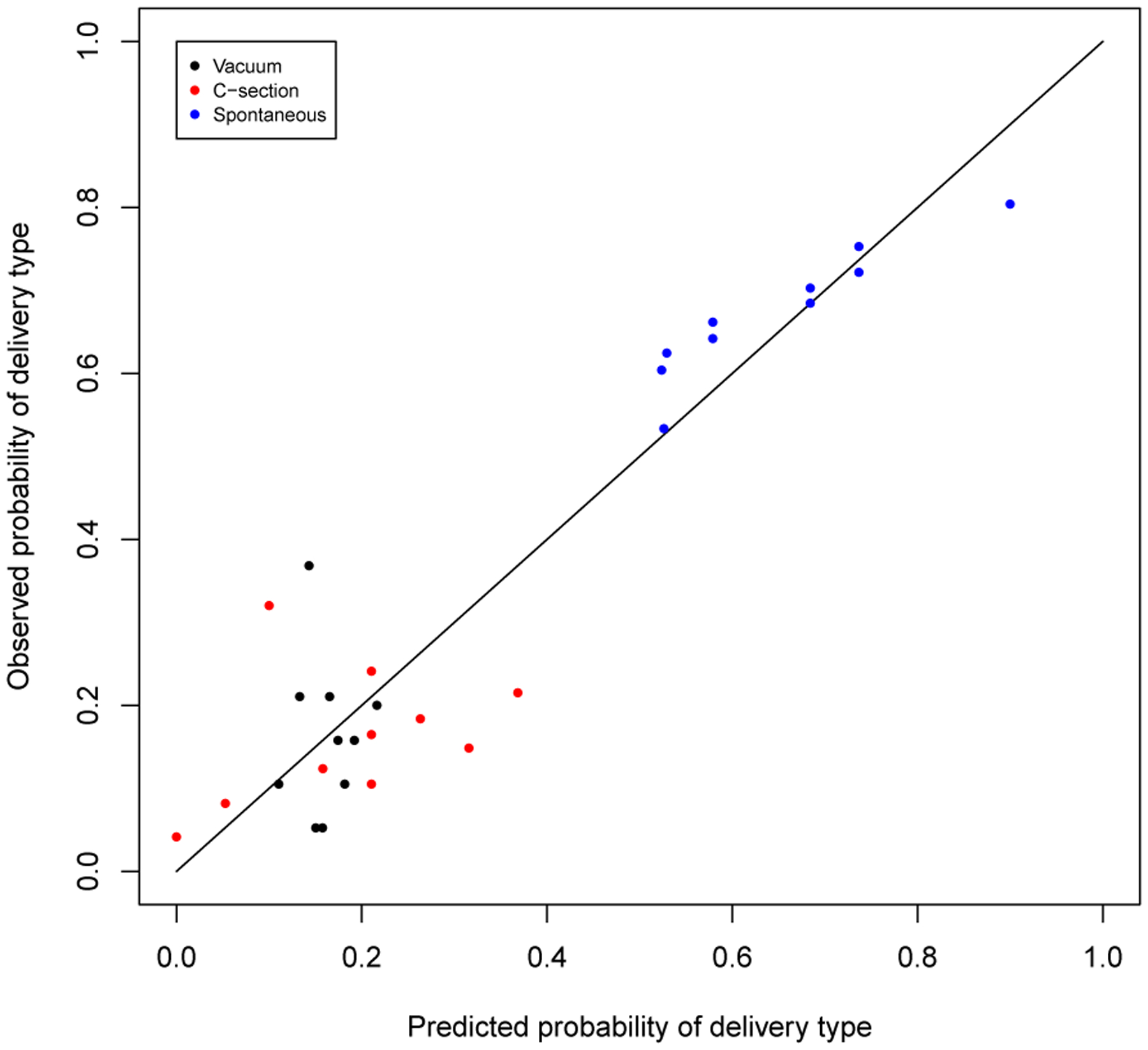
Decile plots of the predicted probability versus the corresponding observed proportions.

Figure 4:

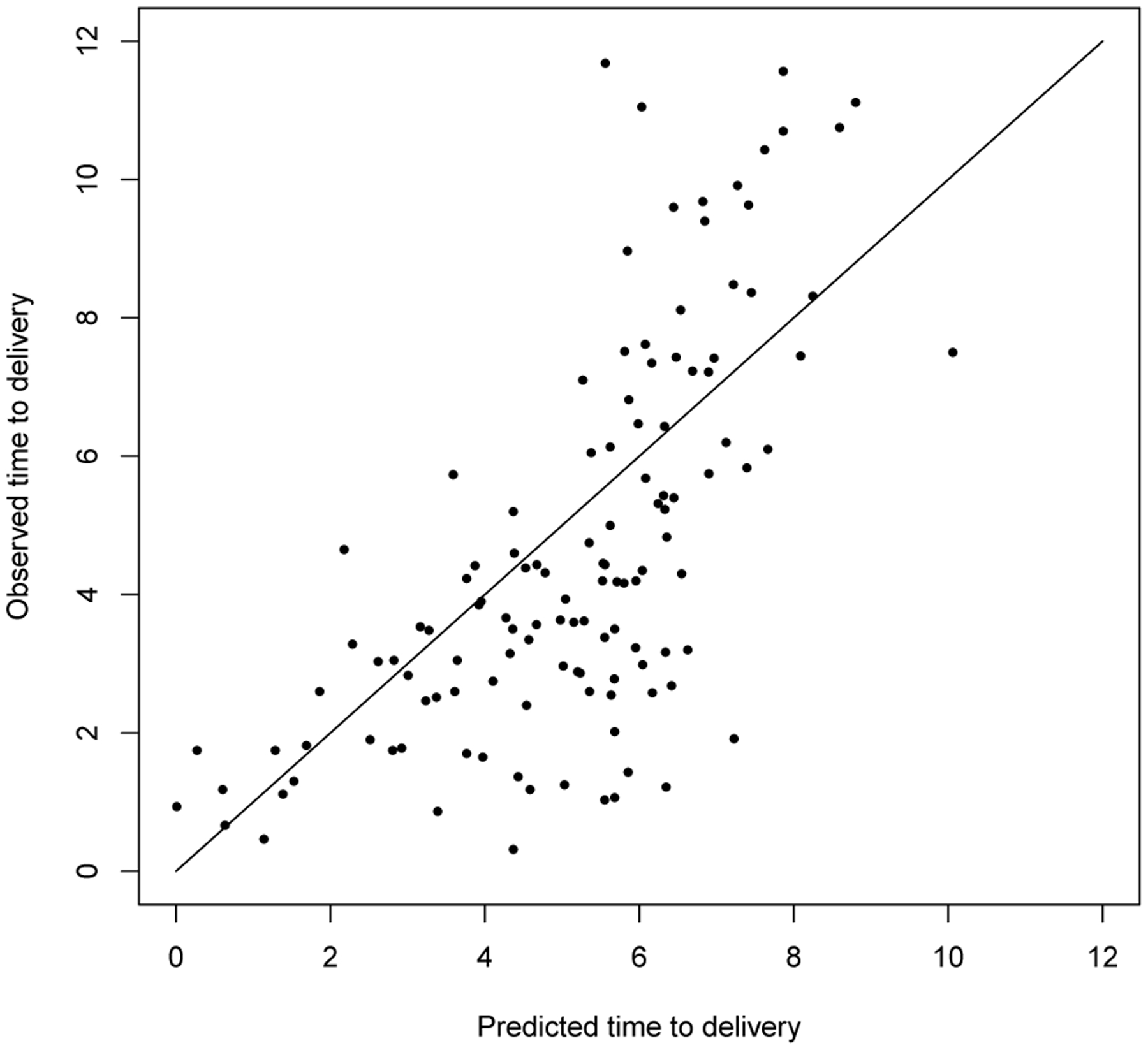
Plots of predicted time to delivery from last observed station value

6. Discussion

This article proposed a joint model of longitudinal and time-to-event data when there is no natural time zero and when there are competing risks. For the labor example, station values are measured longitudinally and the time of study entry is not a natural reference point since expecting mothers come to the hospital at different points in their late pregnancy. The competing risk aspects need to be considered since delivery type is an important component of the endpoint and time-to-delivery may be influenced by the type of delivery. The model led to important scientific observations. First, the dynamics in labor (longitudinal station process) is associated with delivery time such that the time to delivery is shorter when the velocity of station is higher. This is particularly pronounced in the later stage of labor (after the station value crosses zero). The type of delivery is also associated with station velocity. Most notably, a C-section is much more likely when the velocity (before and after a station value of zero) is delayed relative to the typical profile. This later observation is consistent with clinical experience.

For the labor progression application, the reference time (time zero) used is the time from when the station value is zero. The proposed approach allows us to use all the subjects’ data to estimate, including those who started the observation process before and after having reached time zero. In our application, we had such data. The model may be only weakly identifiable in situations where the observation process begins after a dilation value of zero. In this latter case, we recommend that the model not be used.

Although, the model is useful for understanding etiology through a close examination of the model parameters, the prediction of delivery times was not that good in some situations. Our prediction results demonstrated that prediction was accurate when the time to delivery was less than approximately 2 hours, while it was less accurate for longer range predictions. Although this is a bit disappointing, it is not surprising that a single longitudinal biomarker would be able to accurately predict delivery time among spontaneous pregnancies. The model can be extended to incorporate multiple longitudinal biomarkers in the future. Plots of the deciles of risk shows that there is a fairly large range in predictive probabilities and that the predictive model is well calibrated. Thus, the model may be very useful for predicting an individual woman’s risk of a spontaneous delivery.

The proposed modeling framework addresses the issue of relating a longitudinal biomarker to survival when there is no clearly defined time zero. Although this was motivated by a study of labor progression where women come to the hospital at different times during their labor process, the methodology would apply to any study of the effect of a disease severity score on survival where subjects are enrolled at varying levels of initial disease severity. Another example comes from studying the relationship between disability and survival in multiple sclerosis. Disease severity in multiple sclerosis is often characterized using the expanded disability status scale (EDSS) which ranges between 0 and 10 in 0.5 increments. The proposed method may be used to assess the relationship between changes in EDSS and survival in a population where subjects enroll in the study at different levels of disability.

References

- Abranowitz M and Stegun IA (1972). Handbook of mathematical functions with formulas, graphs, and mathematical tables. New York, Dover Publications, Inc. [Google Scholar]
- Celeux G, Forbes F, Robert CP, and D. M. Titterington D (2006). Deviance information criteria for missing data models. Bayesian Analysis, 1:651–674. [Google Scholar]
- Chen M-H, Dey DK, and Shao Q-M (1999). A new skewed link model for dichotomous quantal response data. Journal of the American Statistical Association, 94:1172–1186. [Google Scholar]
- Chen M-H, Shao OM, and Ibrahim JG (2000). Monte Carlo Methods in Bayesian Computation. New York, Springer-Verlag. [Google Scholar]
- Cowles C and Carlin BP (1996). Markov chain monte carlo convergence diagnostics: a comparative review. Journal of the American Statistical Association, 91:883–904. [Google Scholar]
- Hastings WK (1970). Monte carlo sampling methods using markov chains and their applications. Biometrika, 57:97–109. [Google Scholar]
- Kim S, Chen M-H, and Dey DK (2008). Flexible generalized t-link models for binary response data. Biometrika, 95:93–106. [Google Scholar]
- Liu JS (1994). The collapsed gibbs sampler in bayesian computations with applications to a gene regulation problem. Journal of the American Statistical Association, 89:958–66. [Google Scholar]
- McLain AC and Albert PS (2014). Modeling longitudinal data with a random change point and no time-zero: applications to inference and prediction of the labor curve. Biometrics, 70:1052–1060. [DOI] [PubMed] [Google Scholar]
- Rizopoulos D (2012). Joint models for longitudinal and time-to-event data: with applications in R. Boca Raton: Chapman & Hall/CRC. [Google Scholar]
- Spiegelhalter DJ, Best NG, Carlin BP, and van der Linde A (2002). Bayesian measures of model complexity and fit (with discussion). Journal of Royal Statistical Society, B, 64:583–639. [Google Scholar]