A multivariate spatio-temporal model for the incidence of imported COVID-19 cases and COVID-19 deaths in Cuba

Abstract

To monitor the COVID-19 epidemic in Cuba, data on several epidemiological indicators have been collected on a daily basis for each municipality. Studying the spatio-temporal dynamics in these indicators, and how they behave similarly, can help us better understand how COVID-19 spread across Cuba. Therefore, spatio-temporal models can be used to analyze these indicators. Univariate spatio-temporal models have been thoroughly studied, but when interest lies in studying the association between multiple outcomes, a joint model that allows for association between the spatial and temporal patterns is necessary. The purpose of our study was to develop a multivariate spatio-temporal model to study the association between the weekly number of COVID-19 deaths and the weekly number of imported COVID-19 cases in Cuba during 2021. To allow for correlation between the spatial patterns, a multivariate conditional autoregressive prior (MCAR) was used. Correlation between the temporal patterns was taken into account by using two approaches; either a multivariate random walk prior was used or a multivariate conditional autoregressive prior (MCAR) was used. All models were fitted within a Bayesian framework.

1. Introduction

In March 2020, the World Health Organisation declared the coronavirus disease (COVID-19) to be a pandemic. COVID-19 is a respiratory disease caused by an infection with the severe acute respiratory syndrome coronavirus 2 (SARS-CoV-2). On March 11, 2020, three Italian tourists in Cuba tested positive for the virus. These were the first confirmed cases in Cuba, marking this date as the beginning of the epidemic on the island (Galbán-García and Más-Bermejo, 2021). In Cuba, the largest wave of COVID-19 infections took place in 2021, peaking at the end of August 2021 (Dong et al., 2020). This wave was most likely caused by the SARS-CoV-2 Delta variant, as this variant had replaced the other variants by July 2021 and spread rapidly throughout the country (Más-Bermejo et al., 2022). In order to monitor the COVID-19 epidemic, data on several epidemiological indicators, such as the number of cases, hospitalizations and deaths are being collected at the municipal level throughout the island. The aim of this study is to evaluate the spatio-temporal trend in the number of deaths due to COVID-19 and the number of imported cases of COVID-19, as well as the association between these two indicators.

The monitoring of geographic and temporal trends in these indicators is essential to the understanding of the epidemiology of the disease throughout the region. In particular, simultaneously analyzing such trends among different indicators allows researchers to gain in-depth insight into how COVID-19 spread across the island and the extent it affected Cuba’s population and healthcare system. This is often done using spatio-temporal statistical models that take into account dependencies in space and time. Univariate spatio-temporal models have been extensively studied (see, for example, Lawson, 2021 and Haining and Li, 2020 for an overview), but models that exploit the association between the spatial and temporal patterns of multiple indicators have been studied to a lesser extent. In this article, we propose a joint model for multivariate spatio-temporal data to jointly analyze the number of imported COVID-19 cases and the number of COVID-19 related deaths across the municipalities in Cuba.

Multivariate models for two or more spatial outcomes have been studied extensively. Most of the research that has been done extended the univariate conditional autoregressive (CAR) models to the multivariate setting. The theoretical properties of multivariate Gaussian Markov Random Fields (GMRF) were first described by Mardia (1988). His work extends the work of Besag (1974). However, in his models, separable models are proposed and identical smoothing parameters for all outcomes are assumed. Non-separable Multivariate Conditional Autoregressive (MCAR) models that allow for different spatial smoothing parameters have been developed by Gelfand and Vounatsou (2003). These multivariate CAR models have been further developed by Jin et al. (2005) and Jin et al. (2007), the latter using an approach based on a linear model of coregionalization. A comprehensive review of multivariate conditional autoregressive models for multivariate spatial count data can be found in MacNab (2018).

For spatio-temporal count data, some multivariate models have been proposed recently. Lee et al. (2022) proposed a multivariate spatio-temporal correlation model. In this model, the set of spatial, temporal and spatio-temporal random effects is represented with a single set of random effects that is modeled with a zero-mean multivariate Gaussian Markov random field, and the correlation between the outcomes is captured by incorporating a between outcome covariance matrix in the precision matrix. Thus, their model does not estimate the correlation between the spatial and temporal trends separately, but captures the association between the responses by estimating one correlation parameter. Vicente et al. (2021) proposed a multivariate spatio-temporal model based on P-splines in which correlation between the coefficients of the spatial and temporal P-splines is induced. A multivariate model for spatio-temporal areal data based on M-models was recently proposed by Vicente et al. (2020).

In the joint model for multivariate spatio-temporal data that is proposed in this paper, a multivariate CAR model is used to induce correlation between spatial patterns. Correlation between temporal patterns is incorporated by using a multivariate random walk prior for the temporal random effects. We also argue that this multivariate random walk prior can be modeled with a multivariate CAR prior, since CAR priors can be used for the temporal random effects in the univariate case (Fahrmeir and Lang, 2001). To the best of our knowledge, this is the first time that a MCAR prior is used for the temporal random effects in a multivariate spatio-temporal model.

The rest of this paper is organized as follows. In Section 2, the data are described. In Section 3, we lay out the methodology and in Section 4, the results of the analyses of the number of imported COVID-19 cases and the number of COVID-19 deaths are presented. Finally, a discussion is provided in Section 5.

2. Data

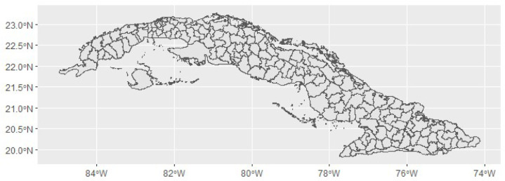
We obtained data from January 1, 2021 to October 31, 2021, given that this time period includes the largest wave of COVID-19 infections and deaths in Cuba. Beta and Delta variants circulated predominantly in the territory during this period (Guzmán et al., 2022). High-quality data are available on several COVID-19 indicators disaggregated at the municipality level, the spatial unit used in the analysis. The country is divided into 169 municipalities (Fig. 1), with an average population of 66,628 inhabitants per municipality, ranging from 10,319 to 509,841 people. Official daily COVID-19 deaths reported by the Ministry of Public Health, MINSAP, were recorded in Cuba’s national COVID-19 database. Death due to COVID-19 was defined according to the WHO definition: a person who died as a result of confirmed COVID-19, with symptoms clinically compatible with the disease (WHO, 2021). All cases confirmed by PCR testing were classified as imported or local. Daily mortality and imported case data were extracted by municipality for the study period and aggregated weekly to avoid excess null counts in the daily data and to account for weekday and weekend effects (Sahu and Böhning, 2022). Data on population size, used as an offset in the Poisson models, and population density, used as a covariate in the models, were provided by the Cuban National Statistical Office (ONE, http://www.onei.gob.cu). The latitude and longitude of the centroid and the cartographic data set with the boundaries of the municipalities were provided by the Institute of Geography.

Fig. 1.

Map of the 168 municipalities in Cuba.

3. Methodology

Let $y_{ijk}$ be the observed number of imported COVID-19 cases ($k=1$) or the observed number of COVID-19 deaths ($k=2\text{)}$ in municipality $i$ ($i=1,\dots ,I=168$) at week $j$ ($j=1,\dots ,J=44$). Instead of modeling daily data, we modeled weekly data due to the excess of zero counts in the daily data and to take into account weekday/weekend effects (Sahu and Böhning, 2022). We assume that both the number of imported COVID-19 cases and COVID-19 deaths follow a Poisson distribution with mean ${\mu }_{ijk}$ (Lawson, 2018):

$$y_{ijk}|{\mu }_{ijk}\sim \text{Pois}\left({\mu }_{ijk}\right)log\left({\mu }_{ijk}\right)=O_{ijk}+log\left({\theta }_{ijk}\right),$$

where $O_{ijk}$ is the offset and ${\theta }_{ijk}$ is the relative risk. Often, the expected counts are used as offsets. These expected counts can be obtained using indirect or direct standardization based on age and sex demographics. However, given that the appropriate data are not available for using these methods, we used the logarithm of the population size ($log\left(p_i\right)$) for the offset instead.

3.1. Univariate spatio-temporal models

First, we modeled the two outcomes separately. For this purpose, we used the spatio-temporal models suggested by Knorr-Held (2000) to model the log relative risks. In these models, the log relative risk is defined in terms of random effects:

$$log\left({\theta }_{ijk}\right)={\beta }_{0k}+{\beta }_{1k}\ast P{D}_i+u_{ik}+v_{ik}+g_{jk}+{\psi }_{ijk}\text{with}k=1,2,$$

Here, the spatial component is modeled by including a convolution $u_{ik}+v_{ik}$, where $u_{ik}$ is the correlated spatial component for outcome $k$, modeling spatially correlated heterogeneity, while spatially uncorrelated heterogeneity in outcome $k$ is modeled through $v_{ik}$. Both components are constant in time. The temporal component for each outcome is modeled by including the random effect $g_{jk}$, and a space–time interaction term is also included (${\psi }_{ijk}$). In addition, we incorporated population density (PD) in the model as a covariate. Population density is defined as the number of inhabitants per square kilometers, scaled by a factor of 100 to improve model convergence. ${\beta }_{1k}$ is the corresponding regression coefficient, and ${\beta }_{0k}$ the outcome-specific intercept.

For the spatially correlated random effects $u_k=(u_{1k},\dots ,u_{168k})$, a Gaussian intrinsic conditional autoregressive (ICAR) prior was assumed (Besag et al., 1991), which can be seen as a form of a Gaussian Markov random-field model:

$$u_k\sim N(0,{\left[{\tau }_k(D-W)\right]}^{-1})\text{with}k=1,2,$$

where the 168 × 168 matrix $D$ is diagonal with diagonal elements $m_i$ representing the number of neighbors of municipality $i$ and where $W$ is the adjacency matrix where $W_{ii}=0$, $W_{ij}=1$ if the municipalities $i$ and $j$ are adjacent, meaning that they share a common border, and $W_{ij}=0$ if the municipalities are not adjacent. This results in queen contiguity-based spatial weights. Note that since this will result in a null vector for the island Isla de la Juventud, we considered Batabano (Mayabeque) as a neighbor for the island, since Isla de la Juventud is connected by ferries to this municipality. We will denote this ICAR prior with $u_{ik}\sim ICAR\left({\tau }_{u_k}^{-1}\right)$, where $\tau$ corresponds to the precision (inverse variance) parameter. For the uncorrelated spatial random effects, $v_{ik}$, an independent zero-mean Gaussian prior distribution was assumed: $v_{ik}\sim N(0,{\tau }_{v_k}^{-1})$ (Besag et al., 1991, Lawson, 2018, Jin et al., 2007).

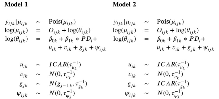
For the temporal main effect $g_{jk}$, a type of temporal random walk of order one (RW(1)) was assumed. Two implementation approaches were considered. In the first approach (Model 1), the RW(1) prior was implemented with a Gaussian prior distribution: $g_{jk}\sim N(g_{j-1,k},{\tau }_{g_k}^{-1})$ (Lawson, 2021). In a second approach (Model 2), we implemented the RW(1) prior with a one-dimensional ICAR prior: $g_{jk}\sim ICAR\left({\tau }_{g_k}^{-1}\right)$. Indeed, it has been shown that the intrinsic CAR distribution is equivalent to a Gaussian random walk in one dimension when the temporal adjacency matrix $Q$ is appropriately specified (Fahrmeir and Lang, 2001, Thomas et al., 2004). Let $Q_{hl}$ denote the entries of the temporal adjacency matrix. Then $Q_{hl}=1$ if the two time points $h$ and $l$ are adjacent and $Q_{hl}=0$ if the two time points $h$ and $l$ are not adjacent. The type of RW(1) prior that is implemented with the ICAR prior can be written as

$$g_{jk}\sim N(g_{j+1,k},{\tau }_{g_k}^{-1})\text{for}j=1$$

$$g_{jk}\sim N((g_{j-1,k}+g_{j+1,k})/2,{\tau }_{g_k}^{-1}/2)\text{for}j=2,\dots ,J-1$$

$$g_{jk}\sim N(g_{j-1,k},{\tau }_{g_k}^{-1})\text{for}j=J.$$

Knorr-Held (2000) proposed four types of prior distributions for the space–time interaction term ${\psi }_{ijk}$. In our model, a Type I interaction was assumed by using an independent zero-mean Gaussian prior distribution: ${\psi }_{ijk}\sim N(0,{\tau }_{{\psi }_{ijk}}^{-1})$, because of the complexity of the multivariate model that we fitted in a next step.

Finally, the two responses ($k=1,2$) were each modeled separately using the following two models:

(1)

3.2. Multivariate spatio-temporal models

When interest lies in studying the association between the spatial trends and the temporal trends of the two responses, a joint model for multivariate spatio-temporal data is necessary. Just as in the univariate models, we assumed that both outcomes can be modeled with a Poisson distribution where the log relative risk is modeled with a set of spatial and temporal random effects:

Here, the random effects $u_{ik}$ and $v_{ik}$ are again the correlated and uncorrelated spatial components, respectively, $g_{jk}$ is the temporal component and ${\psi }_{ijk}$ is the space–time interaction. However, unlike in the univariate models, we allow for correlation between the spatially structured random effects and the temporal components by assuming a multivariate distribution for $u_{i1}$ and $u_{i2}$ and for $g_{j1}$ and $g_{j2}$, respectively.

For the spatially structured random effects, a multivariate extension of the univariate CAR prior has been developed by Gelfand and Vounatsou (2003). Jin et al., 2007, Jin et al., 2005 further developed these so-called multivariate CAR (MCAR) distributions. Here, we focus on the multivariate Intrinsic CAR model (MICAR). In the approach proposed by Gelfand and Vounatsou (2003), a joint distribution is assumed for the set of spatially structured effects, $u={(u_1^{\prime },u_2^{\prime })}^{\prime }$, where $u_1={(u_{11},\dots ,u_{I1})}^{\prime }$ and $u_2={(u_{12},\dots ,u_{I2})}^{\prime }$

$$u\sim N(0,{[{\Lambda }_u\otimes (D-W)]}^{-1})$$

in which ${\Lambda }_u$ is the 2 × 2 non-spatial positive definite precision matrix between the two outcomes, and the matrices $D$ and $W$ are defined as in Section 3.1. Note that $(D-W)$ is the kernel of the spatial univariate ICAR model (Lawson, 2021). Thus, the precision matrix is the Kronecker product of ${\Lambda }_u$ and the univariate ICAR form (Jin et al., 2005). In the remainder of this paper, we denoted this prior as $u_{ik}\sim MCAR(1,{\Lambda }_u)$.

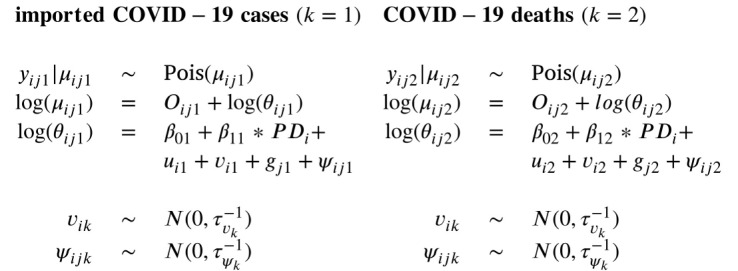
For the implementation of the temporal random effects, we propose two different approaches. In the first approach (Model 3), a multivariate extension of the RW(1) prior as implemented in Model 1 is proposed by specifying a joint multivariate Gaussian distribution for two temporal random effects:

$$\left(\begin{array}{c}\hfill g_{j1}\hfill \\ \hfill g_{j2}\hfill \end{array}\right)\sim N\left(\left(\begin{array}{c}\hfill g_{j-1,1}\hfill \\ \hfill g_{j-1,2}\hfill \end{array}\right),{\Sigma }_g\right).$$

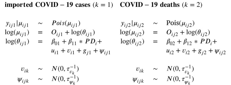
The correlation of the two random effects can then be derived from the variance–covariance matrix ${\Sigma }_g$. However, as shown in Model 2 in Section 3.1, in a univariate model, a RW(1) prior can also be implemented by using an ICAR prior for the temporal random effects. Therefore, in the second approach (Model 4), the temporal random effects of the two outcomes were modeled jointly by using the multivariate extension of the ICAR prior, $g_{jk}\sim MCAR(1,{\Lambda }_g)$, where $MCAR(1,{\Lambda }_g)$ is defined as $N(0,{[{\Lambda }_g\otimes (D_g-Q)]}^{-1})$, like for the spatially structured effects. Only now, ${\Lambda }_g$ is the 2 × 2 non-temporal precision matrix for the two outcomes, $D_g$ is a diagonal matrix where the diagonal elements are the number of adjacent time points, and $Q$ is the temporal adjacency matrix.

The spatially unstructured random effects, $v_{i1}$ and $v_{i2}$, and the space–time interactions, ${\psi }_{ij1}$ and ${\psi }_{ij2}$, were modeled separately using the same priors as in the univariate models (as in (1)). In summary, the following two multivariate models were fitted to study the spatial and temporal associations between the two outcomes:

$$\underset{\_}{\mathbf{Model\; 3}}$$

(2)

$$\left(\begin{array}{c}\hfill g_{j1}\hfill \\ \hfill g_{j2}\hfill \end{array}\right)\sim N\left(\left(\begin{array}{c}\hfill g_{j-1,1}\hfill \\ \hfill g_{j-1,2}\hfill \end{array}\right),{\Sigma }_g\right)$$

$$u_{ik}\sim MCAR(1,{\Lambda }_u)$$

$$\underset{\_}{\mathbf{Model\; 4}}$$

(3)

$$g_{jk}\sim MCAR(1,{\Lambda }_g)$$

$$u_{ik}\sim MCAR(1,{\Lambda }_u)$$

3.3. Model implementation

All models were fitted within the Bayesian framework, in which Markov chain Monte Carlo (MCMC) methods are used to approximate the posterior distributions. The MCMC methods were performed using the NIMBLE package, version 0.12.2 (de Valpine et al., 2017), in R 4.2.0 (R Core Team, 2022). We ran four chains of 1,100,000 iterations each. The first 100,000 iterations of each chain were discarded as burn-in period, and a thinning factor of 1000 was used. The reason for this high thinning factor and these long chains is the high autocorrelation in the MCMC samples for the intercept parameters in Models 1 and 3. The remaining posterior samples were summarized by the posterior means, standard deviations and 95% equal-tailed credible intervals. Trace plots, effective sample size (ESS) and the Potential Scale Reduction factors ($\hat{R}$) were examined to assess convergence (Gelman and Rubin, 1992). Convergence was assumed since all $\hat{R}$ values were below 1.1. Different models were compared using the well known Watanabe–Akaike information criterion (WAIC) (Watanabe and Opper, 2010) and the mean squared predictive error (MSPE) defined as

$$MSP{E}_k=\sum _{ij}\frac{{(y_{ijk}-{\hat{y}}_{ijk})}^2}{n}$$

(Lawson et al., 2017). All data and code used in this study are openly available on Github: https://github.com/DriesDWitte/Multivariate_Spatio_Temporal_Model.

3.3.1. Prior distributions

Non-informative prior distributions were assumed. Flat prior distributions were provided for the regression coefficients of the intercepts ${\beta }_{01}$ and ${\beta }_{02}$. For all standard deviations (${\sigma }_{{\beta }_{0k}}$, ${\sigma }_{u_k}$, ${\sigma }_{v_k}$, ${\sigma }_{g_k}$, ${\sigma }_{{\psi }_k}$), defined in terms of the precision as $\sigma ={\tau }^{-1/2}$, a uniform distribution was assumed over the range (0,10) (Gelman, 2006, Lawson et al., 2017). In NIMBLE, the ICAR prior is implemented as the dcar_normal distribution. The MVCAR, however, is not directly implemented in NIMBLE, but it is possible to fit this model using the linear model of co-regionalization (LMC) approach of Jin et al. (2007). Code to fit the MVCAR model in NIMBLE is provided by Lawson (2021). Inverse-Wishart priors were assigned to ${\Lambda }_g$ and ${\Lambda }_u$ with two degrees of freedom and a 2 × 2 identity matrix as scale matrix.

3.3.2. Sensitivity analyses

The impact of the assumed priors was examined through a sensitivity analysis where the regression coefficients were given a Normal prior distribution with zero mean and a small precision of 0.001, and where the inverse-gamma(0.001,0.001) prior distribution was assumed for the variance parameters. We compared the resulting posterior distributions and found no noticeable impact of the choice of prior distribution on the posterior distributions of the parameters. Our overall conclusions remained intact. In a second sensitivity analysis, a distance-based neighborhood structure, where the k nearest municipalities are chosen as neighbors, was considered to study the robustness of our results, with $k=4$. The different neighborhood structures are given in Figure .9 in the Supplemental Materials. The results remained very similar regardless of the neighborhood structure used, and the choice of neighborhood structure did not affect our findings and conclusions.

4. Results

4.1. Exploratory data analysis

Before fitting the models, we explored the data by means of summary statistics and graphical displays. For this purpose, we compared the number of deaths per 10,000 people and the number of imported cases per 10,000 people across the different municipalities. For the number of deaths, this rate ranges from 0 to 7.0991, with a mean value of 0.1638. The mean value for the rate of imported cases is 0.1340 and ranges from 0 to 15.8748. The median was zero for both rates. The average rate of death and rate of imported cases across all weeks for each municipality is plotted in Fig. 2. The average number of deaths per 10,000 inhabitants was the largest for Caimanera (0.5647), followed by Moron (0.5215) and San Cristobal (0.4752). For the average number of imported cases per 10,000 inhabitants, we observed the largest value for Moron (1.6129), followed by Cardenas (1.1499) and Holguin (0.4909). To explore the temporal trend of the two rates, we plotted the rates for the 44 weeks in our study for each municipality separately in Fig. 3.

Fig. 2.

Average rate across all weeks for each municipality.

Fig. 3.

Temporal trend of the rates for the 44 weeks for each municipality separately.

4.2. Results of the univariate models

After exploring the data, we started with analyzing the two outcomes separately by fitting the two models described in (1).

4.2.1. Deaths

We begin by describing the results of the fitted models for the number of deaths. The parameter estimates from Models 1 and 2 are presented in Table 1. The population density was not found to be associated with the number of deaths, as the 95% CI contains zero in both models. For Model 1, the value of the WAIC is equal to 12980.21 and the MSPE is equal to 2.1918 [1.9836; 2.4284]. The WAIC and the MSPE are, respectively, 12986.22 and 2.1942 [1.9757; 2.4398] for Model 2. Both the WAIC and the MSPE are smaller for Model 1, but since the difference is so small, one may argue that both models are equally supported by the data.

Table 1.

Parameter estimates of the univariate models for the number of deaths.

	Mean	SD	95%CI
Model 1
${\beta }_{01}$	−14.4053	0.5427	[−15.4949; −13.3136]
${\beta }_{11}$	0.0019	0.0011	[−0.0002; 0.0039]
${\sigma }_{v_1}$	0.1684	0.0816	[0.0101; 0.3135]
${\sigma }_{u_1}$	0.5011	0.1057	[0.2875; 0.6979]
${\sigma }_{g_1}$	0.3658	0.0515	[0.2781; 0.4759]
${\sigma }_{{\psi }_1}$	0.9412	0.0232	[0.8964; 0.9885]
Model 2
${\beta }_{01}$	−12.3517	0.0374	[−12.426; −12.2794]
${\beta }_{11}$	0.0019	0.0011	[−0.0002; 0.0042]
${\sigma }_{v_1}$	0.1959	0.0677	[0.0509; 0.3202]
${\sigma }_{u_1}$	0.4831	0.0973	[0.2910; 0.6719]
${\sigma }_{g_1}$	0.3632	0.0505	[0.2786; 0.4770]
${\sigma }_{{\psi }_1}$	0.9404	0.0232	[0.8951; 0.9867]

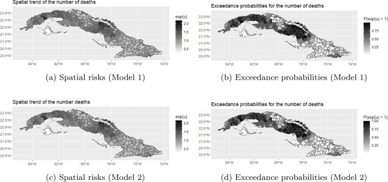
To explore the spatial trend, we plotted the posterior mean of the municipality-specific spatial risks, calculated as $exp\left(u_{i1}\right)$, together with the exceedance probabilities, calculated as $P(exp\left(u_{i1}\right)>1)$, for both models in Fig. 4. The exceedance probabilities can be used to detect municipalities that have an elevated risk. The plots give identical results for Models 1 and 2. From these plots, we noticed that the largest exceedance probabilities can be observed in the middle and Northern part of Cuba. The municipality with the largest estimated posterior mean is Centro Habana, a densely populated area in Ciudad de La Habana (Havana City), followed by Moron (Ciego de Avila), a municipality with a direct connection to the touristic Keys in northern Cuba and Chambas (Ciego de Avila).

Fig. 4.

Posterior means of the spatial risks and exceedance probabilities for the number of deaths.

The global temporal evolution of the number of deaths can be explored by looking at the posterior means of $exp\left(g_{j1}\right)$. These are displayed in Fig. 5 together with the 95% credible intervals. The shape of the global temporal trend is the same for both models. The trend shows that the number of deaths starts to increase from week 25 onwards and reaches its peak at week 36.

Fig. 5.

Posterior means of the temporal risks for the number of deaths.

4.2.2. Imported cases

The parameter estimates from the fitted models for the number of imported cases are given in Table 2. Also for the number of imported cases, the density of the population was not found to have a significant effect. The lowest value for the WAIC and MSPE is observed for Model 2; the value of the WAIC for Model 1 was equal to 13599.17, for Model 2 it was equal to 13598.48. The MSPE was equal to 2.4757 [2.2008; 2.8284] for Model 1 and 2.4734 [2.1998; 2.8236] for Model 2. However, the difference is again negligible, suggesting that the two models fit equally well.

Table 2.

Parameter estimates of the univariate models for the number of imported cases.

	Mean	SD	95%CI
Model 1
${\beta }_{02}$	−10.6861	0.3568	[−11.2998; −9.9751]
${\beta }_{02}$	0.0034	0.0019	[−0.0002; 0.0072]
${\sigma }_{v_2}$	0.5437	0.0802	[0.3630; 0.6857]
${\sigma }_{u_2}$	0.6693	0.1860	[0.3495; 1.0829]
${\sigma }_{g_2}$	0.3557	0.0465	[0.2776; 0.4594]
${\sigma }_{{\psi }_2}$	0.9097	0.0242	[0.8626; 0.9582]
Model 2
${\beta }_{02}$	−12.2026	0.0549	[−12.3152; −12.1019]
${\beta }_{12}$	0.0034	0.0019	[−0.0005; 0.0070]
${\sigma }_{v_2}$	0.5408	0.0853	[0.3480; 0.6911]
${\sigma }_{u_2}$	0.6809	0.1995	[0.3439; 1.1359]
${\sigma }_{g_2}$	0.3563	0.0470	[0.2752; 0.4590]
${\sigma }_{{\psi }_2}$	0.9099	0.0241	[0.8629; 0.9589]

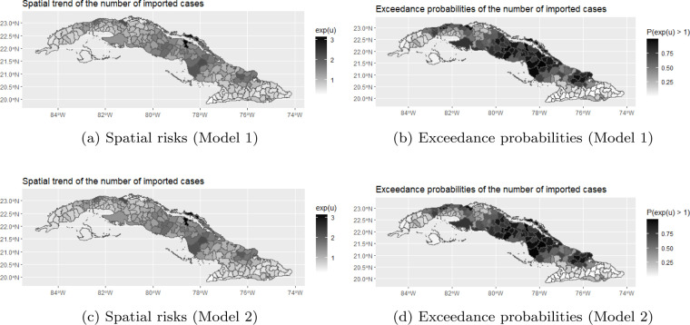
We explored the spatial trend by plotting the posterior mean of the municipality-specific spatial risks ($exp\left(u_{i2}\right)$) and the exceedance probabilities ($Pexp(u_{i2}>1)$) for both models (Fig. 6). Again, these plots are identical for both models. They show large exceedance probabilities in the middle part of the country and in the area of Ciudad de La Habana. The largest estimated posterior mean of the spatial risks was observed for Moron (Ciego de Avila). The second and third largest posterior mean of the spatial risks was observed for Plaza De La Revolución (Ciudad de La Habana) and Playa (Ciudad de La Habana), respectively.

Fig. 6.

Posterior means of the spatial risks and exceedance probabilities for the number of imported cases.

We also studied the global temporal evolution of the number of imported cases. For this purpose, the posterior means of $exp\left(g_{j2}\right)$ and the 95% credible intervals are displayed in Fig. 7. Again, we noticed that the shape of the estimated trend is the same for both models. The number of imported cases seems to increase from week 11 onwards, reaching a first peak in week 20. After that, it decreases again until week 22. A second peak in the temporal trend of the number of imported cases was observed in week 26.

Fig. 7.

Posterior means of the temporal risks for the number of imported cases.

4.3. Results of the multivariate models

After modeling the two outcomes univariately, we fitted the two models described in (2) and in (3). These models were fitted using different time lags for the number of deaths. Indeed, the number of deaths might be affected by the number of imported cases in the previous weeks.

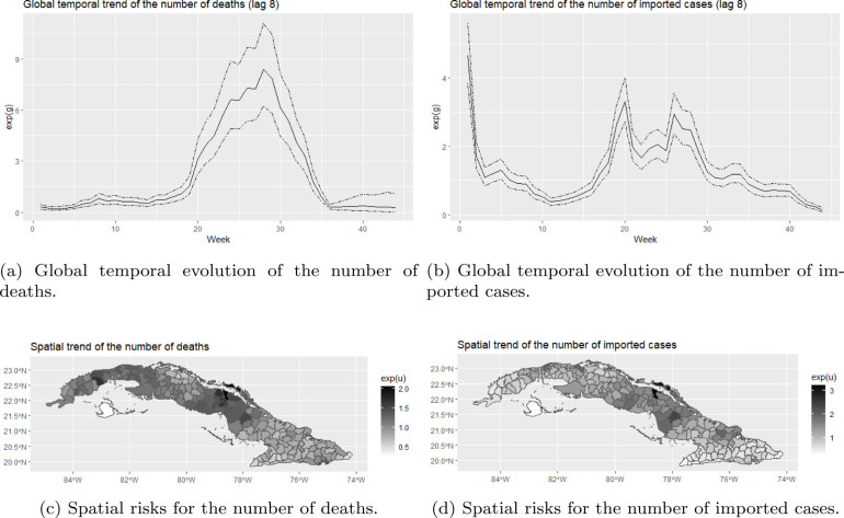
The results of Models 3 and 4 are summarized in Table 3. In this table, the WAIC, MSPE and the temporal and spatial correlations are given. The results of Model 3 and the results of Model 4 are similar, again indicating that the two models give an equally good fit. The correlation between the temporal random effects $g_{j1}$ and $g_{j2}$ was not significant for any of the time lags, indicating that there might be some events happening in time that affect both outcomes differently. The estimated global temporal evolution for Model 4 with a time lag of 8 weeks are displayed in Fig. 8, since for this time lag the temporal correlation was the highest. We chose to display the results of Model 4 since the MSPEs were smaller. However, the results of Model 3 with a time lag of 8 weeks are also plotted in Figure .11 in the Supplemental Materials. As expected, the global temporal evolution from the multivariate models are identical to the global temporal evolutions from the univariate models.

Table 3.

Summary of the results of Model 3 and Model 4.

Lag	WAIC	MSPE Deaths	MSPE Imported Cases	Temporal correlation	Spatial correlation
Model 3
2	26 442.78	2.1997 [1.9891; 2.4440]	2.4753 [2.1965; 2.8290]	0.1147 [−0.2425; 0.4474]	0.3775 [0.1186; 0.6325]
4	26 269.23	2.2102 [1.9974; 2.4697]	2.4725 [2.1983; 2.8405]	−0.0642 [−0.4096; 0.3058]	0.3648 [0.0998; 0.6328]
6	26 062.67	2.2163 [1.9972; 2.4708]	2.4702 [2.1995; 2.8344]	0.0406 [−0.3109; 0.3839]	0.3592 [0.0882; 0.6219]
8	25 846.76	2.2159 [1.9869; 2.5168]	2.4771 [2.2017; 2.8510]	0.2322 [−0.1187; 0.5424]	0.3477 [0.0773; 0.6155]
10	25 645.08	2.2278 [1.9808; 2.5662]	2.4721 [2.2088; 2.8562]	0.1248 [−0.2329; 0.4568]	0.3358 [0.0606; 0.6158]
12	25 463.83	2.2479 [1.9856; 2.6932]	2.4765 [2.2072; 2.8479]	0.0728 [−0.2821; 0.4124]	0.3229 [0.0448; 0.6077]
Model 4
2	26 445.24	2.1981 [1.9893; 2.4410]	2.4701 [2.2069; 2.8387]	0.1371 [−0.2779; 0.5163]	0.3651 [0.1061;0.6121]
4	26 272.15	2.2127 [1.9886; 2.4725]	2.4730 [2.1994; 2.8401]	−0.0668 [−0.4554; 0.3783]	0.3622 [0.1025; 0.6244]
6	26 069.91	2.2169 [1.9970; 2.4850]	2.4779 [2.1980; 2.8460]	0.0574 [−0.3708; 0.4900]	0.3560 [0.0865;0.6255]
8	25 847.91	2.2067 [1.9821; 2.4779]	2.4709 [2.1985; 2.8353]	0.2702 [−0.1539; 0.6102]	0.3392 [0.0766; 0.6034]
10	25 644.45	2.2745 [1.9846; 2.5830]	2.4766 [2.2052; 2.8361]	0.1679 [−0.3355; 0.5884]	0.3201 [0.0548; 0.6024]
12	25 461.79	2.2327 [1.9794; 2.6048]	2.4735 [2.1984; 2.8383]	0.1295 [−0.3514; 0.5524]	0.3006 [0.0316; 0.5846]

Fig. 8.

Global temporal trends and spatial trends for the number of deaths and imported cases from Model 4.

A positive and significant correlation was found between the spatially structured random effects, $u_{i1}$ and $u_{i2}$, in all models for all time lags. In Figure 8 and Figure .11, we also plotted the posterior means of the municipality-specific spatial risks for Model 4 and Model 3, respectively. For both the number of deaths and the number of imported cases, we observe larger spatial risks in the middle part of Cuba and in the area of Ciudad de La Habana, and smaller spatial risks in the Southern part of the country. Especially for Moron, we notice a large spatial risk for the number of imported cases and for the number of deaths as well.

5. Discussion

In this paper, the numbers of imported cases and deaths due to COVID-19 were analyzed across the 168 municipalities of Cuba using spatio-temporal models. First, we analyzed the two outcomes univariately using two models (Models 1 and 2). Both models give similar results and lead to the same conclusions regarding the spatial patterns and the temporal evolutions. For the number of deaths, the spatial pattern shows higher spatial risks in the middle and Northern parts of Cuba. This is possibly because the center of the country and some municipalities of Havana have the highest aging population, with the highest risk of death. For the number of imported cases, the spatial pattern also shows higher spatial risks in the middle part of Cuba and in the area of Ciudad de La Habana. The highest spatial risks of imported cases are observed in Moron, Cardenas and Holguín. These municipalities are close to or are tourist attractions. The global temporal trend for the number of imported cases shows two peaks; one in week 20 and another in week 26. The peak in the global temporal trend for the number of deaths is in week 36.

We did not find a significant effect of population density on the number of deaths or the number of imported cases. While this may seem counterintuitive, there are several possible explanations. For example, it is possible that the effect of population density is non-linear. Second, it is likely that the number of people passing through a municipality, rather than population density, affects the number of deaths and imported cases. For Moron, we observed a high relative risk for both outcomes, although this is a municipality with a relatively low population density (56.6350 persons per square kilometer). A third possibility is that the effect of population density on the incidence of deaths or imported cases depends on whether the population density exceeds a certain threshold. Further research is needed to investigate these hypotheses.

The main goal of this article was to develop and present methodology to model multiple spatio-temporal outcomes jointly, and to use this methodology to study the association between the number of deaths and imported cases. Presumably, this is the first study that investigates the spatial and temporal association between these two indicators. For this purpose, we developed two models (Model 3 and 4). As far as the authors are aware, this is the first time that an MCAR prior is used for the temporal random effects. We also fitted these models for different time lags. The results of the two joint models are again similar. The analyses reveal a positive and significant correlation between the spatial patterns of the number of deaths and imported cases, with higher spatial risks in the center of Cuba and lower spatial risks in the South. This might indicate that there are some common underlying spatial risk factors affecting both the number of deaths and imported cases (e.g., demographic or socio-economic characteristics). Specifically for Moron, we observe a high spatial risk for both the number of deaths and imported cases. Arguably, this is because Moron is the city closest to the Cayos, a group of islands very popular among tourists, with many tourists passing through or staying in Moron. Also, Moron is a municipality with a direct connection to the touristic Keys in northern Cuba and Chambas (Ciego de Avila). Furthermore, there was no significant correlation between the temporal evolutions, indicating that there may be some temporal events affecting the two outcomes differently. For instance, changes in policies regarding international travel restrictions may primarily affect the number of imported cases. The international travel restriction level in Cuba throughout the study period is displayed in Figure .10 in the Supplemental Materials (Hale et al., 2021). In addition, the vaccination campaign in Cuba started in May but was scaled at different times across the country. The temporal evolution of vaccination might also be a temporal event that affects both outcomes differentially. The immunity acquired by vaccination protected the population from the effect of transmission by infected travelers. Other temporal events that might affect the two outcomes differently are the transmissibility and severity of the circulating variants. Several variants circulated in the country in 2021 (Guzmán et al., 2022). Until July, the Beta variant was predominant, while Delta dominated for the remainder of the period.

In further research, possible extensions of the proposed models could be explored. For instance, instead of using a multivariate extension of the ICAR prior for the spatially structured random effects, one might consider using a multivariate proper CAR model. For the temporal random effects, it is, for instance, possible to assume a random walk prior of order 2 instead of order 1. Another possible extension is to also allow for correlation between the spatially unstructured effects by assuming a multivariate Gaussian prior for these random effects. In our models, we always assumed independent Gaussian priors for the space–time interactions. Different forms proposed by Knorr-Held (2000) for these interactions might also be considered. Also, another interesting extension would be to fit models that do not assume spatial stationarity since spatial variation might itself change through space.

Lastly, efforts are needed to determine factors that contribute to the excess mortality risk that is observed in some regions. In additional research, potential spatial risk factors could be identified that affect both outcomes and that may explain the positive and significant spatial correlation between imported cases and deaths. This correlation reaffirms and alerts health authorities to the importance of surveillance measures and early warning systems in regions with the highest influx of travelers. Deaths may be related to imported cases at the beginning of transmission, but once transmission is established in the country, it depends more on sociodemographic aspects and the capacity of health services to detect cases early and treat them appropriately. Cuba’s National Health System is based on equitable primary care and allocates the greatest resources to the regions in the lowest socioeconomic stratum. These regions are typically also the regions with the highest risks (Mas Bermejo et al., 2021).

Declaration of Competing Interest

The authors declare that they have no known competing financial interests or personal relationships that could have appeared to influence the work reported in this paper.

Appendix A. Supplementary data

The following is the Supplementary material related to this article.

MMC S1

.

Data availability

All data and code used in this study are openly available on Github https://github.com/DriesDWitte/Multivariate_Spatio_Temporal_Model.

References

- Besag J. Spatial interaction and the statistical analysis of lattice systems. J. R. Stat. Soc. Ser. B Stat. Methodol. 1974;36(2):192–225. [Google Scholar]
- Besag J., York J., Mollié A. Bayesian image restoration, with two applications in spatial statistics. Ann. Inst. Statist. Math. 1991;43(1):1–20. [Google Scholar]
- de Valpine P., Turek D., Paciorek C., Anderson-Bergman C., Temple Lang D., Bodik R. Programming with models: writing statistical algorithms for general model structures with NIMBLE. J. Comput. Graph. Statist. 2017;26:403–413. doi: 10.1080/10618600.2016.1172487. [DOI] [Google Scholar]
- Dong E., Du H., Gardner L. An interactive web-based dashboard to track COVID-19 in real time. Lancet Infect. Dis. 2020;20(5):533–534. doi: 10.1016/S1473-3099(20)30120-1. [DOI] [PMC free article] [PubMed] [Google Scholar]
- Fahrmeir L., Lang S. Bayesian inference for generalized additive mixed models based on Markov random field priors. J. R. Stat. Soc. Ser. C. Appl. Stat. 2001;50(2):201–220. [Google Scholar]
- Galbán-García E., Más-Bermejo P. COVID-19 in Cuba: assessing the national response. MEDICC Rev. 2021;22:29–34. doi: 10.37757/MR2020.V22.N4.5. [DOI] [PubMed] [Google Scholar]
- Gelfand A.E., Vounatsou P. Proper multivariate conditional autoregressive models for spatial data analysis. Biostatistics. 2003;4(1):11–15. doi: 10.1093/biostatistics/4.1.11. [DOI] [PubMed] [Google Scholar]
- Gelman A. Prior distributions for variance parameters in hierarchical models (comment on article by Browne and Draper) Bayesian Anal. 2006;1(3):515–534. [Google Scholar]
- Gelman A., Rubin D.B. Inference from iterative simulation using multiple sequences. Statist. Sci. 1992:457–472. [Google Scholar]
- Guzmán M.G., Pérez L., Tejero Y., Mederos D., Aguado M.E., Pintos Y., Valdes O., Álvarez M., de León L.d.R.P., Baldoquín W., et al. Emergence and evolution of SARS-CoV-2 genetic variants during the Cuban epidemic. J. Clin. Virol. Plus. 2022;2(4) doi: 10.1016/j.jcvp.2022.100104. [DOI] [PMC free article] [PubMed] [Google Scholar]
- Haining R.P., Li G. first ed. Chapman and Hall/CRC; 2020. Modelling Spatial and Spatial-Temporal Data: A Bayesian Approach. [Google Scholar]
- Hale T., Angrist N., Goldszmidt R., Kira B., Petherick A., Phillips T., Webster S., Cameron-Blake E., Hallas L., Majumdar S., et al. A global panel database of pandemic policies (Oxford COVID-19 government response tracker) Nat. Hum. Behav. 2021;5(4):529–538. doi: 10.1038/s41562-021-01079-8. [DOI] [PubMed] [Google Scholar]
- Jin X., Banerjee S., Carlin B.P. Order-free co-regionalized areal data models with application to multiple-disease mapping. J. R. Stat. Soc. Ser. B Stat. Methodol. 2007;69(5):817–838. doi: 10.1111/j.1467-9868.2007.00612.x. [DOI] [PMC free article] [PubMed] [Google Scholar]
- Jin X., Carlin B.P., Banerjee S. Generalized hierarchical multivariate CAR models for areal data. Biometrics. 2005;61(4):950–961. doi: 10.1111/j.1541-0420.2005.00359.x. [DOI] [PubMed] [Google Scholar]
- Knorr-Held L. Bayesian modelling of inseparable space-time variation in disease risk. Stat. Med. 2000;19(17–18):2555–2567. doi: 10.1002/1097-0258(20000915/30)19:17/18<2555::aid-sim587>3.0.co;2-#. [DOI] [PubMed] [Google Scholar]
- Lawson A.B. Chapman and Hall/CRC; 2018. Bayesian Disease Mapping: Hierarchical Modeling in Spatial Epidemiology. [Google Scholar]
- Lawson A.B. CRC Press; 2021. Using R for Bayesian Spatial and Spatio-Temporal Health Modeling. [Google Scholar]
- Lawson A.B., Carroll R., Faes C., Kirby R.S., Aregay M., Watjou K. Spatiotemporal multivariate mixture models for Bayesian model selection in disease mapping. Environmetrics. 2017;28(8) doi: 10.1002/env.2465. [DOI] [PMC free article] [PubMed] [Google Scholar]
- Lee D., Robertson C., Marques D. Quantifying the small-area spatio-temporal dynamics of the Covid-19 pandemic in Scotland during a period with limited testing capacity. Spatial Stat. 2022;49 doi: 10.1016/j.spasta.2021.100508. [DOI] [PMC free article] [PubMed] [Google Scholar]
- MacNab Y.C. Some recent work on multivariate Gaussian Markov random fields. Test. 2018;27(3):497–541. [Google Scholar]
- Mardia K. Multi-dimensional multivariate Gaussian Markov random fields with application to image processing. J. Multivariate Anal. 1988;24(2):265–284. [Google Scholar]
- Más-Bermejo P.I., Dickinson-Meneses F.O., Almenares-Rodríguez K., Sánchez-Valdés L., Guinovart-Díaz R., Vidal-Ledo M., Galbán-García E., Olivera-Nodarse Y., Morgado-Vega I., Dueñas-Carrera S., et al. Cuban Abdala vaccine: Effectiveness in preventing severe disease and death from COVID-19 in Havana, Cuba; A cohort study. Lancet Reg. Health-Am. 2022;16 doi: 10.1016/j.lana.2022.100366. [DOI] [PMC free article] [PubMed] [Google Scholar]
- Mas Bermejo P., Sánchez Valdés L., Somarriba López L., Valdivia Onega N.C., Vidal Ledo M.J., Alfonso Sánchez I., Seuc Jo A., Almeida Cruz Y., Morales Ojeda R. Equity and the Cuban national health system’s response to COVID-19. Revista Panam. Salud Pública. 2021;45 doi: 10.26633/RPSP.2021.80. [DOI] [PMC free article] [PubMed] [Google Scholar]
- R Core Team P. R Foundation for Statistical Computing; Vienna, Austria: 2022. R: A Language and Environment for Statistical Computing. URL https://www.R-project.org/ [Google Scholar]
- Sahu S.K., Böhning D. Bayesian spatio-temporal joint disease mapping of Covid-19 cases and deaths in local authorities of England. Spatial Stat. 2022;49 doi: 10.1016/j.spasta.2021.100519. [DOI] [PMC free article] [PubMed] [Google Scholar]
- Thomas A., Best N., Lunn D., Arnold R., Spiegelhalter D. Cambridge: Medical Research Council Biostatistics Unit; 2004. GeoBugs User Manual. [Google Scholar]
- Vicente G., Goicoa T., Ugarte M. Bayesian inference in multivariate spatio-temporal areal models using INLA: analysis of gender-based violence in small areas. Stoch. Environ. Res. Risk Assess. 2020;34(10):1421–1440. [Google Scholar]
- Vicente G., Goicoa T., Ugarte M. Multivariate Bayesian spatio-temporal P-spline models to analyze crimes against women. Biostatistics. 2021 doi: 10.1093/biostatistics/kxab042. [DOI] [PMC free article] [PubMed] [Google Scholar]
- Watanabe S., Opper M. Asymptotic equivalence of Bayes cross validation and widely applicable information criterion in singular learning theory. J. Mach. Learn. Res. 2010;11(12) [Google Scholar]
Associated Data
This section collects any data citations, data availability statements, or supplementary materials included in this article.
Supplementary Materials
.
Data Availability Statement