

Abstract
The European Commission asked EFSA to revise the risk assessment for honey bees, bumble bees and solitary bees. This guidance document describes how to perform risk assessment for bees from plant protection products, in accordance with Regulation (EU) 1107/2009. It is a review of EFSA's existing guidance document, which was published in 2013. The guidance document outlines a tiered approach for exposure estimation in different scenarios and tiers. It includes hazard characterisation and provides risk assessment methodology covering dietary and contact exposure. The document also provides recommendations for higher tier studies, risk from metabolites and plant protection products as mixture.
Keywords: bees, pesticides, risk assessment, higher tier studies
Short abstract
This publication is linked to the following EFSA Supporting Publications articles: http://onlinelibrary.wiley.com/doi/10.2903/sp.efsa.2023.EN-7981/full, http://onlinelibrary.wiley.com/doi/10.2903/sp.efsa.2023.EN-7982/full
Summary
In 2019, EFSA received a mandate to revise the 2013 bee guidance with several terms of reference (ToRs) including collecting data on bee mortality, revising the requirements for field studies, revising the crop attractiveness for pollen and nectar and risk assessment methodologies and supporting the definition of specific protection goals (SPGs).
In line with the mandate, EFSA has carried out an evidence‐based revision based on systematic approaches for several aspects, consulted stakeholders and Member States during the process and supported risk managers (RM) to define the magnitude dimension of the SPG for honey bees, and discuss the approach for bumble bees and solitary bees. For honey bees, RM agreed a value of 10% as the maximum permitted level of colony size reduction. For bumble bees and solitary bees, RM did not define a quantitative magnitude of acceptable effects due to the lack of data. However, there was a general consensus to more frequently require higher tier studies in order to gain more robust data on the effects of pesticides on those bees. This would then allow a better understanding of the appropriate specific level of protection for non‐apis bees.
This guidance document investigates the risk to honey bees that are exposed to plant protection products (PPPs) in agricultural areas, by following a tiered approach for the exposure estimation and the effect assessment. For bumble bees and solitary bees, the guidance outlines the studies that need to be generated.
The guidance considers the exposure via contact when bees enter in contact with the PPP and the exposure via diet when bees consume contaminated pollen and nectar in different exposure scenarios, including intentionally treated areas and contaminated surrounding areas.
Since both exposure and effect assessments are operationalised in the tiered approach, an exposure‐Tier and an effect‐Tier have been defined. In the exposure‐tiers, residue intake or residue deposition must be quantified by calculating the predicted exposure quantity (PEQ) to address the dietary and the contact route of exposure of the bees following the use of a PPP in the field. In the effect‐Tiers, the imposed exposure is called ‘Dose’ in laboratory tests or ‘Estimated Exposure Dose’ in higher tier tests.
For both exposure and effect assessment, the routes of exposure are addressed by considering the different timescales of effects (acute and chronic) and the different life stages (adults and larvae). To this purpose in this guidance document, four risk cases have been defined: (1) Acute‐contact; (2) Acute‐dietary; (3) Chronic‐dietary, (4) Larvae‐dietary.
The exposure estimation in the different tiers will provide PEQ for each of the above risk cases and it is indicated as PEQj, where the suffix j indicates the four risk cases.
Mathematical models to estimate the PEQj in the different Tiers have been revised and reparameterised, including systematic literature reviews for the key parameters related, e.g. to a better estimation of food consumption. Guidance had been developed for appropriate refinement options for many of the parameters (Tier 2 exposure assessment).
In parallel, the effect assessment in the lower tier will provide dose response curves (DRC) (the parameter describing the steepness of the dose–response relationship obtained from standard laboratory tests).
As part of the effect‐tier assessment of the PPP, the guidance document suggests addressing two additional aspects for honey bees: the potential for the compound under evaluation for showing increasing toxic effects due to long‐term exposure to low doses (time reinforced toxicity assessment (TRT)) and potential concerns due to sublethal effects.
The higher effect‐tier is formed by different types of studies i.e. semi‐field, colony feeder and field tests. Field tests represent the highest level of experimentally feasible effect assessments on bees foraging at local and larger scales (treated field, immediate off‐field areas and possibly landscape). In principle, higher tier effect studies can be supported by population‐level modelling of effects for different ecological and agricultural practice scenarios, but such models first would need to be developed, calibrated and evaluated for their use in regulatory bee risk assessment.
Finally, the guidance document provides a methodology and risk assessment scheme for metabolites, mixtures and a consideration of possible risk mitigation measures.
The guidance document is organised into chapters, each addressing one of the various aspects of the risk assessment, and includes relevant appendices and annexes.
Appendices of the guidance document:
Appendix A List of crop attractiveness (Excel spread sheet)
Appendix B Parameters for contact and dietary exposure (Excel spread sheet)
Appendix C Additional information for metabolite risk assessment
Annexes of the guidance document:
Annex A Guidance for refinement of residues dissipation – developed in common with the revised guidance document on risk assessment for birds and mammals (EFSA, 2023a)
Annex B Recommendations for field studies to refine exposure at higher tiers
Annex C Recommendations for higher tier effect studies.
In order to transparently document the science behind the revision of EFSA (2013a,b), the guidance is complemented by a stand‐alone document referred to as supplementary document (EFSA, 2023b), which includes all the background information, data collection and analysis. This supplementary document includes an extended Appendix (i.e. Appendix A) on attractiveness of agricultural crops to bees, an Appendix on Selection of shortcut values for Tier 1 (i.e. Appendix B), and different annexes which were necessary in order to report highly complex topics.
The annexes of the supplementary document are:
Annex A Preliminary considerations and planned methods for the revision of Tier 1 risk assessment schemes of EFSA's 2013 guidance
Annex B Outcome of the systematic literature review on food consumption
Annex C Outcome of the systematic literature review on the crop‐specific sugar content in nectar
Annex D Relevance of the weeds in flower scenario for the treated field
Annex E Relevance of water scenario
Annex F Expert Knowledge Elicitation (EKE) to assess the attractiveness of crops for pollen collection of bees
Annex G Time‐reinforced toxicity: concept and revised risk assessment scheme
Annex H Residue database data (Excel spread sheets)
Annex I Succeeding crops
Annex J Inter‐species extrapolation data (Excel spread sheets)
Annex K Overview of sublethal effect testing on bees.
1. Introduction
1.1. Background and terms of reference as provided by the European Commission
In 2013, EFSA issued a guidance document on the risk assessment (RA) of plant protection products on bees (Apis mellifera, Bombus spp. and solitary bees) (EFSA, 2013), which has not been fully implemented in the regulatory framework owing to some lack of consensus triggering a request for revision by the Member States.
In March 2019 the European Commission mandated EFSA to review the guidance, by including in the mandate, the following Terms of References (ToRs):
take account of the feedback from Member States and stakeholders on the EFSA (2013) guidance document (ToR1);
provide a review and summary of the evidence as regards bee background mortality, in particular considering realistic beekeeping management for Apis mellifera and natural background mortality. EFSA is requested to provide this summary in a separate document from the guidance document (ToR2);
review the list of bee‐attractive crops in particular considering presence of bees, guttation and agricultural practices (harvesting time before or after flowering). This reviewed list shall also mention at which growing phases (e.g. BBCH codes) a crop is considered bee‐attractive (ToR3);
review the current risk assessment methodologies in light of recent scientific research and developments e.g. exposure estimation, relevance of the exposure scenarios (e.g. weed scenario) and relevance of some risk assessment schemes. Available relevant guidance developed by Member States should be considered (e.g. draft guidance document on seed treatments and/or its follow up work) (ToR4);
review the requirements for higher tier testing, in particular by reconsidering the magnitude of detectable effects vs. the statistical power and validated population modelling in light of realistic agro‐environmental conditions (ToR5);
take into account planned and on‐going discussions initiated by the Commission on defining specific environmental protection goals and review the risk assessment guidance based on the specific protection goals agreed during this process (ToR6).
To address the ToR1, EFSA established an ad hoc group of stakeholders that was consulted during the review process in parallel with Member States (MSs). The consultations performed were used to tailor the review and to select the most appropriate methodological approaches.1
The ToR2 was addressed by collecting data on background mortality of bees with a systematic literature search and the details have been reported in a standalone document (EFSA, 2020).
To address the ToR3 and ToR4, the Working Group (WG) developed a protocol which is available in the Annex A of the supplementary document of this guidance. In this supplementary document, the WG reported detailed explanation, data, results of the preparatory work that was used as basis to review the EFSA guidance 2013. For the revision of the requirements of higher tier studies (ToR5) the WG considered both the exposure and the effect assessment in light of the Specific Protection Goals (SPGs) agreed by risk managers (RMs).
For ToR6, the WG provided support to RMs for decision making process on (SPG), by considering the ongoing activities of the European Commission on this topic and the feedback received by RMS (EFSA, 2022).
1.2. Legal framework
Among its approval criteria, Regulation (EC) No 1107/2009 states that plant protection products (PPPs) may be approved only if they have no unacceptable effects on the environment, including non‐target species, and no impact on biodiversity and the ecosystems (Art. 4). In addition to this, Regulation (EC) 1107/20092 in its Annex II, point 3.8.3 gives an explicit approval criterion for honey bees:
An active substance, safener or synergist shall be approved only if it is established following an appropriate risk assessment on the basis of Community or internationally agreed test guidelines, that the use under the proposed conditions of use of plant protection products containing this active substance, safener or synergist:
will result in a negligible exposure of honey bees, or
has no unacceptable acute or chronic effects on colony survival and development, taking into account effects on honey bee larvae and honey bee behaviour.
Regulation (EC) No 283/20133 and Regulation (EC) No 284/20134 set the specific data requirements for the active substance and the PPP, respectively, and in the Communications5 , 6 to these regulations, the standard agreed study protocols that are applied are listed.
1.3. Specific protection goals
As ‘unacceptable effects’ is not further quantitatively defined in the Regulation (EC) No 1107/2009, this constitutes a generic protection goal which needs to be translated into specific (operational) protection goals (SPGs) that can be linked in a transparent way to selected risk assessment schemes in guidance documents. EFSA PPR Panel (2010) and EFSA Scientific Committee (2016) proposed a methodology to define SPGs based on ecosystem services and biodiversity. The underlying principle of this methodology is that the general protection goal of the legislation may be achieved via the protection of providers of ecosystem services (i.e. services providing units). This methodology has been used in the previous EFSA guidance document (EFSA 2013) and proposed by the European Commission for the definition of environmental SPGs for PPPs (EFSA , 2021).
For this guidance, a dialogue between risk assessors and risk managers was carried out through several consultations1 to review the previous SPG definition, particularly in relation of the magnitude dimension (See supplementary document). Following the dialogue between risk assessors and risk managers and based on the scientific information provided by the EFSA WG (EFSA, 2021), risk managers agreed on a magnitude dimension for honey bees (A. mellifera) for the entire EU corresponding to a value of 10% as the maximum permitted level of colony size reduction following pesticide exposure. For bumble bees and solitary bees, based on the consolidated information provided in EFSA (2022), an evidence‐based decision for a threshold of acceptable effects could not be finalised by risk managers due to the lack of data. The majority decision was for an ‘undefined threshold’. The agreed SPGs that are implemented in this guidance document are reported in Table 1.
Table 1.
Overview of the agreed SPGs for honey bees, bumble bees, solitary bees
| Dimensions | Honey bees | Bumble bees | Solitary bees |
|---|---|---|---|
| Ecological Entities | Colony | Colony | Population |
| Attribute | Colony strength** | Colony strength** | Population abundance |
| Magnitude* | ≤ 10% | Undefined | Undefined |
| Temporal scale | Any time | Any time | Any time |
| Spatial scale | Edge of field | Edge of field | Edge of field |
This was the only dimension reviewed and agreed by risk managers. The definition of the other dimensions was retained as in EFSA (2013). For bumble bees and solitary bees, a defined threshold will be decided by risk managers when more data will become available.
Operationalised as colony size reduction.
1.4. Pathways of PPP exposure for bees
The use of PPPs on agricultural land may result in the exposure of bees present in both treated and surrounding areas. The exposure may occur via different pathways, depending on the application methods, and the crop growing systems as well as the physico‐chemical properties of the PPP and the ecology of the bees. A comprehensive analysis and overview of the bee exposure pathways is reported in the EFSA PPR opinion of 2012 (EFSA PPR Panel, 2012) and in Crenna et al. (2020). The way a PPP is proposed for use is defined in the good agricultural practices (GAP) table that is provided with the dossier for the approval of an active substance or the authorisation of a PPP.
An overview of the pathways of exposure for bees to PPPs which are evaluated in this guidance document is shown in Figure 1.
Figure 1.
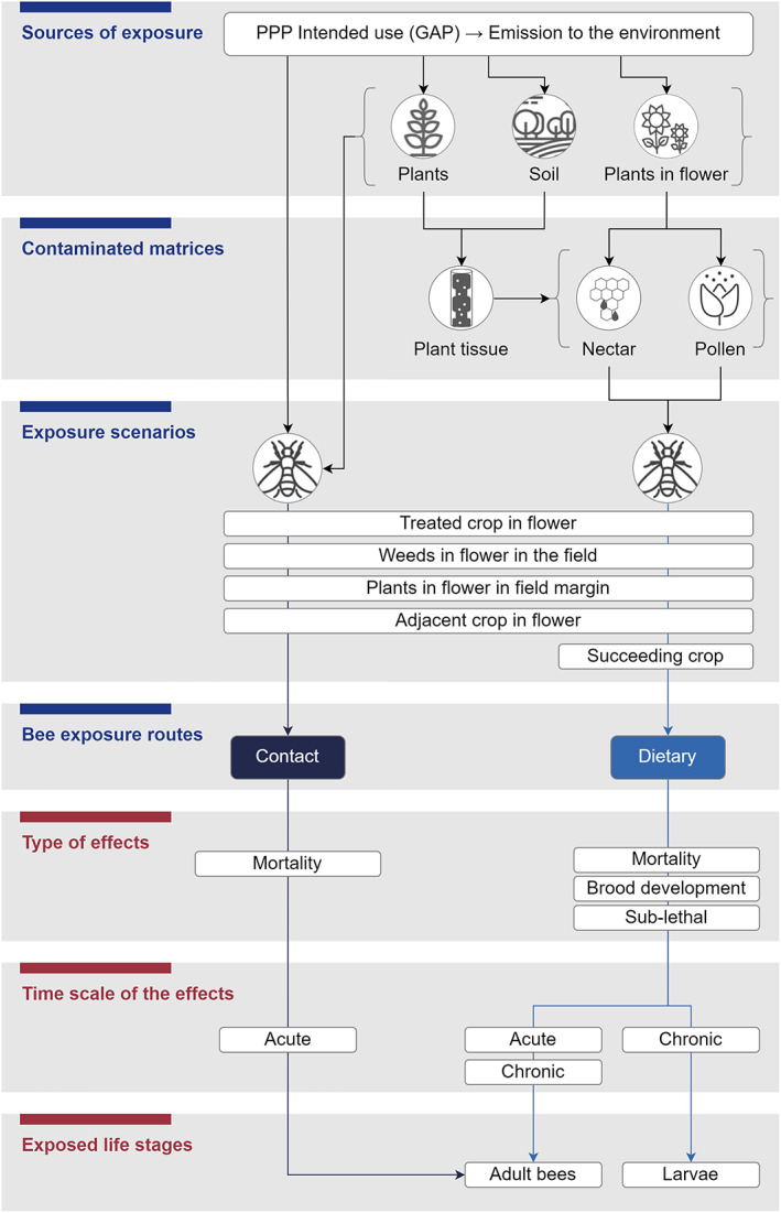
Bee exposure pathways evaluated in this guidance document and possible effects in time. It is noted that exposure via contaminated matrices other than pollen and nectar or exposure via inhalation are not included in the figure, since this was not specifically evaluated in this guidance
The methods of application of PPPs together with the crop‐growing systems included in the GAP determine the emission of a PPP in the environment and the way it can become a source of exposure for bees. Bees may come into direct contact with PPPs, as well as be exposed via contaminated matrices.
Environmental matrices may be contaminated directly (e.g. by spray liquid or dust deposits to the pollen/nectar) or via a series of processes: For example, (1) a PPP is sprayed onto the plant surface (e.g. leaves) → the PPP enters the plant and is distributed through the plant tissue → reaches the reproductive organ(s) → excreted into e.g. pollen and nectar; (2) a proportion of the PPP is sprayed onto the soil → PPP is taken up by the roots of the plant → distributes within the plant → reaches the reproductive organ(s) → diffused to e.g. pollen and nectar.
Bees may encounter PPPs or contaminated matrices either in areas treated with the PPP (in‐crop) or in areas which were not directly treated but have been unintentionally contaminated (off‐crop areas). In order to describe the agricultural areas where bees may be exposed to PPPs, various exposure scenarios have been defined:
Treated crop;
Weeds in the field unintentionally contaminated or intentionally treated;
Plants in the field margin unintentionally contaminated;
Adjacent crops: unintentionally contaminated;
Succeeding crops unintentionally contaminated through the soil.
The relevance and the level of the exposure in those scenarios vary pending on the GAP (see Chapter 4 and Chapter 5).
There are two main ways (i.e. bee exposure routes) through which a PPPs or their residues can reach bees (different life stages) in the above defined scenarios and potentially cause adverse effects:
By contact: occurs when bees enter in physical contact with the PPPs or with contaminated matrices, but does not involve ingestion;
By dietary: occurs when bees orally consume contaminated material and therefore, they ingest residues of PPPs with their diet.
Exposure to worker bees covers the exposure to various adult stages (e.g. drones, queens).
Insufficient information was available to consider the exposure through inhalation (see supplementary document). In some papers, it is reported as a minor route of exposure for most PPPs (Sanchez‐Bayo and Goka, 2014) and less relevant than contact and dietary (Crenna et al., 2020). Although not routinely addressed in this guidance, in some situations, a case‐by‐case basis consideration may be needed (see Section 4.2).
In this guidance, contact exposure is considered as the result of both overspray and contact of adult bees with contaminated surfaces shortly after the application of PPP. It is an acute exposure that may cause lethal effects. Contact exposure that can occur in situations such as, e.g. a bee walking repetitively on contaminated surfaces is considered unlikely and less relevant. In fact, it was demonstrated in the available data (Koch and Weisser, 1997) that the PPP mass on bees from contact exposure decreases very rapidly. Therefore, the guidance does not cover repeated and long‐term contact exposure, since it is not expected that the contact exposure of an individual increases after multiple applications. However, it is acknowledged that for most species of bumble bees and solitary bees nesting in the soil and cavities, repeated exposure by contact with contaminated soil/mud/leaves may be relevant, as already reported in the EFSA PPR Panel (2012). However, insufficient information is still currently available to address these exposures (Gradish et al., 2019; Sgolastra et al., 2019).
Dietary exposure is considered as ingestion of contaminated nectar and pollen by both adult bees and larvae that could cause lethal or sublethal effects on acute and chronic basis. Other contaminated matrices (e.g. honey dew, extrafloral nectaries, resin, wax, etc.) that could lead to oral residue intake (Requier and Leonhardt, 2020) are not explicitly covered in this guidance due to lack of sufficient data to propose a quantitative risk assessment approach. Some considerations on honey dew and extrafloral nectaries are given in Section 4.3.1.
The WG has evaluated the relevance of the exposure via consumption of contaminated water by considering the possibility of quantifying water consumption and the frequency and magnitude of water collection. However, data were not sufficient to achieve a reliable estimation of either aspect. In consideration of this, the WG has taken the decision not to include exposure from this contaminated matrix in the risk assessment. More details and data analysis concerning this decision are included in Annex E of the supplementary document.
The WG recommends that the areas above mentioned which are not covered in this guidance are addressed in a future revision of the guidance document and recognises the need to generate further research and data (see Chapter 15). Overall, addressing the knowledge gaps in relation to aforementioned bee exposure routes and to other matrices is pivotal for complementing future risk assessment of bees.
2. Scope of the guidance document
This document is intended to provide guidance to applicants and risk assessors for the risk assessment of bees in the context of the evaluation of PPPs and their active substances under Regulation (EC) No 1107/2009 for authorisation process at Member State level and the approval at EU level, respectively. In particular, this guidance covers risks that may occur when directly exposed to PPPs. Effects caused indirectly by the use of PPPs such as, e.g. removal of weeds in flower by herbicides, or direct (and indirect) effects on other insect pollinators are out of its scope.
The guidance document covers the risk assessment for chemical active substances, mainly applied as spray, seed treatment and granules, although the principles of the proposed risk assessment schemes are relevant for other methods of application. The guidance document does not cover the risk assessment for microorganism active substances for which specific considerations are needed and does not cover semiochemicals (including natural‐identical synthesised molecules) for which specific considerations are needed as mentioned in the guidance document SANTE/12815/20147.
Furthermore, the focus of this guidance is on the technical mixtures of active substance(s) and their co‐formulants undergoing an authorisation procedure with the Regulation (EC) No 1107/2009. It is acknowledged that bees can typically be exposed spatially and temporally to multiple residues (e.g. mix of insecticides, fungicides and herbicides) in the agricultural areas. However, the guidance does not address the risk assessment of combinations of more than one PPP of unknown composition or when PPPs are applied sequentially within one season (More et al., 2021).
3. Overview of the risk assessment
3.1. General principles
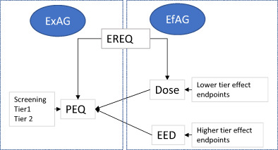
The implementation of the currently agreed SPGs in the risk assessment requires the combined evaluation of the exposure generated by the use of a PPP in the field (which can be predicted, simulated or measured) and of the ecotoxicological effects (which are assessed as part of the hazard characterisation based on an imposed exposure in the laboratory or higher tier effect experiments). To define in a structured and unambiguous manner, what exposure and which ecotoxicological effects should be used to implement the SPGs, the concepts of exposure assessment goal (ExAG) and effect assessment goal (EfAG) have been developed. The ExAGs relate to e.g. definition of the environmental exposure, type and duration (see supplementary document for more details) and EfAGs relate to e.g. definition of relevant model species, type of toxicity endpoints.
The definition of the ExAG allows to answer questions such as:
where, in which matrix and for what time frame the exposure should be estimated; or
what level of conservativeness the exposure estimate should aim for, i.e. what percentage of the exposure situations in the field should be covered in the risk assessment?
The definition of the EfAG allows to answer questions such as:
what should be the measured endpoints for the relevant species;
what extrapolation approaches should be used to cover other species, endpoints and untested exposure regimes; or
which percentile of a probabilistic effect assessment should be selected?
Bees will experience various levels of exposure to a PPP in agricultural areas following its use. This variability may be due to temporal differences (e.g. the same hive/nest may experience different exposure levels in spring vs. during summer) or due to spatial differences (e.g. different hives/nests placed at different locations in the area of use of the PPP). Therefore, the ExAG needs to define the percentile that represents the ‘realistic worst‐case’ exposure from the distribution of the various levels of the exposures. Since a 90th percentile is commonly used in ecotoxicology risk assessment e.g. for the EU FOCUS surface water scenarios, for this guidance document the 90th percentile, already used in EFSA (2013a,b), should be retained. However, while for the dietary exposure route, the (spatial) 90th percentile EREQ value could be estimated, no exact percentile could be determined for the contact exposure route, due to data limitations (for details, see Section 3.2 of the supplementary document).
3.2. Tiered approach
According to the ExAGs and EfAGs, both exposure estimation and effect assessment can be performed following a tiered approach, moving from relatively simple, conservative assessments to more realistic assessments. In fact, the concept of tiered approaches is to start with a simple assessment such as a screening, or Tier 1 and add reality and complexity by moving to Tier 2, or higher tier, if necessary to refine the risk i.e. when a high risk is not excluded at the lower tier. Since both the exposure and effect assessments are operationalised in the tiered approach, it is appropriate to define an exposure‐tier and an effect‐tier, separately.
The exposure and the effect (or hazard) tier assessments should address coherently the agreed SPGs in all the tiers and thus should be completely consistent with each other; for example, the effect assessment for honey bees focuses on hives located at the edge of treated fields, and thus, the exposure assessment should not include hives located far from pesticide‐treated agricultural areas.
Both the ecotoxicological endpoints and the exposure in the field can be defined through the concept of ecotoxicologically relevant exposure quantity (EREQ), which can be described as a type of quantity, that gives the best mechanistic link between exposure in the field and effects in an ecotoxicological experiment. Therefore, they should be expressed as the same type of exposure quantity (e.g. μg/bee per day) in order to enable a consistent linking between each effect and exposure assessment tier (see supplementary document for more details).
A summary of the key terms introduced in the risk assessment of this guidance document is reported in Table 2.
Table 2.
Definition of key terms used in this guidance
| Terminology | Explanation |
|---|---|
|
EREQ Ecotoxicologically Relevant Exposure Quantity |
Not a value, but a type of quantity, that gives the best mechanistic link between exposure and effects in an ecotoxicological experiment, and that is calculated/estimated both in the field (PEQ) and the ecotoxicological tests (dose/EED) |
|
PEQ Predicted Exposure Quantity |
A value; i.e. the quantification of an EREQ for a specific compound in the field/area of use. |
| Dose | A value: administered exposure in laboratory ecotoxicological tests |
|
EED Estimated Exposure Dose |
A value: estimated exposure in effect field studies |
| |
A fundamental aspect of the tiered approach is that every tier of the exposure assessment should address the same ExAG, every tier of the effect assessment should address the defined EfAG.
For both exposure and effect‐tier assessment, the routes of exposure for bees should be addressed by considering the different timescales of effect (acute and chronic) and the different life stages (adults and larvae).
To this purpose, four risk cases have been defined:
Acute‐contact risk;
Acute‐dietary risk;
Chronic‐dietary risk;
Larvae‐dietary risk.
An overview of the exposure‐Tiers and effect‐Tiers implemented in this guidance document is described in the following sections and also reported in Figure 2, below.
Figure 2.
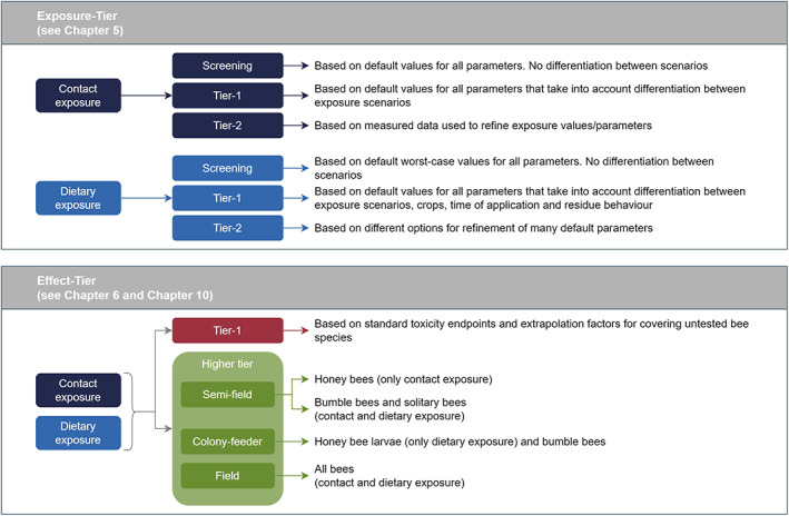
Tiered approach and explanations what each exposure or effect‐tier implies for the risk assessment of active substance. According to the principle of the tiered approach, each exposure‐tier can be linked to each effect‐tier
3.2.1. Exposure‐tier
In the exposure‐tiers, residue intake or residue deposition must be quantified by calculating the PEQ to address the dietary and contact routes of exposure of the bees following the use of a PPP in the field. The exposure estimation in the different tiers will provide PEQ for each of the above risk cases and it is indicated as PEQj, where the suffix j indicates the four risk cases.
Different models for the estimation of the PEQj are proposed in Chapter 5 of this guidance:
Contact exposure model;
Dietary exposure model through soil;
Dietary exposure model for application before the flowering period of the crop;
Dietary exposure model for applications during the flowering period of the crop.
Each of the above, calculates PEQj for the different exposure scenarios (see Figure 2).
In the lower tiers of the exposure assessment, the exposure is based on default parameters, while in higher tiers, the exposure of the colony (or population) may be based on measured parameters (e.g. PPP concentrations measured at the plant or brought into the hive/nest by bees, see Annex B – Recommendations for higher tier exposure studies).
3.2.2. Effect‐tier
The effect‐tier assessment is based either on laboratory studies with individual bees (adults or larvae) at the lower tier or semi‐field or field studies with colonies or populations (see Chapter 10) at the higher tier.
The laboratory studies give the dose–responses for the different timescales of the effect (acute and chronic) and different life stages (adult and larvae) and therefore address the four risk cases mentioned above in parallel with the estimation of PEQj. They are the basis for identifying the endpoints (see Chapter 6) for honey bees, bumble bees and solitary bees.
If there is evidence that the PPP under evaluation has a very specific mode of action (MoA) that affects a life stage or process that is not included in the standard data set (e.g. disruption of egg laying), specific additional data may be needed.
Higher tier studies, depending on the study type e.g. semi‐field, colony feeder and/or field tests (see Annex C – Recommendations for higher tier effect studies), provide a range of effect endpoints. In such studies, effects must be investigated at an exposure level in line with the ExAG, i.e. the 90th percentile worst‐case exposure for the compound under evaluation. Therefore, appropriate exposure regimes and levels, defined as Estimated Exposure Dose (EEDj), have to be ensured in the study and expressed in the same unit as the PEQj (see Chapter 10). This means that, in addition to the biological observations, it may be necessary to verify the exposure levels e.g. via measurement of residues in pollen and nectar, and use these measurements to estimate the EEDj in the specific study, which need to be compared with the related PEQj in order to assess if levels of exposure in higher tier studies were adequate and therefore if observed effects (or lack of effects) can be linked to the ExAG. The comparison should be carried out with PEQj based on independent measured residue trials (e.g. Tier 2), but if not available, the PEQj from lower tier exposure assessment will be used.
In this guidance, semi‐field, field and colony feeder studies are suggested for honey bees and bumble bees, while semi‐field and field studies are available for solitary bees (see Figure 2 and Chapter 10). They represent different levels of realism and complexity and provide different endpoints that can be compared with the SPG for honey bees or evaluated analytically for bumble bees and solitary bees, since the magnitude dimension of their SPGs is not defined.
The field tests represent the highest level of experimentally feasible effect assessments on bees foraging at local and larger scales (treated field, immediate off‐field areas and possibly landscape). In principle field tests can be supported by population‐level modelling of effects for different ecological and agricultural practice scenarios, but such models first would need to be developed, calibrated and evaluated for their use in regulatory bee risk assessment (see Section 10.6).
3.3. Risk assessment process
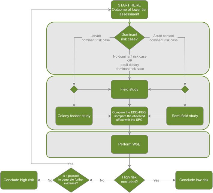
In this section, an overview of the scientific process for the risk assessment included in this guidance document is described by presenting the various steps, indicating when additional data should be generated. The overview for honey bees is given in the flowcharts in Figure 3 (for the lower tiers) and Figure 4 (for the higher tiers).
Figure 3.
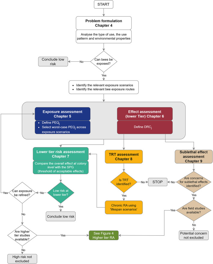
Overview of the lower tier risk assessment process for the active substance for honey bees (HB). Risk assessment of metabolites covered in Chapter 11. Risk assessment of mixture covered in Chapter 12. TRT = time reinforced toxicity (for honey bees). PEQj = predicted exposure quantity for the four risk cases (indicated by the suffix j) i.e. acute‐contact, acute‐dietary, chronic‐dietary, larvae‐dietary. Risk mitigation measures could be considered in the problem formulation to quantify the exposure reduction. Modelling could be considered as part of the higher tier assessment
Figure 4.
Overview of the higher tier risk assessment scheme for honey bees (for further details, see Chapter 10 and Annex C). EEDj = Estimated Exposure Dose for the four risk cases (indicated by the suffix j) i.e. acute‐contact, acute‐dietary, chronic‐dietary, larvae‐dietary
An important and primary component of the risk assessment process is the definition of a proper problem formulation that allows identification of cases where a risk assessment is not needed as well as selection of the more appropriate risk assessment methodology (see Chapters 4 and 10).
Based on the problem formulation, when exposure to bees cannot be excluded, exposure estimation and effect assessment should be performed in order to identify the worst‐case PEQj and the relevant effect endpoints for each of the four risk cases (see Chapters 5 and 6, respectively).
For the lower tier risk assessment, a combined approach which will integrate the different risk cases is proposed. The approach is described in Chapter 7; and allows calculation of the predicted individual level effect for each worst‐case PEQj, on the basis of the selected dose–response curve. The individual effects are extrapolated to the colony/population level effect based on a 1:1 relationship and then they are combined to predict the overall effect at colony/population level, which is directly compared to the SPG (i.e. a defined threshold of acceptable effects).
It is strongly recommended, based on the problem formulation, to start the risk assessment using the screening and Tier 1 exposure estimates. Depending on the outcome of this risk assessment, it is suggested to continue with the Tier 2 of the exposure. However, applicants could decide to address the risk identified in the Tier1 assessment directly by generating higher tier effect studies.
When a Tier 2 assessment is needed, applicants should generate appropriate data to replace the default values used in Tier 1.
When a low risk cannot be concluded based solely on the exposure refinement (i.e. exposure‐Tier 2), a higher effect‐tier assessment is required, and applicants should generate studies investigating the effects under realistic worst‐case use conditions for the concerned bee group.
As part of the effect‐tier assessment of the PPP, two additional aspects should in parallel be addressed at lower tier for honey bees: the potential for the compound under evaluation for showing increasing toxic effects due to long‐term exposure to low doses, and sublethal effects i.e.:
Time reinforced toxicity assessment (TRT) (see Chapter 8);
Potential concerns due to sublethal effects (see Chapter 9).
TRT assessment is determined via extrapolation from the standard 10‐day chronic honey bee toxicity study (OECD 245). It is important to note that when TRT is observed, it should be reflected by a proper selection of the honey bee chronic endpoint and by a proper risk assessment. In particular, both the toxicity endpoint and the exposure estimation (PEQj) should cover the whole lifespan of a honey bee, and therefore, two scenarios for risk assessment were considered for covering the active period of the bees (i.e. ‘summer bee scenario’), and an inactive winter period (i.e. ‘winter bee scenario’). Regarding sublethal effects, the WG has developed a preliminary assessment approach, in which the Tier 1 allows to identify potential concerns which could be addressed with further testing and/or go for a higher tier assessment with field studies, when those concerns cannot be excluded. However, a link between sublethal effects and the agreed SPG cannot currently be established (see Chapter 9).
As part of the risk assessment process, also the risk from metabolites should be addressed. A risk assessment scheme is proposed on this guidance which has to be followed together with the evaluation of the PPP (see Chapter 11).
In this guidance, a proposal is also provided for the risk assessment of mixture. This is not routinely included as part of the risk assessment processes of the active substance, but it may be mainly relevant within the authorisation of PPP at national level (see Chapter 12).
Risk mitigation measures (RMMs) can be integrated to an exposure assessment re‐estimation at any tier, except the screening level (See Chapter 13) and/or they can be proposed to reformulate the problem formulation. In both cases, in the context of the risk assessment, RMMs should be proposed by the applicant and mentioned in the good agricultural practices (GAP). When risk mitigation measures are integrated in the GAP, then the relevant exposure assessment should account for the suggested mitigation. In some cases, this will need the provision of exposure data while in other cases, default values are available (e.g. spray‐drift reduction) and can be used for the exposure assessment. It is considered essential that any suggested mitigation is demonstrated to reduce the risk sufficiently so that the specific protection goal is met (i.e. a risk assessment indicating a low risk).
Any higher Tier risk assessment can, in principle, be supported by colony or population‐level modelling. Such support could, e.g. consist of using a honey bee colony model to simulate the exposure as observed in an exposure field study with the aim of understanding the effect of, and whether it is possible to extrapolate to, other locations or environmental conditions. In addition, effectiveness of suggested risk mitigation measures (RMMs) for different ecological and agricultural practice scenarios could be assessed with the support of ecological population or colony models. In any case, any model first would need to be evaluated and tested for use in regulatory bee risk assessment following good modelling practices (EFSA PPR Panel, 2014). In addition, the use of ecological modelling as higher Tier refinement method in isolation is not considered as an option. More details on the possibilities for the use of ecological models are given in Chapter 10.
4. Problem formulation
Problem formulation is the first step of the risk assessment which allows applicants and risk assessors to identify the potential exposure pathways for a PPP and hazard and to formulate risk hypotheses and identify the proper risk assessment methodology. The problem formulation sets the boundaries for risk assessment for making it ‘fit for purpose’. For a risk to occur, it requires an exposure to a PPP which should result in a direct harm to the bees that exceeds a specified SPG. The use of PPPs may directly affect bees, or indirectly by impacting on their habitat and/or food availability. For example, a toxic effect on a bee would be considered a direct effect. Alternatively, the use of a herbicide may reduce the number of weeds in flower which in turn may reduce the available food in the bee's habitat, negatively impacting on individuals/colonies/populations of bees. The latter would be an example of indirect ecological effect. Although such ecological effects are relevant and should be addressed, this guidance document only considers direct toxicity‐mediated effects. The ecological effects can be addressed by ensuring that future EFSA guidance documents for PPP risk assessment sufficiently consider the supporting ecosystem service ‘food‐web support’ for bees (EFSA, 2023).
When evaluating a substance/compound, it is important to first determine, through a proper problem formulation, if and how, based on its intended use (i.e. GAP), it could reach the bees and estimate the level of the exposure (see Section 1.4). Therefore, the starting point is a careful consideration of the proposed uses of a PPP as indicated in the GAP table and an overall consideration of the physico‐chemical properties and the behaviour of the compound in environmental matrices (mainly molecular weight, water solubility, partition coefficient octanol/water, dissociation coefficient, vapour pressure, soil sorption, persistence in soil, formation and transformation products).
The first step (determining the occurrence of the exposure and identifying the most relevant exposure scenarios, considering the GAP) includes the analysis of:
the methods of application;
the crop(s) where the PPP is intended to be applied;
the crop phenology (i.e. BBCH).
If, based on this analysis, the exposure cannot excluded, it is necessary to identify the data needed for the effect assessment relative to the relevant route of exposure (i.e. contact/dietary), timescale of the effects and bee life stages, according to the data requirements (see Section 6).
The second step (defining the level of exposure) includes consideration of:
the application rate;
the number of applications;
and any particular conditions of PPP use.
Those aspects (also illustrated in Figure 5), overall, will allow applicants and risk assessors to understand the exposure pathways, to address the data requirements and to frame the risk assessment.
Figure 5.
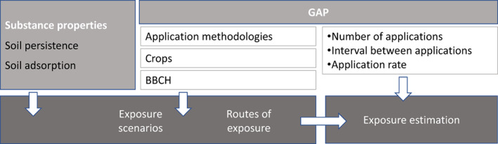
Elements of the GAP and physico‐chemical properties/behaviour of the compound in the environmental matrices determine the exposure scenarios, the route of the exposure and the bee exposure estimation to PPPs
4.1. Agricultural practices
A GAP table defines the way a PPP is proposed for use. It should include the following information (please note this list is not exhaustive):
Information on the PPP including the product type (e.g. a water dispersible granule), which active substance(s) is included and at what concentration;
The intended crops (or plants) and the growth stage of the crop (usually using the BBCH growth stage criteria). Time of year when applications will be made should be included in the GAP;
The Member States or regulatory zones where it is intended that the PPP will be used;
The intended application rate (normally in terms of amount of active substance per hectare, but the rate of the product may also be stated);
The number of applications and the application interval;
Limited information on the method of application (i.e. broadcast air assisted sprayer, seed treatment, etc.). The EPPO global database8 for PPP treatments is a useful source of application methodology;
Whether the PPP will be used indoors, in outdoor fields or in protected structures. According to EFSA (2014a,b), the type of protected structure should be defined (i.e. greenhouse or plastic tunnel);
Risk mitigation measures proposed by the applicant;
Other restrictions proposed by the applicant (e.g. applications are only allowed every 3 years);
Sometimes other information on how the PPP is intended for use may be stated (e.g. band application or spot application, the time between sowing of PPP treated seed and the start of flowering).
There are numerous other agronomic or growing practices which will influence the presence, and exposure, of bees in areas where the PPP will be used. If details of such practices are specified in the GAP, then it allows a risk assessment to account for them in the weight of evidence (see Section 10.6) and thus be more specific. Where information is lacking, a risk assessment should encompass (as far as practicable) all the conditions of where and how the PPP will be used. The following list includes the types of agronomic or growing practices which are expected to have an influence of the presence and/or exposure of bees (please note the list is not exhaustive):
Diversity of crops in the landscape;
Presence and type of between‐row vegetation;
Crop development stage at time of harvest;
Time between the application and the start of the flowering for spray applications;
For high‐growing crops (e.g. orchards, hops, vineyards) with spray applications, the effective dose rate of application expressed also as treated leaf wall area (tLWA).
4.2. Type of uses and application methods
During the problem formulation, it should be checked for each use in the GAP, whether the a.s./PPP under assessment is intended to be applied in open field or closed spaces.
The EFSA guidance EFSA (2014a,b) and EPPO Global Database 8 use the following categories:
Indoors and/or in permanent greenhouses (closed spaces);
Semi‐open structures (low mini tunnels, plastic shelters, net shelter/shade house and walk‐in tunnels);
Outdoor uses (open field).
For indoor uses and/or in permanent greenhouses, no exposure to bees living in the surrounding areas is expected; therefore, a risk assessment is normally not necessary. However, it is noted that for applications made to seedlings, seeds or tubers which are subsequently transported to the field, exposure to bees may occur. In this case, a risk assessment is needed unless it is clearly stated in the GAP that transportation to the field will not happen. Equally for substances that are (semi‐)volatile, exposure may occur following deposition of the substance in the proximity of the closed space. In these cases, a risk assessment may be required (See Table 3, note 8).
Table 3.
Overview of the possible type of uses and methods of PPP application in relation to the contact and dietary routes of exposure in the exposure scenarios
| Contact | Dietary | |||||||
|---|---|---|---|---|---|---|---|---|
| Treated crop | Weeds* (treated field) | Field margin | Treated crop | Weeds (treated field) | Field margin | Adjacent crop | Succeeding crop/Permanent crop | |
| Seed treatment (coating) | N | N | Y | Y | N** | Y | Y | Y |
| Granular application | Y | Y | Y | Y | Y | Y | Y | Y |
| Conventional spray applications | Y | Y | Y | Y | Y | Y | Y | Y |
| Other spraying methods (i.e. aerial spray, in‐furrow, knapsack, stem application, etc…) (See note 1) | Y | Y | Y | Y | Y | Y | Y | Y |
|
Brushing, Wiping Application of a liquid product or powder with a brush |
N | N | N | Y | N | N | N | Y |
|
Injecting Application of a liquid product or solution by injecting it directly into the treated object |
N | N | N | Y | N | N | N | Y |
|
Dipping Application by immersing the treated object or part of it in a liquid product or solution (See note 2) |
N | N | N | Y | Y | N | N | Y |
|
Drenching Application of a liquid product or solution by pouring over the treated object (See note 3) |
N | N | N | Y | Y | Y | Y | Y |
|
Dripping Application of a liquid product or solution via multiple drops on substrate or soil |
N | N | N | Y | Y | N | N | Y |
|
Placing Application by positioning a product within target range (See note 4) |
N | N | N | Y | Y | N | N | Y |
|
Circulating water application Application of a product in the nutrient solution that it is circulated in a closed system to irrigate plants growing in substrates Presumed protected use (See note 8) |
N | N | N | N | N | N | N | N |
|
Dusting Application of a product by blowing tiny solid particles (dustable powder) towards the treated object |
Y | Y | Y | Y | Y | Y | Y | Y |
|
Fogging Application of a product by producing an atmosphere full of tiny droplets (particle size 0.05–50 μm) |
Y | Y | Y | Y | Y | Y | Y | Y |
|
Fumigating Application of a product that completely fills a confined space in a gaseous form (See note 5) |
Y | Y | Y | Y | Y | Y | Y | Y |
|
Impregnating Application of a liquid product or solution for absorption by a solid object (See note 6) |
Y | N | N | N | N | N | N | N |
| Soil incorporation (as soil fumigants) (See note 7) | N | N | N | N | N | N | N | N |
| Permanent greenhouse (See note 8) | N | N | N | N | N | N | N | N |
The relevance of this scenario also depends on the BBCH (see Section 4.3.2).
The scenario might be relevant if residues are absorbed and translocated from the soil through the plant tissues, and later translocate to nectar and pollen of the weeds in flower.
For semi‐open structures and outdoor uses, exposure cannot be excluded, and thus, a subsequent consideration of the application methodologies is needed to understand how and where the bees can be exposed. Semi‐open structures are assessed as outdoor uses.
The most frequently used application methods that may lead to bee exposure are spraying of a liquid (emulsions, suspensions or solutions), seed treatments and distribution of granules. The present guidance covers mainly these methods of applications, for which exposure estimation approaches are available and consolidated. However, bee exposure to PPP applied with other methods of application cannot be excluded. When a PPP is intended to be applied using an application method which is not covered by this guidance, including modern technologies, it is considered that the applicant has the responsibility to provide a proper characterisation of the exposure in line with the principles of this guidance (see Chapter 5).
An overview of the most common methods of application is reported in Table 3 together with a consideration of the relevance of exposure scenarios (see Section 4.3) in relation to the routes of exposure (see Section 1.4). The list was compiled based on the definition of EPPO nomenclature9 and/or other existing uses registered in EU, although it may not be exhaustive.
4.2.1. Notes to the possible type of uses and methods of PPP application
In this section, additional remarks mentioned as notes in Table 3 are reported.
As general remark, it is highlighted that for the uses reported in the Table 3 particular methods of application such as band application, spot application, treatment between the row, etc., have also been taken into account.
For uses in semi‐open structures, exposure cannot be excluded. Therefore, they must be considered as field uses.
NOTE 1 on other spraying methods.
The off‐crop (i.e. field margin, adjacent crop) exposure of some of these methods of spraying may not be covered by the standard drift values used in the GD (e.g. for applications via helicopters, drones, etc.). Also, for other methods (e.g. stem application), flowers are not directly sprayed. For in‐furrow applications, the product is applied together with the seed along the line drawn by the plough. Consequently, the exposure pathways differ for each of these methods and should be properly characterised.
NOTE 2 on dipping.
Bulbs, plants roots or entire seedlings are dipped in the product (or a solution of the product) before planting in the field. The seedlings have no flower at the time of application nor do they have them shortly thereafter. A distinction should be made if soil surrounding the roots is also dipped into the product or just the bulb/roots. In the former case, dietary exposure via the weeds may also be possible. Sometimes, plant trays are dipped in the product.
NOTE 3 on drenching.
Drenching can be via a boom sprayer without the use of nozzles. In this case, there is no atomisation of the liquid and the majority of the liquid reaches the soil. No drift is assumed from this kind of application, but exposure might be possible via soil contamination in the off‐crop e.g. via run‐off. The outcome of any evaluation with this application technique is pending on the height and the accuracy of the device used for the application.
NOTE 4 on placing.
A solid object (rodlets, sticks, etc…) placed directly in the soil, besides the plants. Exposure might be possible via soil contamination.
NOTE 5 on fumigating.
Despite being applied in a confined space, re‐entry of workers may require opening the windows for ventilation. Off‐crop exposure may then be relevant in some cases.
NOTE 6 on impregnating.
The applications of a liquid product for absorption by a solid object e.g. in nets impregnated with an insecticide or in traps in combination with an attractant are designed to kill pests (if the attractant serves as a food source, the oral exposure should be assessed in addition to the contact exposure). The potential of exposure should be properly characterised depending on the design (accessibility and/or attractivity).
NOTE 7 on soil incorporation (as soil fumigants).
Soil fumigants may be injected (as liquids forming gas) into the soil and move through the soil mainly via diffusion in the gas phase. Exposure of bees in the air above and around the field of application is likely. Exposure to the off‐crop via redeposition is likely if the treated soil is not properly sealed after application. This may lead to contamination of flowering plants growing outside the treated area (directly or via soil) and exposure of bees (contact and oral). A very specific exposure pathway is exposure via inhalation, which may be relevant for highly volatile substances such as soil fumigants under certain circumstances. Inhalation toxicity studies can then be an option for the risk assessment.
NOTE 8 on permanent greenhouse.
In contrast to the entry in Table 4, exposure cannot be excluded for items that are moved outside and for (semi‐)volatile substances. If plants, seeds or tubers are moved outside after treatment, exposure (contact and dietary) may result from these treated items. For these uses, exposure to bees cannot be excluded and the risk assessment should be performed by considering the items moved outside for the treated crop scenario and succeeding crop scenario.
Table 4.
Relevance of contact and dietary exposure for pollen/nectar attractive crops
| Attractive crop | |||
|---|---|---|---|
| Before flowering | Flowering | Post‐flowering or harvested before flowering | |
| Contact exposure | No | Yes | No |
| Dietary exposure | Yes | Yes | No |
If the active substance is (semi‐)volatile, deposition from the air to the area in the vicinity of the greenhouse or closed building may occur following venting. This may lead to contamination of flowering crops and plants growing outside the greenhouse/building (directly or via soil) and exposure of bees (contact and dietary). When deposition rate is calculated in the fate and behaviour section, this should be taken for the bee risk assessment.
4.3. Exposure scenarios
As explained in Section 1.4, several exposure scenarios have been defined, since bees may be exposed in the treated areas (i.e. treated crop and weeds in flower scenarios) and/or in the surrounding areas (i.e. field margin and adjacent crop scenarios). Furthermore, in some situations, bees may be exposed to residues in the pollen and nectar that are taken‐up by the crops growing after the one under evaluation (i.e. succeeding crop scenario).
In those scenarios, bees may be exposed by contact and/or via the diet (in some situations by inhalation).
Depending on the GAP, during the problem formulation, the occurrence of (acute and/or dietary) exposure from some scenarios can be excluded a priori (see Table 3). In these cases, the exposure estimation is required only for the remaining relevant scenarios and/or routes of exposure (e.g. when the PPP is applied as brushing or wiping, contact exposure is not anticipated in any scenarios while dietary exposure may be expected in treated crop, depending on the crop and BBCH, or succeeding crop depending on the physico‐chemical properties of the PPP).
It is noted that exploring the possibility of applying risk mitigation measures at Tier 1 or Tier 2 before going to the higher tier studies could be an option to reformulate the problem formulation, when exposure reduction is demonstrated (see Chapter 13).
4.3.1. Treated crop
The exposure of bees to PPPs in the treated areas requires that bees visit and interact with crops; therefore, it is necessary to ascertain if crops in the GAP are attractive to bees. As pollen and nectar are the main sources of nutrition for bees, the WG defined a crop as being attractive based on the presence and availability of pollen and nectar. The WG decided that any crop that meets one of the following criteria is considered attractive to bees:
The crop produces nectar which is accessible to bees;
The crop produces nectar and pollen which is accessible to bees.
There is a third group of crops which produce pollen but no nectar. Within this third group, there are crops which are frequently visited by bees (e.g. poppy seed), while others are not. To distinguish between these crops, EFSA has performed an Expert Knowledge Elicitation (EKE) according to EFSA (2014a,b). The details of the EKE are reported in Section 4.3.1 of the supplementary document and its Annex F. Based on the results of the EKE, the WG revised the list of attractive crops for bees and has made a new list that is available in the Appendix A – Crop attractiveness.
When a crop is attractive to bees for pollen and/or nectar, bees can be exposed in the treated crop scenario both by contact and via the diet. To further assess the relevance of the treated crop scenario, it is necessary to consider:
Table 5.
Overall conclusion on the relevance of the weed scenario for the contact risk assessment for different crops and their respective BBCH stages at the time of application
| Crop | BBCH stage (at the time of application) | |||||
|---|---|---|---|---|---|---|
| 0–9 | 10–19 | 20–29 | 30–39 | 40–49 | 50–99 | |
| Sunflower | No | No | – | Yes 2 | Yes 2 | Yes 2 |
| Maize | No | No | – | Yes 2 | Yes 2 | Yes 2 |
| Winter oilseed rape | No | No | Yes 2 | Yes | Yes | Yes |
| Winter cereals | No | No | No | Yes | Yes | Yes |
| Sugar beet 3 | No | No | – | No | – | No |
| Potatoes | No | No | No | No | No | No |
| Peas | No | No | – | No | Yes 2 | Yes 2 |
| Bean | No | No | No | No | Yes 2 | Yes 2 |
| Other arable crops 1 | No | No | Yes 2 | Yes 2 | Yes 2 | Yes 2 |
| Permanent crops | Yes | |||||
Notes: ‘No’ indicates that the scenario is not relevant, and that a risk assessment is not needed, ‘Yes’ indicates that the scenario is relevant, and that a risk assessment must be performed.
Including spring cereals and spring oilseed rape, and all other annual and biannual crops such as fruiting vegetables, leafy crops, bulbs, etc.
The data available are not sufficient for a conclusion, or no data is available at all. Therefore, the weeds scenario is considered relevant for the time being. This conclusion could potentially be revised when further data become available.
Unless cultivated for seed production, sugar beet is harvested at BBCH 49; −: BBCH stage does not exist for this crop according to the BBCH Monograph (Meyer, 2001).
When a crop is considered not attractive, the exposure is assumed to be zero, and therefore, the treated crop scenario is not relevant.
It is noted that for some crops, extrafloral nectaries may occur and consequently exposure via nectar may be relevant outside the flowering period. Since no data are available to estimate this exposure, when relevant, it should be considered an uncertainty in the risk assessment that could be addressed at Member State level by assuming that the application occurs when nectar is present irrespective of the BBCH indicated in the GAP.
The WG also acknowledged that in some situations when the crop is not attractive for nectar and pollen (e.g. cereals), honey dew could be a relevant source of exposure. Some available information of crops in which honey dew can be present is included in the Appendix A of the supplementary document. This information is not exhaustive. It is based on pest pressure and control in The Netherlands and it is unknown if it can be extrapolated to other countries. However, it may be useful at Member State level for a further consideration of this aspect, which is not covered in the current guidance document.
If the GAP table refers to a crop which is absent from Appendix A – Crop attractiveness, the applicant should propose a surrogate crop with similar characteristics (morphology, phenology, etc.). The applicant should make it very clear that a surrogate has been used; they should also duly justify the choice of surrogate crop and how the selection was made. The selected surrogate crop will be considered by risk assessors. It is recommended that member state authorities be consulted regarding such a proposed surrogate early in the application process, whenever possible.
4.3.2. Weeds in the treated field
When the ‘treated crop’ scenario is not considered relevant for the bee exposure, bees may still be exposed in the treated areas while foraging on the weeds in flower present in those areas. The relevance of weeds in flower in the treated field as an exposure source for bees was assessed based on the results from a re‐analysis of the data set from Last et al. (2019), in combination with the outcome of a consultation of efficacy experts. The full details on this analysis (i.e. data set used, steps in the re‐analysis, interpretation of the results, etc.) are reported in Section 4.3.2 of the supplementary document.
Based on the available data and analysis, the WG concluded that for both the contact and dietary exposure, in some situations, this scenario can be excluded a priori. When this is the case, there is no need to carry on with the exposure estimation. An overview of those cases where the weeds in flower scenario is or is not relevant for the contact route of exposure is provided in Table 5, and for the dietary route of exposure in Table 6.
Table 6.
Overall conclusion on the relevance of the weed scenario for the dietary risk assessment for different crops and their respective BBCH stages at the time of application
| Crop | BBCH stage (at the time of application) | |||||
|---|---|---|---|---|---|---|
| 0–9 | 10–19 | 20–29 | 30–39 | 40–49 | 50–99 | |
| Sunflower | No | No | – | Yes 3 | Yes 3 | Yes 3 |
| Maize | Yes 2 | Yes 2 | – | Yes 3 | Yes 3 | Yes 3 |
| Winter oilseed rape | Yes 2 | Yes 2 | Yes 2 | Yes 2 | Yes 2 | Yes 2 |
| Winter cereals | No | No | Yes 2 | Yes 2 | Yes 2 | Yes 2 |
| Sugar beet 4 | No | No | – | No | – | No |
| Potatoes | No | No | No | No | No | No |
| Peas | No | No | – | Yes 2 | Yes 3 | Yes 3 |
| Bean | No | No | Yes 2 | Yes 2 | Yes 3 | Yes 3 |
| Other arable crops 1 | Yes 3 | Yes 3 | Yes 3 | Yes 3 | Yes 3 | Yes 3 |
| Permanent crops | Yes | |||||
Notes: ‘No’ indicates that the scenario is not relevant, and that a risk assessment is not needed, ‘Yes’ indicates that the scenario is relevant, and that a risk assessment must be performed.
Including spring cereals and spring oilseed rape, and all other annual and biannual crops such as fruiting vegetables, leafy crops, bulbs, etc.
Relevance of the scenario could not be excluded based on the analysis currently performed (i.e. considering weeds at BBCH ≥ 30 – see Section 3.3 in Annex D to the supplementary document). This conclusion can be revised if further data on the presence of weeds covering also later crop BBCH stages become available.
No data are available. Therefore, the weeds scenario is considered relevant for the time being. This conclusion could potentially be revised when further data become available.
Unless cultivated for seed production, sugar beet is harvested at BBCH 49; −: BBCH stage does not exist for this crop according to the BBCH Monograph (Meyer, 2001).
If this exposure is relevant, depending on the GAP, an exposure estimation for this scenario is required in order to understand whether it may drive the overall exposure for bees.
The WG acknowledged that there are limitations and uncertainties related to the data set and analysis performed. Several conservative assumptions had to be made in order to allow for a conclusion based on the quantitative data available. If additional data become available to support more realistic assumptions, the analysis can be updated, and the conclusions could potentially be revised. In addition, further data could be submitted to address those situations for which data are currently lacking, and for which the weeds in flower scenario are assumed to be relevant for the time being. The WG developed recommendations for further addressing the current knowledge gaps (see Annex D of the supplementary document). Although detailed guidance could not be provided for generating fit‐for‐purpose monitoring studies, some general indications for such studies were provided. The exposure estimation for this scenario is described in Chapter 5.
4.3.3. Field margin and adjacent crop
Areas surrounding the treated crop can be defined as field margin (wild vegetation) and adjacent crops (agricultural crops grown by a farmer in the neighbouring field). In these areas, deposition from PPP applications may occur as consequence of spray drift (spray applications) or dust drift (after the sowing of treated seeds or application of granules). Depending on the GAP (see Table 3), the field margin (that represents a relevant area of interest for pollinator habitats) as well as the adjacent crops have to be considered as a relevant exposure scenario for both the contact and the dietary route of exposure. For these scenarios, it is assumed that plants/crops are in flower when the drift/dust event occurs.
Taking into consideration biological, ecological and meteorological aspects, three set‐ups were recommended by the WG. These are the following (see also in Figure 6 and Table 7 below):
Field margin A: Two metres widths and located immediately next to one of the sides of a rectangular treated field. It is assumed that the field margin is always downwind. This set‐up is to be used for the contact assessment for all the bees and for the dietary assessment for bumble bees and solitary bees;
Field margin B: Two metres widths and located immediately next to all the four sides of a rectangular treated field. The consequence of this physical set‐up is that – irrespective of the wind direction – one‐third of the field margin areas are contaminated due to spray drift or dust drift, while two‐thirds are located upwind thus remains uncontaminated. This set‐up is to be used only for the dietary assessment for honey bees;
Adjacent crop: it has 50 m widths and is next to a rectangular treated field. It is assumed that the adjacent crop is always downwind. This set‐up is to be used only for the dietary assessment for honey bees.
Figure 6.
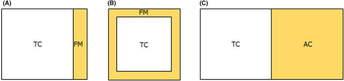
(A) Field margin A scenario for contact route of exposure for all bee groups and for the dietary exposure for bumble bees and solitary bees; (B) – field margin B scenario for the dietary exposure for the honey bees; (C) – adjacent crop scenario for the dietary exposure for honey bees (TC = treated crop; FM = field margin; AC = adjacent crop)
Table 7.
Summary of the relevance of the off‐field scenarios
| Scenario | Contact exposure | Dietary exposure |
|---|---|---|
| Field margin A | Relevant for all bee groups | Relevant only for bumble bees and solitary bees |
| Field margin B | Not relevant | Relevant only for honey bees |
| Adjacent crop | Covered by field margin A, therefore not used | Relevant only for honey bees, (covered by field margin A for the other bees) |
These considerations are reflected by the parameterisation of the exposure assessment that is described in Chapter 5.
It is noted that, as in EFSA (2013), no adjacent crop scenario for the contact exposure for honey bees is set, as this scenario is covered by the field margin scenario. Further background and explanation of the three set‐ups is included in Section 4.3.3 of the supplementary document.
4.3.4. Succeeding crop
In the succeeding crop scenario bees are exposed to pollen and nectar contaminated with residues of the substance (active ingredient and/or metabolites) that are already present in the soil following the treatment of the preceding crop. Residues that persist in soil are taken up by the roots of the succeeding annual crops or the permanent crops next year and then translocated via the vascular system and the tissues of plants to the nectar and pollen. This may also happen for the double crops: annual crops that are grown twice in a growing season on the same field (e.g. beans). As in EFSA (2013), it is considered that if the succeeding crops are not defined, it is assumed that the crops are attractive for both pollen and nectar.
The relevance of the succeeding crop scenario was re‐examined based on the available field studies where the residues levels of a substance were measured in pollen and/or nectar collected from a crop grown as follow‐on crop (see Section 4.3.4 of the supplementary document). In addition, a screening level was established in order to identify those substances that, for a specific GAP, would lead to an exposure level that will not cause adverse effects on bees for the succeeding crop scenario. Based on the available data and analysis, the WG concluded that for the dietary route of exposure, the succeeding crop scenario cannot be excluded a priori but its relevance should be always considered during the problem formulation. However, for the annual double crops and for the permanent crops the following year, the WG concluded that in some situations, this scenario can be excluded based on specific combinations of soil persistence (soil DegT50) and soil adsorption (Koc) properties of a substance with toxicity endpoints ≥ 0.1 μg/bee and at a given application rate (Tables 8 and 9). It should be noted that a necessary condition for the applicability of the screening level is that all the toxicity endpoints (i.e. all the acute LD50 values, the LDD50 and the larval ED50) must be ≥ 0.1 μg/bee, ≥ 0.1 μg/bee/day and ≥ 0.1 μg/larva/developmental period. When this is the case, then there is no need to further assess the succeeding crop scenario. The details on the screening level for the succeeding crop scenario are reported in Annex I of the supplementary document.
Table 8.
Screening level for the relevance of the succeeding crop exposure scenario based on different combinations of soil persistence (soil DegT50) and adsorption properties (Koc) of a substance and application rates (expressed as total annual application) to permanent crops. The screening level is applicable only when all the toxicity endpoints (i.e. all the acute LD50 values, the LDD50 and the larval ED50) are ≥ 0.1 μg/bee. When the properties of a substance meet one of the combinations, an exposure assessment of the succeeding crop scenario is not needed
| Application rate ≤ 100 g/ha | Application rate ≤ 500 g/ha | Application rate ≤ 1 kg/ha | Application rate ≤ 5 kg/ha | Application rate ≤ 10 kg/ha |
|---|---|---|---|---|
|
Soil DT50 ≤ 3 days Koc ≥ 100 mL/g |
Soil DT50 ≤ 3 days Koc ≥ 100 mL/g |
Soil DT50 ≤ 3 days Koc ≥ 100 mL/g |
Soil DT50 ≤ 3 days Koc ≥ 100 mL/g |
Soil DT50 ≤ 3 days Koc ≥ 100 mL/g |
|
Soil DT50 ≤ 10 days Koc ≥ 500 mL/g |
Soil DT50 ≤ 5 days Koc ≥ 500 mL/g |
Soil DT50 ≤ 5 days Koc ≥ 500 mL/g |
||
|
Soil DT50 ≤ 30 days Koc ≥ 2,000 mL/g |
Soil DT50 ≤ 10 days Koc ≥ 2,000 mL/g |
Soil DT50 ≤ 10 days Koc ≥ 5,000 mL/g |
||
|
Soil DT50 ≤ 60 days Koc ≥ 5,000 mL/g |
Table 9.
Screening level for the relevance of the succeeding crop exposure scenario based on different combinations of soil persistence (soil DegT50) and adsorption properties (Koc) of a substance and application rates (expressed as total annual application) to annual ‘double’ crops. The screening level is applicable only when all the toxicity endpoints (i.e. all the acute LD50 values, the LDD50 and the larval ED50) are ≥ 0.1 μg/bee. When the properties of a substance meet one of the combinations, an exposure assessment of the succeeding crop scenario is not needed
| Application rate ≤ 100 g/ha | Application rate ≤ 500 g/ha | Application rate ≤ 1 kg/ha | Application rate ≤ 5 kg/ha | Application rate ≤ 10 kg/ha |
|---|---|---|---|---|
|
Soil DT50 ≤ 3 days Koc ≥ 100 mL/g |
Soil DT50 ≤ 3 days Koc ≥ 100 mL/g |
Soil DT50 ≤ 3 days Koc ≥ 500 mL/g |
Soil DT50 ≤ 2 days Koc ≥ 100 mL/g |
Soil DT50 ≤ 2 days Koc ≥ 100 mL/g |
|
Soil DT50 ≤ 5 days Koc ≥ 500 mL/g |
Soil DT50 ≤ 5 days Koc ≥ 2,000 mL/g |
Soil DT50 ≤ 5 days Koc ≥ 5,000 mL/g |
Soil DT50 ≤ 3 days Koc ≥ 2,000 mL/g |
Soil DT50 ≤ 3 days Koc ≥ 5,000 mL/g |
|
Soil DT50 ≤ 10 days Koc ≥ 2,000 mL/g |
||||
|
Soil DT50 ≤ 30 days Koc ≥ 5,000 mL/g |
Chapter 5 provides guidance for the exposure assessment for the three types of succeeding crop scenarios.
4.3.5. Summary of the elements included in the problem formulation
In Table 10, below, an overview of the various aspects to be considered when performing the problem formulation to frame the risk assessment is presented.
Table 10.
Overview of the elements to be considered for the problem formulation to frame the risk assessment
| GAP | ||||
|---|---|---|---|---|
|
Crop Method of application Crop BBCH |
Method of application Crop BBCH |
Application rate Number of application (multiple application and time between application) Remarks |
||
| Identify the relevant scenario |
Identify the route of exposure Select the relevant exposure model |
Calculate PEQj | Select realistic worst‐case PEQ for each risk case | |
|
Treated crop ‐ > check attractiveness ‐ > check crop BBCH ‐ > check method of application |
Dietary |
Through soil Before flowering During flowering |
Dietary acute Dietary chronic Dietary Larva |
PEQdi,ac PEQdi,ch PEQdi,lv PEQcn |
|
Contact |
Contact model | Contact acute | ||
|
Weeds ‐ > check crop BBCH ‐ > check method of application |
Dietary |
Through soil During flowering |
Dietary acute Dietary chronic Dietary Larva |
|
|
Contact |
Contact model | Contact acute | ||
|
Field margin/Adjacent crop ‐ > check method of application |
Dietary | During flowering |
Dietary acute Dietary chronic Dietary Larva |
|
| Contact | Contact model | Contact acute | ||
|
Succeeding crop ‐ > check substance properties (soil persistence/adsorption) and application rate ‐ > check crop type |
Dietary | Through soil |
Dietary acute Dietary chronic Dietary Larva |
|
In relation to the dietary exposure via consumption of contaminated pollen and nectar, it has to be noted that the proportional contribution of the various exposure scenarios to the daily food intake by bees is unknown. Therefore, the WG has retained the assumption of EFSA (2013), that each scenario contributes to 100% of the contaminated food consumed by bees, as worst case. In theory, this might lead to stacking of selected exposure percentiles and thus extreme exposure probabilities. However, usually one of the exposure routes will strongly dominate the exposure, and thus, stacking of probabilities is unlikely to be an issue.
It is noted that among the most relevant scenarios, only those scenarios that will strongly dominate the exposure on the basis of the exposure estimation will be used for risk assessment, since the ‘dominant scenario’ is considered to cover all the others. This means that worst‐case PEQj will be selected across scenarios for risk assessment (see Chapter 4). It is important to note that the ‘worst‐case’ PEQj should be identified at each tier of the risk assessment. For example, if for a substance/compound and its intended use under evaluation at Tier 1, the ‘e.g. treated crop, or weed scenario’ is identified as giving the worst‐case PEQj (‘dominant scenario’) and the Tier 1 fails, at the Tier 2, all the scenarios should be reconsidered to redetermine the ‘dominant scenario’. This will ensure that by including the refinement options, the relevant ‘dominant scenario’ is always identified and the other scenarios are covered. Equally, when risk mitigation measures are applied at Tier 1 or Tier 2 (e.g. only apply outside the flowering period of the crop), the ‘dominant scenario’ should be redetermined.
5. Exposure assessment
This chapter contains (1) the mathematical models to be used for the exposure estimations for the different exposure routes covered by the risk assessments; (2) the parameters for the tier 1 exposure assessments; and (3) the refinement options. In addition, at the end of the chapter (Section 5.6), a screening exposure assessment is described. As summarised in Table 11, a single mathematical model may be applicable for several exposure scenarios.
Table 11.
Relevance of the dietary models for the different exposure scenarios
| PPP application | Exposure scenario | ||||
|---|---|---|---|---|---|
| Treated crop | Weeds in the field | Field margin | Adjacent crop | Succeeding crop | |
| BBCH < 10, ‘bare soil’ situation | Through‐soil contamination | Through‐soil contamination | During‐flowering contamination | During‐flowering contamination | Through‐soil contamination |
| BBCH < 10, presence of emerged weeds not excluded | Through‐soil contamination | During‐flowering contamination | |||
| BBCH 10–59 | Pre‐flowering contamination | ||||
| BBCH 60–69 | During‐flowering contamination | ||||
| BBCH ≥ 70 | Not relevant | ||||
5.1. The exposure assessment models
The exposure assessment models (i.e. the mathematical expressions of the exposure estimation) described in this section are to be used to predict the exposure quantity (PEQ) of an individual bee for the two main routes of exposure (i.e. contact and via diet) arising from the application of a PPP. These predictions are to be used in both the lower and the higher tier risk assessments (see Chapters 7 and 10). The model to be used for the contact route of exposure is included in Section 5.1.1 and the models to be used for the dietary exposure route are in Section 5.1.2.
Other routes of exposure, such as inhalation, could be relevant (see Chapter 4). However, exposure models and default parameters for such exposure routes are not available. Therefore, in such situations, applicants should generate fit for purpose data for characterising the exposure.
5.1.1. Contact model
Contact exposure is a form of acute exposure that requires physical contact between the PPP and the surface of the bee (see Section 1.4). This may happen during (e.g. direct overspray), or shortly after (the bee interacts with a surface where PPP have been deposited) the PPP application; therefore, this route of exposure is relevant for foraging honey bees, foraging worker bumble bees and adult solitary bees.
The model for this route of exposure is described by the following equation:
| (1) |
where:
PEQco: Predicted Exposure Quantity for contact exposure – μg/bee.
In other parts of the guidance document, PEQ is indexed with a ‘j’ since PEQ is used for different risk cases (‘j’ refers in general to the risk cases), here the acute contact risk case is indicated by the suffix ‘co’.
AR: application rate – g/ha.
EFco: exposure factor for contact exposure (−).
BSF: body surface factor – dm2/bee.
The detailed descriptions of the parameters are included in Section 5.2.
The contact model as described above is applicable for all types of application methods covered in this guidance document, for all relevant scenarios and for all bee groups.
5.1.2. Dietary models
The dietary exposure assumes that adult bees or the bee larvae come to contact with the PPP via consumption of contaminated food (pollen and or nectar). As indicated in Section 1.4, acute and chronic dietary exposure is considered in this guidance document for adult bees and chronic exposure for larvae. It must be noted that pending on the toxicity profile of the PPP (i.e. when a fast expression of effects is observed in the chronic laboratory test for adults), the estimation for the acute exposure should be used in the risk assessment even for the chronic adult risk case (for further explanation, see Section 6.6).
Three models considering numerous parameters to estimate the quantity of the PPP residue per bee were created. The first model predicts residue intake when the contamination of pollen and nectar originates from the residue uptake process from soil (see Section 5.1.2.1). The second is for situations when the contamination of pollen and nectar dominantly originates from contamination of the above‐soil parts of the crop before its flowering stage (see Section 5.1.2.2). The third model predicts the residue intake for during‐flowering applications i.e. when direct contamination of pollen and nectar is involved (see Section 5.1.2.3).
The relevance of the three dietary models for the different scenarios are summarised in Table 11, below.
For the calculations of PEQdi for the different scenarios, the following considerations must be taken into account:
when for the treated crop scenario or for the weeds in the field scenario more than one dietary model is used (multiple applications throughout different crop stages), the individual PEQdi values must be added together in order to estimate the total GAP‐specific PEQdi value;
when the dietary model for preflowering contamination is to be used, additional information regarding the number of days between the (last) PPP application and the start of flowering should be available, as described in Section 5.3.3;
for after post‐flowering PPP applications, no PEQdi calculations are necessary, as the exposure is assumed to be zero.
In this guidance document, for PPPs that exhibit time reinforced toxicity (TRT) (see Chapters 6 and 8), some special scenarios, called ‘summer bee’ and ‘winter bee’, have been developed. The exposure estimations for those scenarios are detailed in the respective sections.
5.1.2.1. Dietary model for through‐soil contamination
The dietary model for through‐soil contamination should be used (for all risk cases) when the pollen and nectar from the crop or the plant can only be contaminated via the soil.
This model has been set‐up in the following way:
| (2) |
The SV parameters are derived by using the following equations:
| (3) |
| (4) |
Short definitions for each parameter are summarised in Table 12, further below, and detailed descriptions of the parameterisations are available in Section 5.3.
Table 12.
Parameters of the dietary exposure models
| Parameter | Definition | Unit* |
|---|---|---|
| PEQdi |
Predicted exposure quantity due to dietary exposure, i.e. the intake of pesticide mass per bee. This is the output of the exposure estimation. For the chronic adult assessments, this quantity has to be expressed per day, but for the larvae, it has to be expressed as the sum of the intake over the entire developmental period. In other parts of the guidance document, PEQ is indexed with a ‘j’. ‘j’ refers to the risk case (i.e. acute, adult chronic or larvae). |
μg/bee or μg/bee per day or μg/larva/developmental period |
| AR | Application rate | g/ha |
| EFdi | Exposure factor for dietary exposure | – (unitless) |
| PFF | Preflowering factor | – (unitless) |
| SVpo,be | Shortcut value for pollen for before flowering situations | μg/bee or μg/bee per day or μg/larva/developmental period |
| SVne,be | Shortcut value for nectar for before flowering situations | μg/bee or μg/bee per day or μg/larva/developmental period |
| SVpo,du | Shortcut value for pollen for during‐flowering situations | μg/bee or μg/bee per day or μg/larva/developmental period |
| SVne,du | Shortcut value for nectar for during‐flowering situations | μg/bee or μg/bee per day or μg/larva/developmental period |
| SVpo,so | Shortcut value for pollen for situations for contamination from soil | μg/bee or μg/bee per day or μg/larva/developmental period |
| SVne,so | Shortcut value for nectar for situations for contamination from soil | μg/bee or μg/bee per day or μg/larva/developmental period |
| CMPpo | Pollen consumption | mg/bee or mg/bee per day or mg/larva/developmental period |
| CMPsu | Sugar consumption | mg/bee or mg/bee per day or mg/larva/developmental period |
| SN | Sugar content of the nectar | kg/kg (i.e. −) |
| LFpo | Landscape factor for pollen | – (unitless) |
| LFne | Landscape factor for nectar | – (unitless) |
| PCUDpo,be | Predicted concentration per unit dose in pollen from before flowering application | mg/kg |
| PCUDne,be | Predicted concentration per unit dose in nectar from before flowering application | mg/kg |
| PCUDpo,du | Predicted concentration per unit dose in pollen from during‐flowering application | mg/kg |
| PCUDne,du | Predicted concentration per unit dose in nectar from during‐flowering application | mg/kg |
| RUDpo | Residue per unit dose in pollen | mg/kg |
| RUDne | Residue per unit dose in nectar | mg/kg |
| DT50po | Half‐life in pollen; the time within which the concentration in pollen is reduced by 50% | day |
| DT50ne | Half‐life in nectar; time within which the concentration in nectar is reduced by 50% | day |
| DT50pl | Half‐life in plant matrices; the time within which the concentration in crop/plant matrixes is reduced by 50% | day |
| nbe | Number of applications before flowering | – (unitless) |
| ndu | Number of applications during flowering | – (unitless) |
| ibe | Interval between multiple applications performed before flowering | day |
| idu | Interval between multiple applications performed during flowering | day |
| w | Time window for deriving time‐weighted average concentrations for chronic exposure | day |
| PECpw | Predicted environmental concentration in pore water | mg/L = mg/kg |
For some parameters, three possible units are given. When the exposure for the acute timescale is to be estimated, the pollen and sugar consumption in mg/bee has to be used. This will result in respective shortcut values in μg/bee. For the chronic adult assessment, the unit for the food consumption is mg/bee per day resulting in shortcut values in μg/bee per day. In the assessment for the larvae, the unit for the food consumption is mg/larva/developmental period and the related shortcut values will be in μg/larva/developmental period.
5.1.2.2. Dietary model for preflowering contamination
The dietary model for the preflowering contamination should be used (for all risk cases) when the crop, which is not yet in bloom might be directly contaminated by the PPP. This model is recommended only for the treated crop scenario for situations when the PPP application is made after the emergence, but before the start of the flowering of the crop (BBCH 10–59). This is because information for the developmental stage at the time of the application is available only for the treated crop itself.
This model has been set‐up in the following way:
| (5) |
The SV parameters are derived by using the following equations:
| (6) |
| (7) |
The PCUD parameters are derived as the function of a specific set of parameters, as follows:
| (8) |
| (9) |
Short definitions for each parameter are summarised in Table 12, further below, and detailed descriptions of the parameterisations are available in Section 5.3.
5.1.2.3. Dietary model for during‐flowering contamination
The dietary model for the during‐flowering contamination is to be used (for all risk cases) when the open flower of the crop or the plant might directly be contaminated by the PPP. More detailed information is available in supporting document.
This model has been set‐up in the following way:
| (10) |
The SV parameters are derived by using the following equations:
| (11) |
| (12) |
The PCUD parameters are derived as the function of a specific set of parameters:
| (13) |
| (14) |
Short definitions for each parameter are summarised in Table 12, and the detailed descriptions with the parameterisations are available in Section 5.3.
5.2. Contact exposure parameters – tier 1
5.2.1. Application rate (AR)
The application rate is the mass of the PPP applied to a certain size of the surface area of the treated field and it is the basis of the exposure‐Tier estimations in the various scenarios. The unit of the application rate used in this guidance is gram active substance per hectare (g a.s./ha).
The application rate to be used in exposure estimations is as it is reported in the GAP table for the PPP under the assessment and for the specific intended use under evaluation. Since the higher the application rate is the higher the resulting estimated exposure, when the application rate is expressed as a range for a specific representative use, the risk assessment should be conducted by considering the highest possible application rate for that use. Using the highest possible application rate will thus cover the entire GAP for that use. Conversely, using a lower value from the possible range would only partially cover the GAP for that use. If the application rate is reported in other unit(s) than mass per area (e.g. g a.s. per kg seed for a seed treatment), it must be converted into g/ha. Therefore, applicants are strongly encouraged to clearly report the application rate expressed in mass per area, or provide all necessary information to allow the risk assessor to express the application rate in such a unit.
5.2.2. Exposure factor for the contact exposure (EFco )
Although the exposure estimation is dependent on the application rate in all cases, the exposure level of the bees depends on the source of the exposure from the landscape (see Section 1.4). The guidance document considers different scenarios (see Section 4.3) to reflect this. The role of the contact exposure factor (EFco) parameter is to quantify the differences in the exposure via the different scenarios. The parameters for EFco are derived from deposition factors. The deposition factor for the weed scenario is related to the crop interception (i.e. dependent on the growth stage of the crop) and the deposition to the field margin is related to the spray drift/dust drift.
All the details regarding how the values for the EFco are derived are included in Section 5.2.2 of the supplementary document and the EFco factors to be used in the contact risk assessment are reported in Appendix B.
It is noted that spray drift/dust drift mitigation with different measures is common practice in the risk assessment.
If such mitigation is intended to be applied in the risk assessment (relevant for the field margin scenario), it could be implemented by modifying the deposition factor related to the spray drift/dust drift.
5.2.3. Body surface factor (BSF)
This parameter was not considered in EFSA (2013), but is introduced here.
This parameter is used to estimate individual‐level exposure considering the size differences between the bee species to be covered by the exposure assessment. Therefore, a set of factors that is related to the surface area of the bees was established. All the details regarding the methods used and the calculations performed are included in Section 5.2.3 of the supplementary document. The values to be used in the risk assessments are summarised in Table 13, below.
Table 13.
The body surface factors to be used in the exposure assessment
| Category for the risk assessment | Representative species | BSF (dm2/bee) |
|---|---|---|
| Honey bee | Apis mellifera | 0.0114 |
| Bumble bee | 5th percentile (by body surface) bumble bee species | 0.0146 |
| Solitary bee | 5th percentile (by body surface) solitary bee species | 0.00184 |
5.3. Dietary exposure parameters – tier 1
5.3.1. Application rate (AR)
The considerations for the application rate to be used in the dietary model are the same as for the contact model as described in Section 5.2.1, above.
5.3.2. Exposure factor for the dietary exposure (EFdi )
Similarly, to the considerations in Section 5.2.2, the role of the dietary exposure factor (EFdi) is to quantify the differences in exposure via the different scenarios.
The parameters for EFdi are derived from three factors: deposition factor, dust formation factor and safety factor. The latter is a correction factor to extrapolate from spray‐drift to dust‐drift as reported in EFSA (2013a,b). The relevance of one or the other factors depends on the application method and the scenario. The deposition factor for the weed scenario is related to the crop interception (i.e. dependent on the growth stage of the crop) and the deposition to the off‐field scenarios is related to the spray drift/dust drift.
The details of the derivation of this parameter are included in Section 5.3.2 of the supplementary document and the EFdi factors to be used in the dietary risk assessment are reported in Appendix B.
It is noted that spray drift/dust drift mitigation with different measures is common practice in the risk assessment. If such mitigation is intended to be applied in the risk assessment (relevant for the field margin and the adjacent crop scenario), it could be implemented by modifying the deposition factor related to the spray drift/dust drift.
5.3.3. Preflowering factor (PFF)
This parameter was not considered in EFSA (2013a,b), but introduced here, with the revision of the GD (see Annex A of the of the supplementary document). This parameter has the function extrapolating the pollen and nectar concentrations from spray applications made in BBCH 60–69 (i.e. the period for which empirical data are available) to spray applications made in BBCH 10–59. Therefore, by using this parameter, a more realistic exposure estimation can be made for the preflowering period (BBCH 10–59).
In order to establish this factor, several processes were considered (i.e. plant processes and uptake from soil). All details are included in Section 5.3.3 of the supplementary document. The default values to be used for the Tier 1 exposure estimations are summarised in Table 14, below.
Table 14.
The preflowering factors (PFF) to be used in the risk assessment for spray applications performed before flowering
| Time period between the last application and the start of the flowering | ||||
|---|---|---|---|---|
| > 50 days (PFF category 5) | 49–35 days (PFF category 4) | 34–25 days (PFF category 3) | 24–15 days (PFF category 2) | < 15 days (PFF category 1) |
| 0.08 | 0.09 | 0.17 | 0.33 | no PFF, conduct the exposure estimation if it was for BBCH 60–69 |
Since the overall process in the plant is time dependent, the PFF is defined in relation to the number of days that elapse between the spray application and the start of the flowering. Therefore, in order to be able to use this factor in the risk assessment, this number of days has to be defined. Since the length of this period might depend on several aspects and might vary considerably across different EU regions, the WG recommends applying a worst‐case approach in the first instance. The shorter the period is, the more conservative the resulting exposure estimation will be. In case the estimation of the number of days between the spray application and the start of the flowering is not available, the PFF category that assumes a period of less than 15 days has to be used. In this category, the exposure assessment must be performed with the same parameters as used for spray applications during the flowering.
It is noted that PFF is applicable only for spray applications made in BBCH 10–59 and is applicable only for the treated crop scenario (i.e. for the other scenarios, a PFF of 1 should be used).
5.3.4. Shortcut values (SVpo ,be, SVne ,be, SVpo ,du, SVne ,du, SVpo ,so, SVne ,so)
A shortcut value (SV) is the 90th percentile of the distribution of the residue intakes (as regards SVpo,be, SVne,be, SVpo,du, SVne,du, they are based on an application rate of 1 kg/ha). The distribution is defined across the spatial statistical population of all colonies (or populations) at the edge of treated fields.
The methodology of the derivation has been extensively reviewed as detailed in Section 5.3.4 of the supplementary document. The values were calculated separately for nectar and pollen, for before and during‐flowering and for the through‐soil contamination. The SVs are included in Appendix B of this document.
5.3.5. Food consumption (CMPpo , CMPne )
Food consumption during the active period for bees
The active period of the yearly cycles of bees which is characterised by intensive foraging activity, reproduction and brood care, coincides with the vegetation period and most of the pesticide uses in field cropping systems. For that period, a systematic review and an extensive review were conducted to screen the available data from the scientific literature on the sugar/carbohydrates and pollen consumption rates by larvae and adult bees (honey bees, bumble bees and solitary bees). Considering the collected data, the WG has derived the food consumption values to be considered for the risk assessments. All details of the data collection, the results and the summary of the WG discussions are included in Section 5.3.5 of the supplementary document. The values to be used for the risk assessments are summarised in Tables 15 and 16 below. Where a range of values are reported, a uniform distribution was considered for the shortcut value calculations (see Section 5.3.4).
Table 15.
Food consumption of adult bees during the active period for bee
| Category for the risk assessment | Representative species and bee role category | Daily sugar consumption (mg/bee per day) | Daily pollen consumption (mg/bee per day) |
|---|---|---|---|
| Honey bee | Apis mellifera forager |
Acute: 42–83 Chronic: 0–83 |
0 |
| A. mellifera nurse | 34 | 11.6 | |
| Bumble bee | 5th percentile (by body weight) generic model bumble bee species |
Acute: 42–84 Chronic: 0–84 |
11.7 |
| Solitary bee | 5th percentile (by body weight) generic model solitary bee species |
Acute: 2.2–4.5 Chronic: 0–4.5 |
0.6 |
Table 16.
Food consumption of bee larva during the active period for bees
| Category for the RA | Representative species | Sugar consumption over the development period (mg/larva/developmental period) | Pollen consumption over the development period (mg/larva/developmental period) |
|---|---|---|---|
| Honey bee | A. mellifera larva | 81.5 | 1.52–2.04 |
| Bumble bee | Bombus terrestris larva | 194.6 | 60.23 |
| Solitary bee | Osmia bicornis larva | 91 | 80.7–92.5 |
| O. cornuta larva | 165 | 80.7–92.5 |
It has to be noted that the presence of open flowers is a necessary condition for pollen and nectar consumption, i.e. consumption happens in BBCH 60–69 of the crop or the plant. It is considered that after this period, the pollen and nectar production is stopped and the food consumption from that crop/plant drops down to 0 mg.
Food consumption during the inactive period for bees
Bumble bees and solitary bees do not store food for the inactive period; the overwintering forms are characteristically dormant in that period. However, honey bees are known to consume carbohydrates even in the inactive winter period. No data collection was conducted for winter honey bees during the review process. However, relevant information was available in the EFSA opinion (EFSA PPR Panel, 2012). EFSA PPR Panel (2012) considered the sugar consumption of 8.8 mg sugar/bee per day (connected to thermoregulation) with no pollen consumption for the inactive winter period. The WG agreed to use this information where needed (e.g. in Chapter 8).
5.3.6. Sugar content of the nectar (SN)
The sugar content of the nectar is crop/plant‐dependent, but also varies due to a number of abiotic factors. Since the sugar content of the nectar determines the energetic value of the nectar, lower sugar content results in higher nectar consumption. Therefore, the sugar content significantly influences the exposure of the bees via nectar consumption. A systematic review was conducted to review the available data from the scientific literature on the sugar content of crops grown in the EU. Considering the collected data, the WG has allocated the crops into four sugar content categories and has defined the sugar content values to be considered for the risk assessments. All details of the data collection and the results are included in Section 5.3.6 of the supplementary document and its related Annex (Annex C). The values to be used for the risk assessments are summarised in Table 17, below. Crops not present in this table belong to the category with the lowest sugar content, i.e. category 1; resulting in values of 10% for solitary bees and 15% for honey bees and bumble bees to be considered in Tier 1 exposure assessment. The default 10% and 15% values are the same as set in EFSA (2013a); this distinction is based on some relevant information on nectar quality foraged by different bees as indicated in related literature (further information is included in Annex C of the supplementary document). For the adjacent crop scenario and the succeeding crop scenario, the crop type is not defined. Therefore, in the Tier 1 risk assessment, the default worst‐case values of 10% and 15% must be used (i.e. category 1). As in EFSA (2013), weeds in the field and the field margin scenarios are considered as habitats with mixed vegetation and the sugar content of 30% is to be considered for the risk assessment.
Table 17.
The allocation of the EU crops into sugar content categories and the sugar content values (SN) to be used in Tier 1 risk assessments
| Crop group | Sugar category (sugar content) | Sugar content in nectar in % to be used in Tier 1 risk assessments | ||
|---|---|---|---|---|
| Honey bees | Bumble bees | Solitary bees | ||
| Anise, badian, fennel, corian, apricots, pears, chillies and peppers, lemons and limes, tobacco | 1 (≤ 20%) | 15 | 15 | 10 |
| Almonds, blueberries, buckwheat, cherries, chicory roots, currants, grapefruit (inc. pomelos), leguminous for silage, melon, mustard seed, oranges, plums and sloes, pumpkins, squash and gourds, quinces, rapeseed, raspberries (and similar berries), safflower seed, seed cotton, sour cherries, soybeans, strawberries, turnips for fodder, vetches | 2 (20–30%) | 20 | 20 | 20 |
| Alfalfa, apples, beans, broad beans, horse beans (dry), clover for forage and silage, cucumbers and gherkins, peaches and nectarines, peppermint, phacelia, sesame seed, sunflower seed | 3 (30–40%) | 30 | 30 | 30 |
| Cabbages and other brassicas, onions | 4 (> 40%) | 40 | 40 | 40 |
5.3.7. Landscape factor (LFpo , LFne )
This parameter was not considered in EFSA (2013), but is introduced here.
Since bees are mobile species, they can visit and forage a large number of patches and cropped fields in the landscape. This factor describes the proportion of the food intake of a bee colony or population that originates from the treated field. A narrative data collection was undertaken by the WG. Sufficient and appropriate data for the food collection from the landscape could be compiled only for honey bees collecting pollen. All details about the methods, the data analysis, the results are included in Section 5.3.7 of the supplementary document. In summary, the pollen share from 24 fields and landscapes (honey bee hives located at the edge of the field with flowering attractive crop) have been grouped. Some information about the trials with the maximum proportion of pollen collected from the fields are reported in Table 18.
Table 18.
Maximum crop pollen collected per field (highest crop pollen percentage for one hive at one sampling point of all the hives and time points at that field) and the parameter values
| Field no. | Crop | Number of hives on a field | Number of samplings in time | Maximum proportion of pollen originating from the crop (%) | Value to be considered for the SV calculations (−) |
|---|---|---|---|---|---|
| 1 | Oilseed rape | 8 | 2 | 70 | 0.70 |
| 2 | Oilseed rape | 8 | 2 | 70 | 0.70 |
| 3 | Oilseed rape | 8 | 2 | 69 | 0.69 |
| 4 | Oilseed rape | 8 | 2 | 72 | 0.72 |
| 5 | Oilseed rape | 4 | 3 | 58 | 0.58 |
| 6 | Oilseed rape | 4 | 3 | 95 | 0.95 |
| 7 | Oilseed rape | 4 | 3 | 59 | 0.59 |
| 8 | Oilseed rape | 4 | 3 | 66 | 0.66 |
| 9 | Oilseed rape | 4 | 3 | 53 | 0.53 |
| 10 | Oilseed rape | 4 | 3 | 60 | 0.60 |
| 11 | Oilseed rape | 4 | 3 | 84 | 0.84 |
| 12 | Oilseed rape | 4 | 3 | 81 | 0.81 |
| 13 | Oilseed rape | 4 | 3 | 69 | 0.69 |
| 14 | Oilseed rape | 6 | 3 | 100 | 1.0 |
| 15 | Oilseed rape | 6 | 3 | 100 | 1.0 |
| 16 | Oilseed rape | 6 | 3 | 100 | 1.0 |
| 17 | Oilseed rape | 6 | 3 | 100 | 1.0 |
| 18 | Oilseed rape | 6 | 3 | 83 | 0.83 |
| 19 | Oilseed rape | 6 | 3 | 85 | 0.85 |
| 20 | Oilseed rape | 48 (a) | 2 | 98 | 0.98 |
| 21 | Oilseed rape | 48 (a) | 2 | 98 | 0.98 |
| 22 | Phacelia tanacetifolia | 4 | 3 | 76 | 0.76 |
| 23 | Phacelia tanacetifolia | 4 | 3 | 75 | 0.75 |
| 24 | Phacelia tanacetifolia | 4 | 3 | 66 | 0.66 |
There were six fields close together in each test region, with eight hives per field. As the fields were not independent, the regions were considered the relevant unit in this study.
Since the data set included cases with up to 100% crop pollen collection on single sampling date, the WG considered that the landscape factor for the acute Tier 1 exposure assessments should be 1 (100% of the collected pollen origin from the contaminated crop). The WG decided that all figures reported in Table 18, above (as a range) are to be considered in the Tier 1 shortcut value (SV) derivation only for the SVs calculated for the crop scenarios (any kind of crop comprising the treated crop, adjacent crop and succeeding crop scenario) for pollen and for the honey bee adult chronic and the honey bee larva. It should be noted that the selection of the parameter values include several worst‐case choices, which however, was considered justified due to the additional uncertainties of this exposure factor. For all other cases, an LF of 1 will be considered in the Tier 1 exposure assessment (i.e. even for chronic assessments for the weeds in the field and for the field margin scenario).
5.3.8. Residue per unit dose (RUD)
The residue unit dose (RUD) is the parameter expressing the residue concentration of the pesticide molecule in pollen and in nectar, standardised to an application rate of 1 kg/ha. RUD values to be used for the risk assessments – namely used for the Tier 1 shortcut value calculations (see Section 5.3.4) – were derived from supervised residue trials. As reported in Annex A of the supplementary document, most of those trials had been collected and a database was built up before the review process started. The database was published in 2017 as an external scientific report (Kyriakopoulou et al., 2017). In the frame of this review, the existing database was amended with initial residue values (and residue decline estimations, see in Section 5.3.9, below) from dossier studies submitted to EU regulatory bodies under Regulation (EC) 1107/2009 in the period between 2017 and 2019. As already indicated in Annex A of the supplementary document, the amended database includes sufficient data only for spray applications. All details of the amendments, the data analysis and the results are included in Section 5.3.8 of the supplementary document. The default values to be used for the shortcut value calculations are summarised in Table 19, below.
Table 19.
RUD distributions to be considered for the shortcut value calculations
| Matrix | Direction | Median (mg/kg) | SD (log scale) | Correlation between multiple applications (log scale) |
|---|---|---|---|---|
| Pollen | Downward (DW) | 67.7 | 1.15 | 0.83 |
| Nectar | Downward (DW) | 0.87 | 2.06 | 0.84 |
| Pollen | Sideward/upward (SUW) | 192.6 | 0.71 | 0.39 |
| Nectar | Sideward/upward (SUW) | 10.3 | 0.30 | 0.85 |
It should be noted that RUD values are the concentrations in mg/kg for an application rate of 1 kg/ha. There is no specific data set for pollen and nectar concentrations after dust drift contamination. Therefore, as in EFSA (2013), the default values (as presented above) for downward (DW) spray are to be considered for granular and seed dressing applications for estimating the concentrations in pollen and nectar after dust drift contamination (for those situations, a safety factor is applied as described in Section 5.3.2). In addition, it has to be noted that the available residue data (therefore the default RUDs) are relevant for only those mechanisms (sources of exposure) when the chemical is deposited onto the pollen and nectar from the air (i.e. direct contamination of the pollen and the nectar; this mechanism is relevant only in the flowering stage of the crop/plant). The other mechanism of pollen and nectar contamination is through the plant matrices (indirect contamination). This, in turn, occurs via two main pathways: (1) the chemical deposits to plant surfaces other than the flower and from those surfaces it infiltrates and distributes in the plant tissues; (2) the chemical deposits to the soil, then the chemical is taken up by the roots of the plant from the soil and distributes in the plant tissues. These two mechanisms are taken into consideration in the PFF parameter described in Section 5.3.3. The RUDs as described above in combination with the PFF are used in situations when the PPP is applied between BBCH 10 and 59. These considerations are illustrated in Table 20, below.
Table 20.
Overview of the use of the different default RUDs for the different situations
| Tier 1 scenario | Spray applications | Granular application | Seed treatment |
|---|---|---|---|
| Treated crop, BBCH ≥ 10 | Default RUDs for DW or SUW spray application pending on the type of application | Default RUDs for DW spray application | No RUDs are used* |
| Weeds in the field | Default RUDs for DW spray application, but for bare soil situation (weed BBCH < 10), no RUDs are used* | Not relevant | |
| Field margin |
Default RUDs for DW spray application Note: default assumption is that the plants at the field margin are in flowering stage |
||
| Adjacent crop |
Default RUDs for DW spray application Note: default assumption is that the crop is in flowering stage |
||
No RUDs are considered as for those situations where the ‘through‐soil dietary model’ is considered (see in Section 5.1.2.2).
5.3.9. Half‐life in pollen and nectar (DT50po , DT50ne )
These parameters were not considered as stand‐alone parameters in EFSA (2013), but they were part of the TWA (time weighted average) parameter.
The database used for the RUD derivation (see Section 5.3.8) included a number of trials that were sufficient for an estimation of residue decline in pollen and nectar. Therefore, this analysis was undertaken. All details about the methods, the data analysis, the results and the summary of the WG discussions are included in Section 5.3.9 of the supplementary document. As a result, the agreed default values to be used in Tier 1 risk assessments are the following:
half‐life in pollen (DT50po): 3 days;
half‐life in nectar (DT50ne): 2 days.
As in EFSA (2013), these values are relevant only for spray applications during the flowering and are to be used only for certain chronic assessments for which a specific time window was established (see Section 5.3.13, below). This is because no residue decline information was available after dust drift contamination of pollen and nectar or for indirect contamination (through plant matrices). Residue decline is not considered for acute assessments.
5.3.10. Half‐life in plant matrices (DT50pl )
This parameter was not considered in EFSA (2013), but is introduced here.
The EFSA guidance document on risk assessment for birds and mammals (EFSA, 2009) recommends a default value of 10 days for residue decline on sprayed plant foliage. Although the 10‐day value for plant DT50 is routinely used in the risk assessment for birds and mammals, it was nevertheless investigated whether this value is also conservative enough to be implemented at Tier 1 in the risk assessment for bees. The WG decided to further investigate the adequacy of the default plant DT50 value of 10 days for the use in this guidance document. For that purpose, a narrative review was undertaken. The details of this review including the methods, the data that had been considered and the outcome of the exercise are included in Section 5.3.10 of the supplementary document.
In summary, relevant data and databases were identified that included a huge number of decline data in and on plant matrices. The available data were considerable also in terms of number of compounds and plant species, variety of plant components and tissues and diversity of environmental conditions. In conclusion, the WG was of the opinion that the use of the default DT50pl value of 10 days is sufficiently protective to be considered for the Tier 1 exposure assessment for bees.
5.3.11. Number of applications (nbe, ndu)
These parameters were not considered in EFSA (2013).
The number of applications before flowering (nbe) and the number of applications during flowering (ndu) are simply the number of applications according to the GAP of the PPP for which the risk assessment is conducted. If the number of applications is reported as a range, it is advised to start the risk assessment with the highest number of applications since this will cover situations with lower number of applications (i.e. the entire GAP will be covered). If a high risk is then indicated for the risk assessment with the maximum number of applications, the risk assessment may be conducted with lower number of applications in order to conclude specifically for those situations. However, those risk assessments will not cover the entire GAP.
Considerations for the treated crop scenario
Ideally, the GAP table should include clear information about the distribution of the applications between the preflowering (BBCH < 60), during‐flowering (BBCH 60–69) and after flowering (BBCH > 70) periods. If this is not the case, then, as a worst‐case assumption, the risk assessment should be conducted by assuming that all the applications will be performed during the flowering period. In certain situations (high number of applications combined with long intervals between individual applications), that assumption might be considered unrealistic or as reflecting an unfeasible application regime. In those situations, further information/considerations on the distribution of the applications have to be collected. The WG considered that, as a general rule, the length of the flowering period can be a maximum of 28 days. Therefore, the number of applications during flowering can be maximised to the number which fits into this 28‐day period, considering the length of the interval between applications (e.g. only two applications with a 21‐day interval will fit within the flowering window, even if the total number of applications in the GAP is higher). In case of uncertainty, the WG recommends applying the general worst‐case approach. For that, it should be considered that applications conducted during the flowering period – in general – result in a higher exposure than that predicted for the before‐flowering situations. Moreover, no exposure is expected for the post‐flowering applications. Appropriate information on the length of the flowering period of the crop, might also be considered.
For seed treatments, the number of applications is by default 1 and it is at BBCH 00.
Considerations for the weeds in the field scenario, the field margin scenario and the adjacent crop scenario
As a default, it is assumed that the crops/plants in those scenarios are flowering at the time of the PPP application. Therefore, the WG recommended to consider that maximum number of applications as indicated in the GAP should be allocated to the parameter ndu. Consequently, the parameter nbe, will be, by default, 0. It is acknowledged that this approach might be worst case in situations with a high number of applications for the crop scenarios. Therefore, it is recommended to report clear and detailed information in the GAP.
5.3.12. Interval between multiple applications (ibe, idu)
These parameters were not considered as stand‐alone parameters in EFSA (2013), but the interval between multiple applications performed during the flowering was part of the TWA (time‐weighted average) parameter. The interval between multiple applications performed before flowering is a new parameter introduced here.
These parameters are not relevant for GAPs with single application per season, but for multiple applications before or during the flowering period of the crop or multiple applications in both time periods. The interval between multiple applications performed before flowering (ibe) and the interval between multiple applications performed during the flowering (idu) are simply the number of days that elapse between two applications according to the GAP of the PPP under evaluation. If the interval is reported as a range, it is advised to start the risk assessment with the lowest number of days since this will cover situations with longer intervals. If a high risk is then indicated for the risk assessment with the minimum number of days between two applications, the risk assessment may be conducted with longer possible interval(s) in order to conclude specifically for those situations. However, those risk assessments will not cover the entire GAP.
Ideally, the GAP table should include clear information about the interval(s) between the applications at the different periods. In case of uncertainty, the WG recommends applying the general worst‐case approach. For that, it should be considered that the shorter interval results in a higher exposure. For the weed in the field scenario, for the field margin scenario, for the adjacent crop and for the succeeding crop scenario, always the shortest interval has to be considered irrespective of whether it belongs to ibe or idu (it is expected however, that in most of the cases, ibe and idu will be equal).
5.3.13. Time window (w)
The time window to be used in the risk assessment is based on the same logic as the time weighted average used in the previous guidance document (EFSA, 2013a,b). This parameter is the number of days over which time‐weighted average concentrations are considered for the chronic exposure. The parameterisation proposed in this guidance is largely based on the previous guidance (EFSA, 2013). As in EFSA (2013), in most cases, the proposed time window is 1 day (default). This is the case for all acute assessments, for all pre‐flowering assessments and also for all assessments for solid formulations (seed treatment, granules).
As regards the chronic larva assessments for bumble bees and solitary bees, the time window parameter was set as 1 day in EFSA (2013), which was considered as too severe. In the absence of relevant biological/ecological knowledge on all the species (such as time needed for the preparation of the provision, length of larval development) or the residue behaviour in the provision, no species‐specific or realistic worst‐case proposals could be made. Nevertheless, the WG agreed that a 2‐day time window is a reasonable worst‐case surrogate value; therefore, this value was proposed.
The parameters to be used for the spray applications performed during the flowering are presented in Table 21, below.
Table 21.
The time window parameter (w) to be used in the risk assessment for spray applications performed during the flowering
| Category for the risk assessment | Timescale of the effects and exposed life stage | Time window (day) |
|---|---|---|
| Honey bee | Chronic adult | 10* |
| Chronic larva | 5 | |
| Bumble bee | Chronic adult | 10* |
| Chronic larva | 2 | |
| Solitary bee | Chronic adult | 10* |
| Chronic larva | 2 |
If fast expression of effects is observed in the respective laboratory test (see Section 6.6), parameter value of 1 day has to be used.
5.3.14. Predicted concentrations in soil pore water (PECpw)
As the PPP concentration in the soil pore water has been assumed to represent the PPP concentration in the consumed nectar and pollen which is expressed in mg/kg, the Tier 1 PECpw is 1 mg/kg (see Chapter 3 in Annex I to the supplementary document). Note that 1 L pore water is assumed to equal a mass of 1 kg.
However, it has to be noted that this Tier 1 exposure estimation based on the default value of 1 mg/kg, is only applicable for GAPs where the cumulative application rate is not higher than 4.5 kg/ha. More details regarding the limit of 4.5 kg/ha are included in 0 of the supplementary document.
Where the cumulative application rate is higher than 4.5 kg/ha, Tier 2 exposure estimations have to be conducted that require a GAP‐specific PECpw calculation, as described in Section 5.5.14.
5.4. Contact exposure refinement – tier 2
The subsections of this chapter explain which Tier 1 parameters can be refined for a Tier 2 exposure estimation, and methods for the refinement of those parameters are recommended. Certain parameters cannot be refined. In those cases, the same parameter value as defined for Tier 1 has to be used for the Tier 2 estimations. Tier 1 and Tier 2 exposure estimations use the same model as described in Section 5.1.1.
It should be noted that when exposure studies for contact exposure are available (see Annex B), the values obtained from those experiments will represent the PEQco values themselves, representing a GAP situation equivalent for the use of the PPP in the experiment.
5.4.1. Application rate (AR)
The application rate is defined by the GAP of the PPP for which the risk assessment is performed. Therefore, no refinement option is possible.
Nevertheless, as indicated for Tier 1, if the application rate for a single use is expressed as a range and the risk assessment with the highest recommended application rate indicates a high risk, the risk assessment might be conducted by considering a lower rate in range. However, it has to be noted that this risk assessment would cover only partially the GAP.
5.4.2. Exposure factor for the contact exposure (EFco )
Since crop interception values are available only for a limited number of crops/crop categories, many crops had to be grouped with the existing categories in order to set the Tier 1 values for EFco for the weeds in the field scenario. Crop interception is, however, crop specific, as it depends on the morphology and growing pattern of the crops. Differences in growth intensity between species within the group might exist. In addition, novel varieties, and novel cultivation or application techniques could also result in some inaccuracy in the Tier 1 EFco values. Due to the high variability of potential influencing factors, no generic guidance can be provided for the refinement of the EFco value. Nevertheless, applicant can propose another EFco value for a Tier 2 risk assessment. This is also the case for crops that might not be covered by this guidance (i.e. no Tier 1 EFco values proposed). The proposal should, ideally, be supported by experimental data or information from pertinent literature, but in any case, has to be duly reported. In those situations, the risk assessor should carefully consider and decide which deposition category or deposition value is the most appropriate for their particular case.
A number of crops were linked to two spray drift categories and the higher value was set to be the Tier 1 EFco value for the off‐field scenarios. In cases when this approach is considered to be too conservative (e.g. the PPP use is restricted to specific growing structures or spraying technics), another EFco value for a Tier 2 risk assessment might be proposed. Again, this refinement will be case specific; therefore, no generic guidance can be provided.
Special attention is needed for ornamentals, since ornamental plants are a diverse group of plants, grown in a variety of ways, which can vary from small herbaceous plants to large ornamentals trees. For this reason, the selection of appropriate parameters for environmental risk assessment is not straightforward. Ornamentals do not have their own deposition categories (neither for crop interception nor for spray or dust drift). The applicants and risk assessors should consider what is the most appropriate surrogate crop/crop category to use for the risk assessment taking into account plant structure and density, growth stage, application methods and other relevant information. The above instructions may be applied to crops grown in nurseries, as well, and may also apply to other less‐conventional crop types.
5.4.3. Body surface factor (BSF)
The body surface factors are dependent on the bee species only. Therefore, no refinement option is possible.
5.5. Dietary exposure refinement – tier 2
The subsections of this chapter explain which Tier 1 parameters can be refined in a Tier 2 exposure estimation and describe recommended methods for the refinement of those parameters. Certain parameters cannot be refined. In those cases, the same parameter value as defined for Tier 1 has to be used for the Tier 2 estimations. Tier 1 and Tier 2 exposure estimations use the same model as described in Section 5.1.2.
It is important to note that refinement of the RUD parameters derived from field measurements with preflowering applications cannot be applied together with refinement of the PFF. Similarly, − depending on the sampling method used for the RUD refinement – the RUD refinement cannot be applied together with the refinement of LF. In those cases, if refined RUD values are used in a Tier 2 assessment, then both the PFF and the LF must take the parameter value of 1. This is because all three parameters affect the residues levels entering the hive/nest, and refinement of those parameters in combination could lead to double counting processes. Nevertheless, if the sampling for the RUD refinement was performed in such a way that the landscape effect was excluded, LF refinement would still be possible. All this above illustrated in the matrix below:
| RUD refinement performed by samples taken from plant or from bees/pollen traps in semi‐field conditions* | RUD refinement performed by samples taken from bees/pollen traps in field conditions* | |
|---|---|---|
| Combination with PFF refinement possible? | No (the effects of the underlying process of PFF are reflected in the RUD refinement if it was for preflowering application) | |
| Combination with LF refinement possible? | Yes (the sampling method prevents landscape effects) | No (the sampling method includes landscape effects, albeit limited in case of sites with minimum alternative forage) |
Further explanations/definitions are available in Section 5.5.8.
Refined PFF and LF parameters can be combined in a Tier 2 estimation with the Tier 1 RUD parameter values.
5.5.1. Application rate (AR)
The same considerations as described in Section 5.4.1, above, are applicable here, as well.
5.5.2. Exposure factor for the dietary exposure (EFdi )
The same refinement options as proposed for EFco are applicable for EFdi. Those options are described in Section 5.4.2 above.
5.5.3. Preflowering factor PFF
The residue levels in pollen and nectar from preflowering spray applications largely depend on the fate and behaviour of the PPP in the environment, including its fate and behaviour in/on the plants. Many of the underlying process (e.g. root uptake, uptake via the leaves, mobility in plant, accumulation in plant matrices, excretion to pollen/nectar, any elimination process, etc.) could be quantified by appropriate methods and used for refinement of the generic Tier 1 parameter for PFF. However, it would go beyond the remit of this guidance document to present detailed methodology for all those options. Nevertheless, the WG recommends further research to study or even develop models for the residue behaviour of the PPPs in plants, including prediction for residue concentration in pollen and nectar after PPP application.
The WG can nevertheless recommend three options which might be used to calculate a refined PFF parameter for Tier 2 exposure estimations:
reconsider the crop interception assumption;
refine the dissipation rate in plant matrices;
refine the contribution of pollen and nectar residue levels from the soil route.
It should be noted that if RUD refinements for preflowering applications are used for a Tier 2 exposure estimation (see in Section 5.5.8), then no refinement of the PFF is acceptable (and it must take the parameter value of 1 in the Tier 2 residue intake estimation).
Reconsider the interception assumption
As explained in Section 5.3.3, the Tier 1 PFF considers the crop interception (CI) in order to split the applied pesticide to soil route and plant route. The crop interception for the Tier 1 PFF was set in a generic, non‐crop specific and non‐BBCH specific way, resulting in some conservative assumptions. Namely, for most of the Tier 1 PFF categories, it is assumed that 90% of the applied pesticide follows the plant route (CI = 90%, this is the highest value among all crop categories and all relevant BBCH stages). These Tier 1 PFF categories are the category 2, 3 and 4 (in these situations, the contribution of the soil route is rather small). In the 5th category, the importance of the soil route is considerable; therefore here 10% crop interception is taken into consideration. In a Tier 2 exposure estimation, crop and BBCH‐specific crop interception value for the time of PPP application may be considered. For the existing crop interception values, Section 5.3.2 might be consulted.
Refine the dissipation rate in plant matrices
The Tier 1 PFF takes into consideration the dissipation of the active substance in plant matrices. In Tier 1, a default worst‐case parameter value is considered (see in Sections 5.3.3 and 5.3.10). However, the consideration of active substance and crop‐specific decline data could lead to more realistic exposure estimation. Guidance on the derivation of active substance and crop‐specific decline data is provided in Section 5.5.10. For the calculation of a Tier 2 PFF, the methods for the Tier 1 calculations (for the plant route) as described in Section 5.3.3.2 of the supplementary document should be followed.
Refine the contribution of pollen and nectar residue levels from the soil route
The contribution of the soil route in pollen and nectar contamination is considered by using a default worst‐case parameter value in the Tier 1 PFF (see in Section 5.3.3). The contamination from this route is proportional with the crop interception. As described in Section 5.5.14, the pollen and nectar residue levels are considered to be represented by the pore water concentration in soil at the time of flowering. For a Tier 2 exposure estimation, the GAP‐specific soil PECpw can be modelled by available calculator tools as described in Section 5.5.14. It is important to note that the modelled porewater concentration in soil includes the effects of crop interception and subsequent crop canopy processes (i.e. soil PECpw at Tier 2 with PERSAM and Tier‐3A with numerical models as described in EFSA, 2017). If GAP‐specific crop interception (see above) and the calculated pore water concentration are considered together in a Tier 2 exposure estimation, then the CI values have to be aligned.
5.5.4. Shortcut values (SVpo ,be, SVne ,be, SVpo ,du, SVne ,du, SVpo ,so, SVne ,soil)
The following parameters contributing to the shortcut values might be refined: LF, SN, RUD, DT50, PECpw, w (note: ‘w’ could be refined; however, this is not recommended; for details, see Section 5.5.13). If appropriate Tier 2 data are available for one or more of those parameters (see corresponding sections of this chapter), the SV should be recalculated by considering the Tier 2 data. The other unrefined parameters must take the Tier 1 parameter value. The resulting values are considered to be Tier 2 shortcut values. The method of calculation is the same as described in Section 5.3.4.
5.5.5. Food consumption (CMPpo , CMPne )
The WG has identified significant knowledge gaps regarding the food consumption of bees and bee larvae (see Section 5.3.5). Therefore, for some of the Tier 1 food consumption values bear some uncertainties. Even so, the WG do not recommend refinement of this parameter for a specific risk assessment. This is because the food consumption rates are general parameters belonging to the bee species (bee categories used for the risk assessment) and they are considered as independent from the PPP itself or from the use of the PPP (i.e. the GAP).
5.5.6. Sugar content of the nectar (SN)
EFSA (2013) recommends that data on crop‐specific sugar content can be considered as a refinement for Tier 2 risk assessments (i.e. refinement for the treated crop scenario). Appendix S of EFSA (2013) prescribes a study design where at least five varieties of the same crop, each at least in five fields, should be sampled for sugar content determination. However, these recommendations from EFSA (2013) were only supported by a narrative literature review considering a limited number of pertinent studies. Therefore, the WG undertook a review of the recommendations given in the previous guidance document (EFSA, 2013). The details of this data analysis are included in Section 5.5.6 of the supplementary document. The analysis showed that the range of sugar content measured in an experiment conducted according to the requirements set in EFSA (2013) would have a considerable overlap with the true hypothetical range in most of the cases. Therefore, the WG has agreed that the recommendations as described in EFSA (2013) (Appendix S of EFSA, 2013) are still applicable. Further details for SN refinement studies are given in Annex B of the Guidance document.
5.5.7. Landscape factor (LFpo , LFne )
The landscape factor (LF) acknowledges that bees will not forage solely on a treated crop, but will also visit other flower sources in the landscape. The resulting exposure for the PPP under evaluation depends on the foraging behaviour of the bee species, the crop and the landscape characteristics. An LF of 1 for the treated crop scenario means that 100% of the food entering the hive/nest originates from treated fields of that crop.
In Tier 1, the residue levels are based on residues collected from flowers only, and an LF < 1 is recommended for the chronic dietary exposure estimation in pollen for honey bee adults and larvae. This LF in Tier 1 is not a single value, but a range of values (see in Section 5.3.7 above) that feeds into the Monte Carlo exposure estimation (i.e. into the shortcut values).
A refined LF can only be used when refined residue values are not determined from field studies with bees, because in that case, it is already implicitly included. Therefore, if refined residue values from field studies with bees are used, Tier 2 LF should be set to 1. If Tier 1 residue values, refined residue values from semi‐field studies or from field studies without bees are used (i.e. samples taken directly from the flower), refinement of the LF is possible under certain conditions. This allows a crop‐specific refinements. Since the crop grown in the adjacent field or the succeeding crop it is not known a priori, this refinement is applicable only for the treated crop scenario.
Refinement of the LF is only advisable for honey bees. Refinement could theoretically be used for other bee species, but extrapolation to their respective groups will be very challenging. It would have to be justified why the foraging behaviour of the studied bumble bee or solitary bee covers the foraging behaviour in that specific landscape and crop for all other species in those groups.
In addition, no protocol for nectar LF can currently be recommended by the WG. This is because there is very limited experience with flower source determination from nectar and no data were available to the WG (see Annex A of the supplementary document).
General recommendations for LF refinement studies are given below. These align, where relevant, with the requirements for residue studies with bees from field conditions as described in Section 5.5.8 and in Annex B of this document and take into account the findings in the data set considered for the Tier 1 LF (see also Section 5.3.7 of the supplementary document).
The representative crop should be used, or a justification should be provided for extrapolation between crops (see Section 5.5.8, below).
Depending on whether the landscape can be characterised as ‘minimal alternative forage’ or ‘randomly selected’, hives at 5 or 15 locations needed to be used, in line with Section 5.5.8. One hive per location is sufficient, but it may be advisable to use more for backup.
LF refinement studies can be performed in untreated fields and can thus be used for any PPP provided that the other study conditions such as the landscape range are representative for the proposed use. It is noted that in case a PPP would have a repellent effect, using generic studies in untreated fields represents a worst case. However, if a PPP has an attractant effect (not an excluded phenomena based on the data set collected for Tier 1, (see Section 5.3.7 of the supplementary document), the exposure could be underestimated. If there are indications from other research that a PPP has an attractant effect, generic studies should not be accepted.
The analysis in Section 5.3.7 of the supplementary document shows that the percentages of crop pollen collected differs between different sampling dates within a field. Sampling should be performed at least three sampling times during the flowering period to ascertain that the most attractive crop phase is caught, in line with Section 5.5.8.
Pollen can be collected with pollen traps, placed in front of the hive for ca. 4 h during the time of day that the bees are most active. See in Section 5.5.8 for more guidance.
The plant species origin of the pollen can be determined with palynology (microscopic pollen analysis) or molecular methods (DNA metabarcoding). A description of these methods is given in Sections 3.1.1 and 3.1.2 in Delaplane et al. (2013). Determination by colour is not accepted as this is not an accurate method. The methods used must be described in detail in the study report.
Data analysis will lead to a percentage of crop pollen collected at three time points in 5 or 15 locations, i.e. 15 or 45 data points. Per location, the highest percentage is taken for the assessments for chronic adult and for the larvae, which results in a data set of 5 or 15 values (which may have been collected at different sampling times).
If the studied crop was oilseed rape or Phacelia, these data should be added to the data set that is already available (see in Section 5.3.7 of the supplementary document) and used for the revised shortcut value calculation.
For any other crop, the 5 or 15 data points replace the Tier 1 LF data set to calculate revised shortcut values (chronic adult and larvae assessment).
The data set underlying the Tier 1 LF contained some cases of 100% crop pollen collection on single sampling dates (see Section 5.3.7). Therefore, the data set of landscape factors for the Tier 1 exposure assessments was only applied for chronic assessments, but not for the acute assessment (i.e. Tier 1 LF for acute assessment is 1). However, if crop‐specific data are available, LF refinement is possible even for the acute assessment. In this case, the highest of the 5 or 15 data points has to be used.
Modelling
An alternative to measuring the concentrations in nectar and pollen entering the hive in field studies is to model the foraging behaviour on all attractive plants, including the treated crop, in the foraging area at the landscape level. However, at the time of the writing this document, the WG cannot recommend a specific model. Nevertheless, modelling such parameters might become a reasonable tool in the near future.
5.5.8. Residue per unit dose (RUD)
The generic RUD values used for the Tier 1 exposure estimations were established in a conservative way. PPP and crop‐specific RUDs (i.e. concentration levels in pollen and nectar) can be significantly different from the generic RUDs. Therefore, using more specific RUDs in the exposure assessment could lead to more realistic risk estimation. PPP and crop‐specific RUDs can be derived from field measurements. Appendix G of EFSA (2013) includes some guidance on how such field measurements might be conducted. The WG has reviewed the recommendations and the requirements for those field measurements, which are also called ‘exposure field studies’. Detailed guidance for performing such exposure field studies is included in Annex B of this guidance document.
For a Tier 2 exposure estimation, the concentrations measured in the exposure studies have to be expressed as RUDs for applications of 1 kg/ha.
A minimum of five reliable RUDs from five different locations in the area of use of the substance are needed if the RUDs are derived from residue levels measured in pollen and nectar collected directly from flowers and/or collected from foraging bees confined to tunnels/cages and/or collected from foraging bees in open field where minimal alternative food sources are available in the landscape. In case the locations are randomly selected (‘randomly selected landscape’ field studies), the minimum number of reliable RUDs necessary to refine the exposure for a specific GAP is 15 (see Annex B).
The RUDs should be generated in a way that they reflect exactly the representative use (specific GAP) of the PPP under assessment, i.e. the treated crop should be the crop in the GAP. However, the RUDs from a particular exposure field study that follows a certain GAP might be used for a risk assessment for another GAP if the circumstances in which those RUDs were generated are likely to represent a worst‐case situation compared to the GAP in question (exposure envelope approach). In general, the following aspects might be considered for this assessment:
RUDs derived from field residue studies with application(s) during the flowering of the focal crop (BBCH 60–69) are considered to also cover GAPs with application(s) before flowering of the focal crop;
RUDs derived from field residue studies with downward spray application to highly attractive model crops such as Brassica napus (oilseed rape) or Phacelia tanacetifolia and residues are bee‐collected are considered to cover other GAPs with different crops and the same application methodology;
RUDs derived from residues collected directly from flowers of the focal crop are comparable to RUDs derived from residues collected from bees in semi‐field studies, and both of these types of RUDs are considered to cover residues derived from ‘randomly selected landscape’ field studies (Section 1.1 of Annex B);
If a risk envelope approach is used, RUDs derived from field studies where the intended crop for the proposed item is not used could be considered acceptable providing that background information as well as the rationale developed in proposing the worst‐case GAP are clearly explained and reported;
If RUD values are available on both bee pollen/nectar and plant pollen/nectar from the same semi‐field study, the values from bees only should be considered.
The highest RUD values observed in the available time point samples should be retained as representative of the exposure in each particular field experiment (see Appendix A in Annex B). This does not imply that the overall risk assessment has to be regarded as overly conservative, since the sampling frequency pattern in the studies does not guarantee that the actual maximum occurrence was picked up by the maximum measured in the samples taken. Nevertheless, it is expected that the assessment based on these principles may still be considered to represent a realistic worst‐case exposure for the different substances and uses assessed.
For the refinement of the treated crop scenario, extrapolation between RUDs from different crops is inappropriate when residual uptake by crop roots from the soil is the dominant contamination route of the aboveground tissues (for seed treatments and soil applications). This is due to the different physiology of different crops, including the time from emergence to flowering which may lead to different translocation and levels of residues in different crops.
5.5.9. Half‐life in pollen and nectar (DT50po , DT50ne )
The generic DT50 values used for the Tier 1 exposure estimations were established in a conservative way. Active substance‐specific decline data can be different from the generic Tier 1 estimations. Therefore, using more specific residue decline information in the exposure estimation could lead to more realistic risk assessment. The required specific DT50 values can be derived from field measurements. Pertinent requirements for those field measurements have been set by the WG. The detailed guidance for performing such field measurements is included in Annex B.
It should be noted that this parameter has an effect only on certain chronic cases (i.e. for adult chronic assessments and the larval assessment for honey bees), but can be used for different exposure scenarios.
5.5.10. Half‐life in plant matrixes (DT50pl )
The generic DT50 value used for the Tier 1 exposure estimations was established in a conservative way. Active substance and crop‐specific decline data can be different from the generic Tier 1 estimations. Therefore, using more specific residue decline information in the exposure estimation could lead to more realistic risk assessment. The required specific DT50 values can be derived from field measurements. Pertinent requirements for those field measurements have been set by the WG. The detailed guidance for performing such field measurements is included in Annex B.
It should be noted that this parameter has an effect only on preflowering spray and granular applications. The refined DT50 value could be used in place of the default DT50pl parameter value, which is relevant only for multiple applications made before the flowering. In addition, − only for preflowering spray applications, the DT50pl plays a role in the PFF parameter, which could then be also refined (see in Section 5.5.3).
5.5.11. Number of applications (nbe, ndu)
The number of applications is defined by the GAP of the PPP for which the risk assessment is performed. Therefore, no refinement option is possible.
5.5.12. Interval between multiple applications (ibe, idu)
The interval between applications is defined by the GAP of the PPP for which the risk assessment is performed. Therefore, no refinement option is possible.
5.5.13. Time window (w)
In a number of risk cases, the residue decline during the exposure phase (i.e. flowering time) does not play a role; therefore (time weighted) average exposure level is not considered (Tier 1 parameter value of w is set to 1). For example, all acute risk assessments, by default, consider a single peak exposure. This does not change between the Tiers; therefore, no refinement is possible. In theory, the residue decline over time can be considered for all chronic assessments; some of the Tier 1 values are set for a certain window (5 or 10 days), while for other chronic cases, the conservative value of 1 day or 2 days was set. In any case, refinement of the Tier 1 parameter value w (though theoretically possible) is not recommended for various reasons, which are explained below.
For all preflowering assessments, no consideration of residue decline (therefore no average exposure level; no w > 1) is proposed for Tier 1 because an even residue translocation rate from the plant tissues towards pollen and nectar is assumed. This assumption is based on the limited data that is available for those situations. The WG proposes further research on this area in order to better understand residue behaviour. Once more data are available, the parameter value might be reviewed. Similarly, no consideration for residue decline is proposed for Tier 1 for solid formulations (seed treatment, granules). This is again due to a lack of understanding the residue behaviour from these formulations. Once more data are available, the parameter value might be reviewed for those situations.
Consideration for residue decline over a 2‐day period only is proposed for Tier 1 for bumble bee and solitary bee larva. This is because the risk assessment for these larvae is meant to cover all bumble bee and solitary bee larva. In order to set a time window over which accounting for residue decline would result in a sensible risk assessment, further information would be needed (see in Section 5.3.13). Some information is available, but only for some species of the bee groups (including the test species). Using a refined w parameter in a Tier 2 risk assessment would result in a specific risk assessment relevant only for those species for which the refined w parameter is relevant. Extrapolation to other species, however, would not be reasonable. Therefore, until better information is available (e.g. more knowledge on the length of developmental period of the relevant species), refinement of the parameter value w is not recommended.
For honey bee larvae, the Tier 1 parameter value is realistic, as it was set based on relevant biological information (e.g. brood development). Therefore, no further refinement is possible.
For adult bees (all bee groups), the Tier 1 parameter value was set in way that it represents a significant period from the active life span. In addition, it fits with the available testing methods. Overall, it is considered to be realistic for a chronic risk assessment for most of the PPPs. For PPPs prone to time reinforced toxicity, a specific risk assessment scheme is proposed that considers different life span (see Chapter 6).
5.5.14. Predicted concentrations in soil pore water (PECpw )
In the current EU regulatory framework predicted concentrations of active substances and their degradation products in soil (PECsoil) are calculated based on simple models with the realistic worst‐case DT50 (in many cases, this will be longest field dissipation DT50) and a fixed ‘soil scenario’ (soil with a bulk density of 1.5 g/cm3, and a mixing depth of 5 cm for applications to the soil surface or 20 cm where incorporation is involved). The PECsoil is expressed as concentration on a dry weight basis (mg/kg), while pore water concentrations (mg/L) are not used in standard risk assessments for soil organisms. However, the pore water concentration is regarded as the bioavailable fraction for plant root uptake as soil water serves as the carrier to move chemicals into plants (see Chapter 2 of Annex I of the supplementary document).
At the time of writing this guidance, the new EFSA guidance on soil exposure (EFSA, 2017) and the supporting software tools (PERSAM, PEARL and PELMO) are under the scrutiny of the SCOPAFF (Standing Committee on Plants, Animals, Food and Feed) for noting. In line with the exposure assessment procedures for the other environmental compartments (FOCUS, 2001, 2014), a tiered approach is recommended. The first tier is based on simulations for one predefined scenario per regulatory zone carried out with the simple analytical model PERSAM and the scenarios apply to both annual and permanent crops. In case the exposure assessment is focussed on a specific crop, a spatially distributed version of PERSAM (at Tier‐2) is used and the 95th percentile concentration considering all agricultural fields within a regulatory zone will be assessed. The model is applied to all 1 km by 1 km grid cells (combination of soil moisture content, soil bulk density, soil organic matter, temperature) where the target crop is present. Should the assessment at Tier‐2 still indicate an unacceptable risk, there is the option to move to Tier‐3A, which is a more realistic approach based on the area of a given crop but uses numerical models (PEARL and PELMO in EFSA 2017) which also consider dissipation at the crop canopy and wash‐off processes. In all tiers, the concentration in total soil and the concentrations in soil pore water averaged over various depth and time windows are calculated.
As Tier‐3A calculations require more substance‐specific input values and slightly more effort than the use of the PERSAM tool, the WG suggests using Tier 2 calculations with PERSAM to derive the predicted soil pore water concentrations (PECpw) to refine the dietary exposure assessment for through‐soil contamination (see paragraph 5.1.2.2). PECpw should be derived over 20 cm soil depth and at the time of flowering of the target crop using median or average substance properties from the dossiers. For the succeeding crop scenario, conservative assumptions for the time of the beginning of the flowering succeeding crop, PECpw should be calculated after 75 days from the last application on annual double crops, after 120 days after the last application on permanent crops, and 150 days after the last application on annual crops (Annex I of the supplementary document). This is applicable to spray applications as well as solid applications to the treated crop. A detailed description of input screens and the Tier‐2 calculations of the PERSAM v3.0.5 (to be downloaded from European Commission Joint Research Centre (JRC) Website) can be found in the user manual (VITO NV, 2021). Tier‐3A calculations as described in EFSA (2017) may be used to refine PECpw estimation based on latest version of the numerical models PEARL and PELMO available at the FOCUS DG SANTE website.
5.5.15. Summary of the PEQdi derivation
Figure 7 below illustrates the PEQdi derivation from the individual parameters using the dietary equations as presented in section 5.1.2. Tier 1 parameter value means that default value/values are used as described in section 5.3 and Tier 2 parameter value means that measured value/values are used as described in section 5.5.
Figure 7.
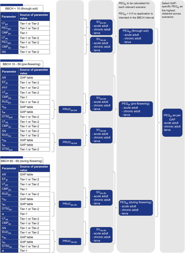
Visual interpretation of PEQdi derivation for Tier 1 and for Tier 2 exposure assessment
5.6. Exposure assessment for the screening step
As described above in this chapter, the exposure assessment for the dietary route of exposure is a complex process, involving several steps and numerous parameters. Therefore, the WG has formed a simplified method for the derivation of PEQdi values. This screening PEQdi can be used in the combined risk assessment (see Chapter 7). Applying this screening is an option, but not mandatory and can only be used as far as the cumulative application rate (AR x n) is not higher than 4.5 kg/ha (for further details on that limit are included in section 5.6 of the supplementary document). The method for PEQdi derivations for the screening step is a simplified version of the Tier 1 method as described in Section 5.1.2, resulting in conservative exposure estimations compared to Tier 1. In the simplified model for the preflowering contamination and for the during‐flowering contamination models, application rate (AR; g/ha) and the number of applications (n) – as described in Section 5.1.2 – has to be combined with a constant in the following way:
| (15) |
where B is a constant that depends on the risk case and the application method as presented in Table 22 below.
Table 22.
The values of constant B (μg/bee or μg/bee per day or μg/larva/developmental period) for each risk case by application methods
| Category for the risk assessment | Risk case | Constant B to be used for downward spray and granular application | Constant B to be used for sideward/upward spray application | Constant B to be used for seed treatment |
|---|---|---|---|---|
| Honey bee | Acute adult | 6.4 | 9.0 | 1.08 |
| Chronic adult | 6.2 | 9.0 | 1.04 | |
| Larva | 7.2 | 9.2 | 1.21 | |
| Bumble bee | Acute adult | 10 | 13.7 | 1.67 |
| Chronic adult | 9.6 | 13.3 | 1.62 | |
| Bombus terrestris larva | 33.7 | 48.5 | 5.66 | |
| Solitary bee | Acute adult | 0.70 | 0.94 | 0.12 |
| Chronic adult | 0.67 | 0.90 | 0.11 | |
| Osmia bicornis larva | 38.2 | 57.5 | 6.41 | |
| Osmia cornuta larva | 47.2 | 68.8 | 7.93 |
Due to the simplifications applied, this method results in more conservative PEQdi values for all situations which would be calculated by the models for preflowering contamination and/or for the during‐flowering contamination. Further details on the considered simplifications, the derivation of the exposure model for the screening step (equation 15) and the derivation of the constant values are reported in Section 5.6 of the supplementary document.
As regards the through‐soil contamination, single default PEQdi values are available (sum of the Tier 1 SVs), which are independent of the GAP. The values are included in Table 23, below.
Table 23.
The PECdi values (μg/bee or μg/bee/day or μg/larva/developmental period) relevant for scenarios where the through‐soil contamination model is to be applied
| Category for the risk assessment | Risk cases | PEQdi |
|---|---|---|
| Honey bee | Acute adult | 0.530 |
| Chronic adult | 0.500 | |
| Larva | 0.542 | |
| Bumble bee | Acute adult | 0.541 |
| Chronic adult | 0.511 | |
| Bombus terrestris larva | 1.357 | |
| Solitary bee | Acute adult | 0.044 |
| Chronic adult | 0.041 | |
| Osmia bicornis larva | 0.993 | |
| Osmia cornuta larva | 1.783 |
The next step is to compare the PEQdi values calculated by applying equation 15 with the PEQdi values reported in Table 23, above. For each risk cases, the highest of the two PEQdi values has to be considered in the risks assessment for the screening step.
As regards to the screening step for the contact exposure, the PEQco as calculated for Tier 1 has to be considered, but without the EFco parameter; i.e. the simplified model is:
| (16) |
The units of the parameters are the same as described in Tier 1, above (section 5.1.1).
6. Effect assessment in lower tiers
As explained in Chapter 3, the aim of the effect assessment is to identify the relevant hazard parameters or ‘effect endpoints’ to be used together with the PEQj, for estimating the levels of risk.
In the lower tier level, the hazard is defined by the dose–response curve (hereafter DRCj) investigated in standard laboratory tests. Once again, the suffix j indicates one of the four risk cases (i.e. acute oral, acute contact, chronic, larvae).
The WG considered that the use of the full dose–response relationship would improve upon the previous methodology, which relied on single effect point estimates (e.g. NOED, LD50) without an explicit consideration of the predicted level of effect triggered by a different exposure level. Therefore, the effect endpoints are the combination of the chosen dose–response model and the values of its parameters for each specific DRCj. Nonetheless, in some parts of the guidance document, the LD50 is still used (particularly for comparison purposes). Note that in this chapter the generic acronym LD50j is used for all risk cases. Nonetheless, when referred to chronic dietary experiments, this should be interpreted as an LDD50.
The choice of the dose–response to be used is limited to four models (see supplementary document), i.e. those included by the most recent BMD guidance document (EFSA Scientific Committee, 2022) in the family 1a for quantal endpoints. The limitation to models included in family 1a is due to the need to shift each DRCj (see Section 6.5 and Chapter 8) on the dose axis, by applying a multiplication/division factor on one model parameter, without changing the shape of the DRCj on a log‐scale. While acknowledging that the model averaging approach proposed by the most recent BMD guidance document (EFSA Scientific Committee, 2022) would be the most robust choice from a statistical perspective, the WG considered that the most traditional model selection approach proposed in the previous version of the BMD guidance document also presents some advantages. In particular, selecting a specific model whose parameters have a straightforward interpretation presents clear advantages in terms of communication. Therefore, the WG considered this deviation from the latest BMD guidance document acceptable.
In order to use appropriate hazard parameters in the risk assessment, risk assessors should carefully consider various aspects, which are presented in the following sections. These are:
Definition of hazard parameters in experimental studies indicated by the legal requirements (Section 6.1);
Dealing with equivalent studies performed with the same substance and the same species (Section 6.2);
Derivation of a surrogate dose–response beyond the tested range (Section 6.3);
Consideration of time‐reinforced toxicity (Section 6.4);
Extrapolation of the hazard parameters between species (Section 6.5).
6.1. Definition of hazard parameters in experimental studies indicated by the legal requirements
6.1.1. Legal requirements
Under Regulation (EC) No 1107/2009, the data requirements are set in Regulation (EC) No 283/2013 (for active substances) and Regulation (EC) No 284/2013 (for PPPs). For bees, they are described in point 8.3 and 10.3, respectively.
More specifically, Regulation (EC) No 283/2013 requires that:
Acute oral and contact toxicity to bees is tested where bees are likely to be exposed (8.3.1.1);
Chronic toxicity to bees is tested where bees are likely to be exposed (8.3.1.2);
Honey bee brood study shall be conducted to determine effects on honey bee development and brood activity, unless exposure of brood is not possible. The bee brood test shall provide sufficient information to evaluate possible risks from the active substance and the plant protection product on honey bee larvae (8.3.1.3).
The test protocols are listed in the European Commission Communications to the data requirements. It is noted that at the time of the publication of this guidance no international agreed protocols for bumble bees and solitary bees are listed. In addition, some test methods and guidance currently included are not recommended in this document. However, an update of these communications is ongoing and further clarifications need to be addressed by European Commission.
Nonetheless, in order to get a more robust risk assessment, any dossier should, in principle, contain experimental tests for all bee groups that are required for the relevant uses, depending on the problem formulation (see Chapter 4). As a general rule, these tests should be performed according to the standard guidelines. At the time of the publication of this guidance, OECD test guidelines are only available for honey bees and bumble bees (see Table 25). However, applicants could use other existing protocols (pending validation and adoption of new test guidelines, see overview in Table 25) to complement the data package.
Table 25.
Overview of the current availability of standard test guidelines
| Test type | Honey bee | Bumble bee | Solitary bee |
|---|---|---|---|
| Acute oral test | OECD Test Guideline No. 213 (OECD, 1998a) | OECD Test Guideline No. 247(OECD 2017c) | Standard test methods not yet available 1 |
| Acute contact test | OECD Test Guideline No. 214 (OECD, 1998b) | OECD Test Guideline No. 246 (OECD, 2017b) | Standard test methods not yet available 2 |
| Chronic test | OECD Test Guideline No. 245 (OECD, 2017a) | Standard test methods not yet available | Standard test methods not yet available |
| Test on larvae | OECD Guidance Document No. 239 (Repeated Exposure) | Standard test methods not yet available | Standard test methods not yet available 3 |
Draft version available for Osmia species (Roessink et al., 2019).
Draft version available for Osmia species (Roessink et al., 2018).
Proposal for a test protocol available for two Osmia species (Claus et al., 2021).
Within this guidance document, a methodology for conservatively – in most cases – extrapolating from honey bees to the other bee groups is presented (Section 6.5).
Relevant data from the scientific peer‐reviewed open literature on the active substance and formulated products shall be submitted together with the standard studies. Thus, additional laboratory toxicity data on bees may be available. When conducting a systematic literature search, the search strategy can be conducted following two general search approaches as recommended by EFSA (2011). The relevance and reliability of all available studies should be considered for the overall selection of endpoints, including information that is relevant for endpoint setting that may come from public literature and non‐standard guideline studies.
According to Regulation (EU) No 284/2013, when the toxicity of the PPP cannot be reliably predicted from the active substance data, studies (acute oral and contact, chronic, honey bee brood) performed with the PPP are required (from Section 10.3.1.1–10.3.1.3). In the case of mixtures i.e. PPP where the active substance is always intended to be used together with a safener and/or synergist and/or in conjunction with other active substances, toxicity of the mixture cannot be predicted based on the data of the active substance; therefore, data on PPP‐mixtures are always required (see Table 24). For the risk assessment of PPPs containing more than one active substance, see Chapter 12.
Table 24.
Summary of the data requirements for the active substance and the formulated products
| Tier 1 study type | Study with active substance (where bees are likely to be exposed) required? | Study with formulation required? | |
|---|---|---|---|
| Formulation with one active substance | Formulation with more than one active substance | ||
| Acute oral | Yes | Yes (a) | Yes |
| Acute contact | Yes | Yes (a) | Yes |
| Chronic oral toxicity to adults | Yes (c) | Pending on the comparison between acute studies (b) | Yes |
| Toxicity to larvae | Yes (c) | Pending on the comparison between acute studies (b) | Yes |
Acute studies with the formulation can be waived when the toxicity can be predicted on the basis of the active substance (e.g. when the formulation consists of the active substance only, or of the active substance in water).
Generally, a study with the active substance will be sufficient; however, if there is an indication from the acute oral study that the formulation is more toxic than the active substance, then the formulation should be tested. In determining whether there is a difference then the endpoints should be expressed in terms of active substance. If the acute formulation endpoint expressed as active substance is more toxic by at least a factor of 3 than the acute endpoint for the active substance, then it can be assumed that the formulation is of greater toxicity and hence chronic and larval testing should also be carried out using the formulation. If the difference is less than a factor of 3, then testing adult chronic and larval toxicity with the active substance is sufficient.
In case of poorly soluble substance, a single study on the formulated product might also be appropriate as surrogate if higher solubility levels are expected with the formulated product under the test conditions.
As further interpretation of the legal requirements, for PPPs containing only one active substance, at least acute (contact and oral) studies are required for both the active substance and the PPP, as this is the basis for a toxicity comparison between the active substance and the PPP. A chronic toxicity study and a honey bee brood study with the PPP can be waived, if, based on the comparison between acute toxicity studies, the PPP results in a comparable or lower toxicity than the active substance. A ratio of three should be used for the investigation of potential higher toxicity of the PPP based on the acute toxicity endpoints. Therefore, if:
LD50ac (a.s.)/LD50ac (PPP10) > 3 ➔ all the data requirements must be fulfilled by providing, in addition to the acute data, chronic and brood data for both the active substance and the PPP;
LD50ac (a.s.)/LD50ac (PPP 10 ) ≤ 3➔ no further data on the PPP are required.
For considerations concerning (1) availability of several equivalent tests carried out with the same species and the same test item and (2) uncensored LD50 values, please see Sections 6.2 and 6.3, respectively. Further consideration of the comparison between active substance and representative PPP are reported in Section 6.7.1.
6.1.2. Toxicity studies
Many OECD guidelines and guidance documents for bee testing have become available in recent years or are under development (see Table 25).
For all standard tests on adult honey bees and bumble bees (ring tested on Bombus terrestris and Bombus impatiens), the main endpoint is mortality. However, sublethal effects are also recorded (see Chapter 9).
Though not required in all test guidelines, the WG highly recommends always performing analytical verification of the exposure during the test.
The declared purpose of all these standard test guidelines is the derivation of a reliable LD50 expressed as mass of a.s./bee (a LDD50 expressed as mass of a.s./bee per day for chronic tests). Generally, the range of concentrations used in the tests should be wide enough to yield mortality effects that span from very low to high (i.e. > 50%), in order to derive a reliable LD50. This is often enough to derive a reliable full dose–response as well.
OECD ‘unclassified’ guidance document No. 239 (OECD, 2016) is available to address the data requirement for honey bee brood. The test exposes young honey bee larvae in artificial cells for 4 days via treated food in/on which they lie and follows them up to and including the moment of adult emergence from the pupae. The main recorded endpoints are mortality at larval and pupal stage and emergence, which can also be considered a proxy for lethal effects.
Guidance document No 239 should be used instead of an earlier publication, OECD guideline 237 (OECD, 2013), which only exposes the larvae for a single day and ends at pupation.
Test recommendations for larvae other than the honey bee are not available and the current data requirements specifically address only honey bees. In the OECD Guidance Document No 239, it is specified that ‘The method aims at the determination of a No Observed Effect Concentration/Dose (NOEC/NOED) and, if data allows, EC50/ED50’. Indeed, even in EFSA (2013), the focus was on deriving a NOED. In the context of this guidance document, the derivation of a NOED is no longer relevant, as the risk assessment is based on the dose–response relationship. Ideally, in order to appropriately describe the full dose–response, any larval test should be conducted with doses triggering several effect levels, with at least one being greater than 50%. Nonetheless, in the risk assessment scheme proposed in this guidance document, any predicted exposure PEQj equivalent to a dose causing effects > 10% at the individual level will immediately trigger a high risk at the lower tier of the assessment (see Chapter 8). In consideration of this, a reliable description of the lower part of the dose–response would still be sufficient for a substance‐specific hazard characterisation (see Section 6.3). Thus, the change in the endpoint is not anticipated to entail any modification of the existing OECD Guidance Document.
For experiments carried out as limit tests, a study‐specific DRC cannot be obtained, and a surrogate should be used (see Section 6.3).
It is acknowledged that tests submitted in dossiers may have been performed using a draft version of a guideline that has since been superseded by a final version. It is up to the risk assessor to determine whether such test is still acceptable for use in the risk assessment or if a new test should be performed. This will be determined on a case‐by‐case basis and may depend, among other things, on:
the timing of the evaluation compared to the guideline update, acknowledging that studies are generally performed before submission of a dossier;
the changes made to the specific guideline, e.g. are the deviations from the final guideline expected to have severely impacted the outcome of the test?; and
the importance of the endpoint in the overall risk assessment, e.g. are higher tier tests available that cover the first‐tier endpoint?
Similarly, the reliability of endpoints from draft test guidelines which have not been finalised by the OECD should be carefully considered in light of potential scientific concerns and relevance to the proposed risk assessment scheme.
6.2. Combining equivalent studies performed with the same test item and the same species
Often, multiple equivalent tests are available e.g. more acute contact tests with honey bees and a certain test item. Differences between the results of these tests are likely driven by experimental variability, thus averaging is generally proposed.
It must be noted that this averaging procedure is not recommended between tests carried out with different test items (e.g. one active substance and a formulation). On the contrary, if multiple equivalent tests are available with the active substance or with a formulation, averaging among tests performed with the same test item is recommended before checking whether the formulation shows higher toxicity compared to the active substance (see Sections 6.1 and 6.7).
Whenever multiple equivalent studies are available, the data sets can, in principle, be merged before fitting any dose–response model. This is in line with previous guidance documents (e.g. EFSA, 2009), as it is expected that any set of equivalent experiments is carried out according to the same protocol. If the survival in the control differs among the experiments, it may be appropriate to transform the data using a corrected survival before merging.
In some instances, the outcome of different experiments may be considerably different, and fitting a single model to a merged data set will lead to a large uncertainty. In such cases, it is worth exploring whether the recorded difference is due to any known external factor, or whether the experiments differ in their level of reliability. Excluding data sets in consideration of these aspects requires a case‐by‐case decision.
6.3. Derivation of a surrogate dose–response beyond the tested range
For substances with low toxicity and ‘difficult’ substances (e.g. with low solubility), it is often the case that the highest tested dose or the ‘limit dose’ shows an effect < 50%. In this event, the LD50 is often referred as a right‐censored value (e.g. LD50 > 100 μg a.s./bee). In the past, the lower bound of the endpoint was used in the risk assessment. This approach overestimates the actual toxicity and might bias the risk assessment of substances with low toxicity.
In these cases, the experimental data do not always allow describing a dose–response. However, a surrogate dose–response can still be derived by making some conservative assumptions.
In the context of the proposed risk assessment scheme, the most important part of the dose–response is the one below the LD10. This is because an effect higher than 10% would immediately trigger a concern of high risk. Thus, the use of the methodology proposed in this section is mandatory for limit test experiments (i.e. tests with a single treatment dose) and dose–response experiments when the maximum dose did not trigger an effect > 10%. In every other case, the data may be sufficient to describe at least the left part of the dose–response, in which case the use of a surrogate is not needed.
Whenever data do not allow estimating even a partial dose–response relationship (at least up to 10% effect), the choice of the model for a surrogate dose–response curve is completely arbitrary. To maintain a standardised approach, for the present guidance, it was chosen to rely on log‐logistic dose–response models. When dealing with survival data, these are mainly defined by a slope and the LD50 (corresponding to the inflection point, see supplementary document section 6 for further details).
For any specific dose x assuming a shallower slope will result in the prediction of higher effects for any dose < x. In the risk assessment scheme proposed in this guidance document, any predicted exposure PEQj equivalent to a dose causing effects > 10% at the individual level will immediately trigger a high risk in the lower tier of the assessment (see Chapter 8). This means that underpredicting effects above 10% have no consequence on the outcome of the risk assessment. On the contrary, it is of utmost importance to ensure that a prudent approach is adopted when predicting effects in the range 0–10%, as their combination will determine the outcome of the lower tier risk assessment (see Chapter 8).
As a conservative approach, a log‐logistic dose response with a default slope of 1.43 can be used whenever a specific value cannot be reliably determined from the experimental data. This corresponds to the 10th percentile of the slope distribution based on an analysis of log‐logistic dose–response curves obtained from a large number of substances (see Section 6.3 in the supplementary document).
Once the slope is fixed, a surrogate LD50 can be derived by multiplying the highest (or single) tested dose to an appropriate extrapolation factor, depending on the observed effect. This is conceptually similar to the extrapolation factors for LD50 reported in the guidance document for birds and mammals (EFSA, 2023). For sake of simplicity and conservativeness, the observed effects are categorised into five effect intervals, with the higher end being used for derivation of extrapolation factors.
As significant differences among slopes were not recorded between groups of substances and test types, a unique set of extrapolation factors (reported in Table 26) can be applied to all kinds of tests.
Table 26.
Extrapolation factors for different intervals of effect
| Effect observed (corrected mortality) at the highest tested dose | Effect < 10% | 10 ≥ effect < 20% | 20 ≥ effect < 30% | 30 ≥ effect < 40% | 40 ≥ effect < 50% |
|---|---|---|---|---|---|
| Extrapolation factor to be applied to the highest tested dose | 4.6 | 2.6 | 1.8 | 1.3 | 1 |
To summarise, whenever not even a partial dose–response can be derived from the experimental data, a surrogate log‐logistic dose–response can be derived by:
-
–
Using a worst‐case default slope = 1.43;
-
–
Using the appropriate extrapolation factor to derive a surrogate LD50.
For example, considering a limit test where the control mortality was equal to 3% and the mortality in the only treatment level (100 μg a.s./bee) was 9% (corrected mortality = 6.2%). As the (corrected) effect of the treatment was below 10%, the extrapolated LD50 should use the factor of 4.6 from Table 23, thus: surrogate LD50 = 100 μg a.s./bee × 4.6 = 460 ug a.s./bee. This value together with the worst‐case slope of 1.43 is sufficient to predict the effect of any dose x using the equation of the log‐logistic model (see Chapter 6 of the supplementary document).
6.4. Time‐reinforced toxicity (TRT)
A substance shows time‐reinforced toxicity (TRT) when its toxic effects from exposure to low doses for a long period of time are higher compared to effects from exposure to higher doses for a short period of time (i.e. its toxic effects are reinforced by exposure time). Note that this phenomenon was called ‘accumulative toxicity’ in the EFSA (2013).
The studies required by Regulation (EC) No 283/2013, 8.3.1 and Regulation (EC) No 284/2013, 10.3.1 are limited to studies assessing the effects from fixed exposure durations (acute and chronic). This approach is valid when toxicity is mainly dependent on the dose. However, for substances which show TRT, the impact of low doses may be underestimated if the exposure period tested in the laboratory is shorter than the environmentally relevant length of exposure. Therefore, the WG considered it necessary to always assess whether a substance shows TRT.
The assessment strategy for TRT included in this guidance document (see Chapter 8) is based on the results of the honey bee chronic toxicity study according to OECD guideline 245 (OECD, 2017a). Therefore, in principle, no additional studies need to be performed for the TRT assessment.
The 10‐day duration of a chronic study according to OECD 245 has been criticised as being too short to address longer exposure to low doses. However, an analysis performed by the WG has shown that data from a 10‐day study can be used to reliably predict the toxicity for a longer exposure period (please refer to Section 5 of Annex G to the supplementary document for details). It should, however, be noted that at least some mortality should be observed in the study for it to be useful for the TRT assessment (i.e. the level of mortality reached at the end of the test period should be high enough to allow the calculation of a LDD50 or LDD25 value for at least day 10; refer to Chapter 8 for further details). Therefore, the doses tested should be carefully considered.
If a conclusion on the occurrence of TRT cannot be drawn based on the available 10‐day chronic lethal toxicity study, a study specifically designed to investigate TRT can be performed. For the design of such a study, there are different options, as detailed in Chapter 8.
For substances with a low toxicity to bees, additional testing might not be necessary: if mortality is ≤ 10% at the end of the test for any dose ≥ 100 μg a.s./bee/day, an assessment of TRT is not required. For substances of low solubility, for which it is not possible to reach a test dose of 100 μg a.s./bee per day, potential solutions are described in Chapter 8.
Whenever a substance shows TRT behaviour, the life span dose–response obtained from the TRT assessment substitutes the 10‐day dose–response obtained directly from the chronic testing with honey bees.
Note that the possibility to waive a chronic study and a honey bee brood study with the PPP on the basis of a comparison between acute studies with both the active substance and the PPP (see Section 6.1.1) is maintained when a substance shows TRT behaviour.
6.5. Extrapolation between species
The lack of toxicity data for bumble bees and solitary bees makes it difficult to assess the risk of pesticides for these bee groups. The issue of how LD50s differ among bee species has been investigated from different perspectives, in order to determine suitable extrapolation factors. Details about the analysis underlying this section are available under Section 6.5 of the supplementary document.
The available data allowed a meaningful comparison of acute, mostly contact, tests; nevertheless, this was not the case for other types of studies due to the lack of standardised chronic and larvae tests for species other than Apis mellifera. Therefore, in the absence of suitable alternatives, and until better data become available, the WG recommends that the derived factors are applied to all types of tests with adult bees, despite being uniquely derived from the acute (mainly contact) tests.
The availability of bee weight measured in some ecotoxicity experiments allowed establishment of a generic (substance‐independent) relationship between LD50 and bee weight. Thus, collection of adult bee weight data for a representative number of European bee species (~ 10%) allowed calculation extrapolation factors from standard species to smaller bumble bees and solitary bees, in order to protect at least 95% of European species with 95% confidence. The WG has considered this to be a very conservative approach that can be revised if more information becomes available. These factors are referred to as ‘Toxicity extrapolation factors’ (Tef) and are reported in Table 27 for standard species.
Table 27.
Toxicity extrapolation factors (Tef). Standard LD50j should be divided by these factors to obtain an estimate of an LD50,j protective of 95% of the species in the group
| Test species | Tef for extrapolation to | |
|---|---|---|
| 5th percentile bumble bee weight | 5th percentile solitary bee weight | |
| Standard honey bee adult (A. mellifera worker) | 2.4 | 171 |
| Standard bumble bee adult (B. terrestris (a) worker) | 6.6 | – |
|
Standard solitary bee adult (O. bicornis ♀) (O. cornuta ♀) |
– – |
144 307 |
|
Standard honey bee larva (A. mellifera worker) |
1.0 (b) |
1.0 (b) |
OECD test guidelines No 246 and 247 were also ring tested with B. impatiens. If data are available with this species, both Tef and food consumption values should be recalculated based on the appropriate body weight. For Tef, the formula is available in the supplementary document under Section 6.5.4. Camp et al. (2020) reported an average weight of 178 mg for B. impatiens.
Tef not meant to address the 5th percentile species in terms of weight, but rather Bombus terrestris for bumble bees and Osmia species for solitary bees, i.e. species used to estimate the exposure levels to bumble bees and solitary bees.
The Tef values only refer to the hazard definition, so that smaller bees would be characterised by smaller LD50 (higher hazard). However, as explained in Chapter 5, exposure estimates are also dependent on body weight (see Section 5.3.5) and body surface area (see Section 5.2.3), so that smaller bees are characterised by lower exposure.
For larvae, no suitable information is available to relate either the LD50 or the predicted exposure levels to bee size, so an extrapolation equivalent to the one performed for adult bees is not possible. As explained in Chapter 5, exposure estimates are based on Bombus terrestris for bumble bees and Osmia species (O. bicornis and O. cornuta) for solitary bees. The larvae of these species are not significantly smaller than those of honey bees. As such, a Tef = 1 is proposed from honey bee larvae to bumble bees and solitary bee species (see Table 27).
Hence, the appropriate extrapolated LD50j for bumble bees and solitary bees is be derived from the following equation:
| (17) |
In most of the cases, the standard LD50j (which can, in some cases, be a surrogate LD50j) is derived for honey bees. Nevertheless, if data are available on other standard species, those should be used in the derivation of the extrapolated LD50j for their specific bee group.
The extrapolation factors presented in this section are estimated from the relationship between LD50 and bee weight. Nevertheless, weight is not the only driver of the LD50, as demonstrated from another analysis which investigated generic ‘intrinsic’ sensitivity of various species (see Section 6.5.3.7 of the supplementary document). Among those, A. mellifera was the most intrinsically sensitive, which gives confidence that the extrapolation factors from this species are likely protective, despite some remaining uncertainty.
The whole analysis focussed on finding general patterns across substances. In some particular cases, a certain species may be more sensitive to a substance due to very specific toxicodynamic processes (Hayward et al., 2019). Nevertheless, at the current stage, this cannot be predicted or accounted for in the risk assessment, as the knowledge on this topic is still very limited.
Almost no information is available in the literature concerning the shape (i.e. the slope) of dose–responses for bees other than honey bees. Nevertheless, there is no particular indication that the slope of the dose–response, which is mainly driven by toxicokinetic and toxicodynamic aspects, should vary significantly among bees. In consideration of this, as a pragmatic approach, it is suggested that the DRCj obtained from tests carried out with honey bees should be simply shifted on the doses axes by a factor equal to the Tef when describing homologous effects to other bee groups.
On a practical level, this means that the model and the parameters of the DRCj used for honey bees will remain the same, except that the parameter expressing the inflection point should be divided by the appropriate Tef (e.g. DRCch obtained from chronic tests with honey bees may be used for determining the chronic dose–response of the other bee groups simply by dividing one parameter by the Tef values in the first line of Table 27).
If a dose–response is available from tests with (standard) bumble bees and/or solitary bees, this should be used as a starting point to derive the representative DRCj for their own group of bees, following the same procedure illustrated above, but using Tef values from lines 2 and 3 of Table 27.
6.6. Implications of the time course of effects on exposure assumptions
In some cases, the initial exposure is that causes most of the effects, which are expressed immediately, even during constant chronic exposure. This would normally be the case for substances with fast kinetics, under the assumption of individual tolerance. Expressing the exposure in terms of time‐weighted average for these substances may significantly underestimate the effects under the time‐variable exposure expected in the field. Thus, when it is demonstrated that the effects observed are largely due to the level of initial exposure rather than to the exposure duration, the only exposure that matters is the acute one.
Nonetheless, combining the effects due to chronic and acute dietary exposure means, in these cases, counting the same process twice. Thus, when the effects in the chronic test are expressed over a short period, the acute dietary risk case is excluded from the overall estimation of the risk (Section 7.1.3), while the chronic risk case is determined by the 10‐day chronic DRC and the acute exposure level.
Effects which occur only due to a short exposure window despite chronic exposure are the opposite of effects resulting from the phenomenon of TRT. Indeed, in one case the effects are driven by the initial exposure and exposure time has limited influence, while in the other case the exposure time is the main determinant of the effects. Thus, if TRT properties have not been ruled out for a substance (including those substances for which no effects were seen in the chronic test), no further check is needed. On the contrary, if a lack of TRT has been demonstrated, a further step must be taken in order to determine whether chronic exposure estimations are applicable.
The simplest way to check whether effects are expressed immediately after the initial exposure is to check the temporal trend of the LDD50. This operation can be easily done after fitting a chronic test data set to GUTS models (something that would anyway need to be done for ruling out TRT properties – see Chapter 8). If the LDD50 after 2 days and after 10 days are significantly different or present a ratio > 3, it can be concluded that the exposure time plays an important role in the overall expression of effect, and thus no modification of the standard time window w is needed (Figure 8).
Figure 8.
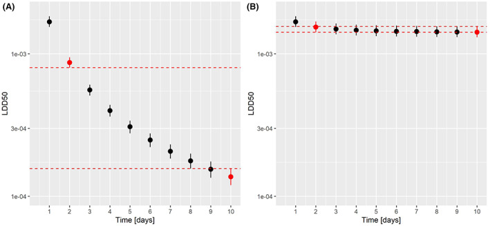
examples of different situations concerning the time course of effects. In panel A, full expression of effects depends on the exposure time. Uncertainty ranges of the LDD50 at 2 and 10 days are well separated (red dotted lines show lower limit of LDD50 at 2 days and upper limit at 10 days). In panel B, effects are almost entirely expressed after a short time. Uncertainty ranges of the LDD50 at day 1 and day 10 overlap. In such cases, the assumptions normally used for estimating chronic exposure are not appropriate
6.7. Summary of the selection of hazard parameters for the risk assessment
To select the appropriate DRC to be used for risk assessment for each group of bees and each risk case j, it is necessary to consider all the elements discussed in the previous sections.
Since standard test protocols are available for honey bees covering the different risk cases, these are generally considered as starting points to derive the hazard parameters for other bee species as well, in consideration of the inter‐species sensitivity. However, in some cases, tests with bumble bee (Bombus terrestis) and solitary bee (Osmia spp.) standard species will also be available and should be used as a reference for the group of bees they belong to.
6.7.1. Hazard parameters for the risk assessment of honey bees
To select the representative DRCj for any test item (either an active substance or a PPP containing one active substance) it necessary is to consider all the available data and go through several steps. The procedure is summarised in the following steps and figures.
Step 1
When multiple equivalent honey bee tests with the test item are available, an attempt to merge the data sets should be made before fitting any dose–response model (Section 6.2). When the outcome of different experiments is considerably different, it is worth exploring whether the recorded difference is due to any known external factor or whether the experiments differ in their level of reliability. Selecting or excluding data sets in consideration of these aspects requires a case‐by‐case decision.
However, if none of the available tests allow the description of at least a partial dose–response covering effects at least as high as 10% (e.g. in the case of limit tests), a surrogate dose–response can still be obtained. This is achieved by applying the appropriate extrapolation factor to the maximum (or unique) tested dose in order to derive a surrogate LD50 (i.e. the inflection point of a log‐logistic model), as described in Section 6.3. A log‐logistic model with a worst‐case default slope of 1.43 should be used as a surrogate DRCj in these cases. Step 1 is illustrated in Figure 9.
Figure 9.
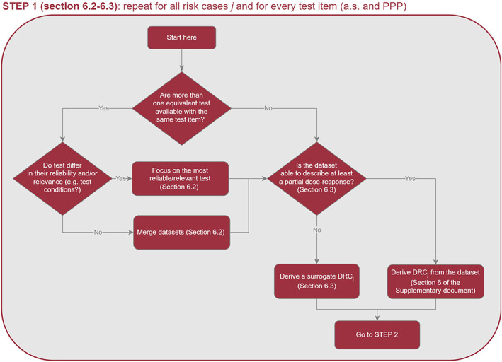
Flowchart illustrating the Step 1 of the process underpinning the selection of the hazard parameters for the risk assessment of honey bees. In this picture, tests are considered equivalent when they relate to the same risk case
Step 2
To identify the most appropriate DRCj for the honey bees risk assessment of active substances, it is necessary to consider the difference between the LD50 based on data for the representative PPP and the active substances (both expressed in terms of active substance). This step is not necessary if the representative PPP contains additional active substances. In such cases, the mixture assessment methodology should be followed (see Chapter 12). As explained in Section 6.1, if the LD50j for the PPP is more than a factor of 3 below that of the active substance, the PPP is considered more toxic. Hence, the hazard parameters related to the PPP must be selected for the risk assessment, including for the active substance in the context of its inclusion/renewal.
When one DRCj, between the active substance and the PPP is not a surrogate, this should be used for the risk assessment, unless this entails neglecting higher effects at comparable doses in one of the studies.11 When both active substance and PPP DRCj are surrogates, additional case‐by‐case considerations must be made concerning the mortality actually observed in the tests and the tested doses. For example, if the top/limit dose caused no mortality for either the PPP or the active substance, a comparison is not meaningful. In such cases, it would be appropriate to use the surrogate dose–response obtained from the highest tested dose (expressed as active substance) for the risk assessment.
This comparison is normally performed using acute data; however, if the PPP is acutely more toxic, chronic and larvae data with the PPP ‘should be provided and included in the comparison. In addition, if the PPP is more toxic, the risk assessment for the active substance should be based on the hazard parameters derived from tests with the representative PPP. For poorly soluble substances, chronic and larval studies may be carried out uniquely with the formulated product if higher solubility levels are expected with the formulated product under the test conditions. In such cases, the DRCj derived with the formulated product would be considered (as a surrogate) for the active substance. Step 2 is illustrated in Figure 10.
Figure 10.
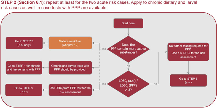
Flowchart illustrating the Step 2 of the process underpinning the selection of the hazard parameters for the risk assessment of honey bees. Note that the comparison of the LD50j between active substance and PPP entails additional consideration in case of surrogate DRCj (see text)
Step 3
The selection of hazard parameters for the chronic risk assessment of honey bees should take into account whether the active substance (and the PPP, if this is triggered at the Step 2) shows time‐reinforced toxicity (see Section 6.4 for the general concepts, Chapter 8 and Annex G of the supplementary document for more detailed explanations). If this is the case, the life‐span dose–response should substitute the 10‐days chronic dose–response. Furthermore, when this is the case, an additional risk assessment for winter scenario is triggered, using a life‐span dose–response for long‐lived winter bees (see Chapter 8). Step 3 is illustrated in Figure 11.
Figure 11.
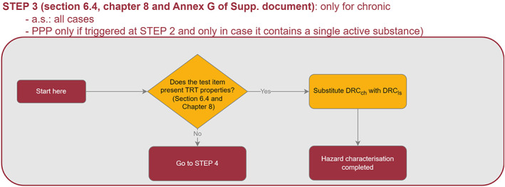
Flowchart illustrating the Step 3 of the process underpinning the selection of the hazard parameters for the risk assessment of honey bees
Step 4
When effects are driven mainly by the initial exposure and are expressed immediately, even in conditions of constant chronic exposure, estimating the exposure in terms of time‐weighted average may significantly underestimate the effects in the field (see Section 6.6). Thus, when it is demonstrated that the effects observed are largely due to the level of initial exposure rather than to the exposure duration, the chronic dietary risk case will combine the 10‐day DRC with the acute exposure estimate.
This situation will not occur if a substance presents TRT properties and/or if no effects are seen in the chronic test. The simplest way to check whether effects are expressed immediately after the initial exposure is to check the temporal trend of the LDD50 in a chronic test. If the LDD50 after 2 days and after 10 days are significantly different or present a ratio > 3, it can be concluded that the exposure time plays an important role in the overall expression of effect, and thus no need to deviate from the standard approach. If, on the other hand,, the chronic dietary risk case would make use of the acute dietary exposure, then the dietary acute risk case is excluded from the combination of effects in the risk assessment (Section 7.1.3). Step 4 is illustrated in Figure 12.
Figure 12.
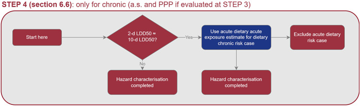
Flowchart illustrating the Step 4 of the process underpinning the selection of the hazard parameters for the risk assessment of honey bees. The effect of the exposure length is considered minor if the LDD50 after 2 days and after 10 days are not significantly different and present a ratio < 3
6.7.2. Hazard parameters for the risk assessment of bumble bees
For bumble bees, OECD TG 246 and 247 acute tests may be provided in the dossier with both active substance and representative PPP. In addition, relevant literature data may be available. The treatment of the hazard parameters (i.e. DRCj) from any available test with the standard species (Bombus terrestris and, less frequently, Bombus impatiens) should follow Steps 1–2 summarised in Section 6.7.1 for honey bees. Steps 3–4 are unlikely to be applicable until a standard chronic test with bumble bees is available.
However, since the bumble bee group includes many untested species (see Section 1), in order to cover the inter‐species differences, toxicity extrapolation factors (Tef) as described in Section 6.5 should be applied to obtain the relevant extrapolated DRCj.
In all cases when bumble bee data are not available (e.g. likely always for chronic and larval effects) the extrapolated DRCj should be obtained by applying the appropriate Tef to the DRCj selected for honey bees.
6.7.3. Hazard parameters for the risk assessment of solitary bees
For solitary bees, since standard tests are not yet available, the risk assessment should generally be based on hazard parameters previously selected for honey bees, with an extrapolated DRCj obtained after applying the appropriate Tef to the honey bee DRCj, as explained in Section 6.5.
However, when studies based on publicly available test protocols or draft OECD TG e.g. on O. rufa are available (likely for acute exposure only), they can be used to derive the hazard parameters for the solitary bee risk assessment. When this is the case, the DRCj from those studies could be used to obtain the extrapolated DRCj after applying the appropriate Tef.
6.8. Options for refinement
As possible refinements of the hazard, the WG considered the use of two approaches when equivalent tests on different species are available for the same substance, namely:
The geometric mean approach;
The species sensitive distribution (SSD) approach.
The WG highlighted that the species commonly tested are limited to A. mellifera, B. terrestris and Osmia spp. Tests with these species are used for separate risk assessments for honey bee, bumble bee and solitary bee, respectively. Any merging of data (either geometric mean or SSD) between these species is, therefore, not appropriate.
Furthermore, the hazard characterisation proposed in this guidance document relies on dose–responses, rather than point estimates. Thus, any combination of LD50 via either geometric mean or SSD would still not be sufficient to derive a combined DRCj – as this would mean combining different DRC based on different models and characterised by a different shape. Nonetheless, some relevant considerations are given in the next paragraphs.
If studies are available with multiple species belonging to the same bee group, the geomean approach could in principle be used to combine LD50 values after having applied the appropriate Tef to each of them. This would give an estimate of the variability of the ‘intrinsic’ sensitivity among species, once the expected contribution due to the bee weight has been removed. It is anticipated that this approach would not provide any significant change in the hazard assessment, unless the generic influence of weight on the LD50 used in this guidance (see Section 6.5) is significantly altered for the specific substance being investigated.
Similarly, in principle, if at least five species for a group (e.g. five solitary bee species) are tested and their body weight is sufficiently representative of the weight range of all bees in a group (e.g. from ~ 5 to ~ 130 mg for solitary bees, from ~ 100 to ~ 500 mg for bumble bees) or it is proven that body weight is not a significant driver of the hazard definition, the SSD could be a valid approach. In such cases, the HD5 (Hazardous Dose for 5% of the species) could be used as a representative LD50j for the group. However, the main practical issues preventing its use are the lack of standardised testing guidance for a sufficient number of species and the lack of agreed methods for combining other features of the DRCj.
When taken together the lack of standardised test guidelines for many species and the general lack of knowledge on inter‐species variability in the dose–response, mean that the WG cannot currently recommend the use of either the geomean or the SSD approach for bees. Nevertheless, for the time being, hazard information for multiple species could be considered in a weight of evidence, acknowledging that increasing the current level of knowledge would certainly improve the accuracy of the risk assessment in future.
7. Lower tier risk assessment
In line with the principles of the tiered risk assessment approach, the aim of the proposed methodology is to implement the agreed SPG in the lower tier risk assessment, resulting in a conservative assessment which simultaneously identifies active substances of concern while excluding the substances of least concern from further evaluation.
The suggested approach leaves behind the paradigm of evaluating the single endpoints separately and follows the rationale of combining a precise calculation of individual level effects with an extrapolation from individual to colony/population levels, and the aggregation of effects of a PPP on separate endpoints using the concept of response addition. This calculation method considers that in real life, PPPs can affect a honey bee or bumble bee colony or population of solitary bees by different routes of exposure (see Section 1.4). Here, instead of proposing empirical safety factors (i.e. trigger values) for assessing the risk of single exposure routes separately, this approach combines the predicted effects in a more mechanistic concept. This is much closer to the risk to bees of PPPs in the field and it is in line with the defined SPG, where the attribute dimension is the colony/population (see Chapter 1). The predicted effects following the exposure to a PPP at colony/population levels can then be directly compared to the SPG for bees. Since an SPG has been agreed for honey bees only, this means that the predicted effects will be compared to the agreed value of 10% of colony size reduction, which will be used as trigger for honey bees.
Practically, the proposed procedure for a ‘combined risk assessment’ is composed of three consecutive steps:
Quantification of the effects at the individual level for each risk case based on standard laboratory ecotoxicological studies, and exposure estimates;
Extrapolation of the individual level effects to colony/population level effects for each risk case;
Combination of effects for all risk cases into a single predicted effect at the colony/population level.
These steps are described in the following section. The proposed methodology is suggested for use for all bee types, including honey bees, bumble bees and solitary bees, despite the fact that for bumble bees and solitary bees a threshold of acceptable effect was not defined.
7.1. Step‐by‐step explanation of the lower tier approach for honey bees
7.1.1. Step 1: quantification of effects at individual levels
In this step, a dose–response curve (DRCj) is defined for each relevant bee type and life stage, which is used together with the relevant predicted exposure quantity (PEQj) to calculate the predicted effect at the individual level. This result describes the relationship between exposure to a PPP and the mortality and can be used to indicate the probability of death after exposure to a specified quantity of the PPP.
As explained in Chapter 6, the dose–response used in this guidance document is limited to four non‐linear models. A non‐linear dose–response relationship allows a much more accurate calculation of effects as compared to linear dose–response relationships. In the years since the publication of the previous guidance (EFSA, 2013a,b), evidence has been collected that observed dose response data follow sigmoidal rather than linear dose–response relationships (see Section 6.3 and supplementary document Section 6.3).
Formally, the calculation of the predicted effect, in unit of percentage, is given by
| (18) |
where PIE is the predicted individual level effect following the application and exposure of a PPP, j refers to a risk case as assessed in an experimental test such as acute‐contact, acute‐dietary, chronic‐dietary or repeated‐dose‐larvae; DRCj is the dose–response function f; and PEQj is a realistic worst‐case exposure estimate for the respective exposure assessment Tier, which could be screening, or Tier‐1 or Tier‐2. The exposure estimate is defined as ecotoxicologically relevant exposure quantity, here the uptake of pesticide by individual bee per time unit (see Figure 13). It is represented by the dose indicating the predicted environmental exposure (PEQj) as well as the one in the ecotoxicological experiment. Both are given in the same unit, which is mass of a.s.·individual−1(·time−1, for the chronic dietary risk case).
Figure 13.
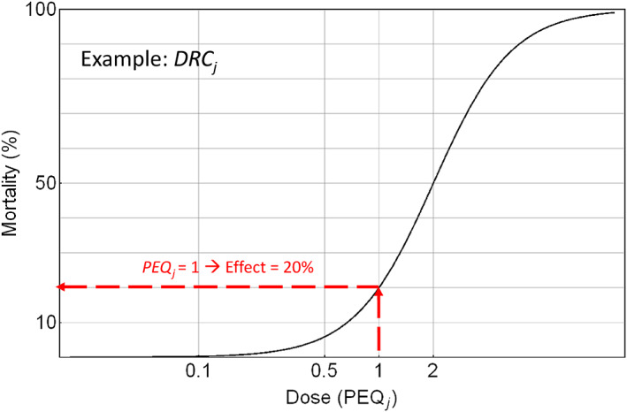
Graphical illustration of the proposed calculation for the effect on a specific endpoint using a non‐linear dose–response curve (DRCj). The resulting mortality (%) can be interpreted as probability of one individual to die on exposure to a certain dose, which can also be interpreted as a percentage of a cohort of individual bees to die after exposure to the identical dose
The PEQj represents the most relevant exposure estimation of the various possible sources of environmental exposures as defined by a proper problem formulation (see Chapter 4, overview in Table 28). The calculation of PEQj values is described in Chapter 5, while the definition of the required hazard parameters is in detail described in Chapter 6, including the determination of values for bumble bees and solitary bees, and the procedure if no suitable dose–response relationship can be derived.
Table 28.
Overview of exposure and the dose ‐response for the different life stages of honey bees
| Life stage | Category | Exposure | Hazard | ||
|---|---|---|---|---|---|
| Route | Duration | Quantification and time scale | Dose–response | ||
| Adult | Forager | Contact | Acute |
From contact exp. model; pesticide mass sticking on the forager after a single application |
Determined experimentally from the acute contact test. If it cannot be derived, a worst‐case surrogate is used (see Chapter 6). |
| Adult | Forager | Dietary (oral) | Acute |
Worst case between the two bee roles from dietary model; pesticide mass uptake per bee per day |
Determined experimentally from the acute oral test. If it cannot be derived, a worst‐case surrogate is used (see Chapter 6). |
| Adult | In‐hive (nurse) | ||||
| Adult | Forager | Dietary (oral) | Chronic |
Worst case between the two bee roles from dietary model; average daily pesticide mass uptake per bee during: 10 days (standard chronic assessment) – 27 days, i.e. the average lifespan of honey bee workers (for substance with TRT properties) |
Standard chronic assessment Determined experimentally from the chronic oral test. If it cannot be derived, a worst‐case surrogate is used (see Chapter 6). TRT assessment Determined via extrapolation from the chronic oral test. |
| Adult | In‐hive (nurse) | ||||
| Larvae | General worker | Dietary (oral) | Chronic (prolonged) |
From dietary model; average daily pesticide mass uptake per larvae during 5 days |
Determined experimentally from the larvae prolonged test/repeated exposure. If it cannot be derived, a worst‐case surrogate is used (see Chapter 6). |
When a substance has TRT properties, the risk should be evaluated for the entire honey bee lifespan for both the active (27 days) and the winter (182 days) period. Nevertheless, the winter scenario is a stand‐alone assessment, which does not follow all of the steps illustrated in this Chapter. See Section 8.2.2 for more details.
7.1.2. Step 2: extrapolation of the individual level effects to colony
In lower effect‐tier assessment, toxicity endpoints investigated in lab studies are expressed at levels of individuals. However, the SPG defines the relevant ecological entities as the colony for honey bees and bumble bees, and the population for solitary bees. To make the lower tier risk assessment compliant with the SPG, effects need to be extrapolated from individual levels to higher levels of biological organisation (i.e. colony or population). Since not every individual level effect might immediately propagate equally to colony levels and as there are feedback mechanisms influenced by environmental conditions, a reliable extrapolation from individual to colony levels for honey bees appears challenging. The impact of individual level effects on colony levels was therefore analysed by using the BEEHAVE model, using simulated colony level feedback mechanisms, and thereby allowing an analysis of this extrapolation between individual and colony effects under variable ecological conditions. The use of BEEHAVE is here not justified by a detailed analysis of the included processes, but based on an extensive literature review and comprehensive analyses of all available bee colony models, which resulted in the finding that BEEHAVE is the most suitable currently available choice (EFSA, 2021). In the absence of any other experimental or conceptual method for the extrapolation of individual to colony levels, besides the use of assessment factors, the WG assumes here that the extrapolations resulting from a dedicated use of the BEEHAVE model are appropriate. All analysed extrapolations (see Section 7.1.2 in the supplementary document) are based on the general consideration of a worst‐case exposure related to a certain risk case, here for larvae, foragers and in‐hive bees.
Overall, in the lower Tier risk assessment based on lethal effects, the extrapolation step assumes a conservative 1:1 propagation of individual to colony level effects for all experiments, i.e. using dietary and contact exposure, formally written as
| (19) |
where PCEj is the predicted colony level effect obtained from risk case j, expressed as percentage.
7.1.3. Step 3: combination of effects at the colony
In this third step, effects predicted for single risk cases are combined, based on the rationale that under real world conditions effects produced by different routes of exposure and on different life stages are adding up at the colony level, which is the ecological entity defined for the SPG. This rationale is based on the assumption that different bees are exposed acutely and chronically, via the diet or contact. The addition of responses to the single risk cases as estimated in step 1, and extrapolated to the colony level at step 2, is mathematically expressed by:
| (20) |
where PESPG is the overall predicted effect at the colony level, in units of % of colony size reduction, and the symbol Π means a multiplication of all terms from 1 to n. This value is directly compared with the SPG i.e. ≤ 10% colony size reduction for honey bees. The maximum effect is mathematically limited to 100%, independent of the number of considered endpoints. Neglecting the timing of single events in the response addition calculation is common for Tier 1 methods and a conservative assumption.
It is noted that the combined approach uses the worst‐case PEQj from the different scenarios, irrespectively of relevant timing of the scenarios.
In the Table 29 an example is presented to illustrate how the calculations will be performed to estimate the risk to honey bees at colony level by combining the different risk cases.
Table 29.
Example on how to estimate the risk to honey bees with the combined approach
| Honey bees Tier‐1 exposure | |||||
|---|---|---|---|---|---|
| Dietary | Contact | ||||
| Acute (da) | Chronic (dc) | Larvae (dl) | Acute (ca) | ||
| Exposure (Tier‐1) [μg/bee]a,b | PEQj | PEQda = 1.12 | PEQdc = 0.53 | PEQdl = 0.64 | PEQca = 2.28 |
|
Hazard parameters (DRC j ): Dose–response model (Mod) Inflection point (e)[μg/bee] (a) Slope parameter (b) |
DRCda Mod: log‐logistic e = 10.5 b = 1.84 |
DRCdc Mod: log‐logistic e = 6.75 b = 1.67 |
DRCdl Mod: log‐logistic e = 4.75 b = 2.24 |
DRCda Mod: log‐logistic e = 12.4 b = 2.23 |
|
| Step 1: Predicted individual level effect (PIE) | PIEda = 1.6% | PIEdc = 1.4% | PIEdl = 1.1% | PIEca = 2.2% | |
| Step 2: Predicted colony level effect (PCE) | PCEda = 1.6% | PCEdc = 1.4% | PCEdl = 1.1% | PCEca = 2.2% | |
| Step 3: combination of effects at colony level |
PESPG = 100·(1−(1−PECda/100)·(1−PCEdc/100)·(1−PCEdl/100)·(1−PCEca/100)) = 100·(1−(1–0.016)·(1–0.014)·(1–0.011)·(1–0.022)) = 6.2% |
||||
| PESPG i.e. ≤ 10% | Y (high risk excluded) | ||||
Units are mentioned for brevity as μg/bee, but they are in fact μg/bee per day for chronic and μg/bee per dev. Period for larvae.
7.1.4. Quantification of the contribution of a risk case to the overall predicted effect
There might be cases where the overall predicted effect at the colony level PESPG is dominated by a single risk case. Depending on whether or not a single risk case dominates the PEspg, different options for refinement can be used in the higher tier risk assessment (see Chapter 5). In order to assess the potential dominance, the contribution of one risk case on the overall predicted effect needs to be quantified. This cannot be done by simply building the ratio between a single risk case and the overall predicted effects, since the aggregation by response addition is not additive, but multiplicative. From the definition of the PESPG, a formula can be derived for the contribution of risk case j, named to the overall predicted effect
| (21) |
7.2. Implementation of the combined risk assessment in the tiered approach
As explained in Section 7.1 the quantification of individual effect (step 1 of the combined risk assessment) is driven by the PEQj from the exposure and by the DRCj for the hazard.
Since for the hazard there are no options for refinement (see Section 6.8), the lower tier risk assessment is based on the standard ecotoxicology endpoints for the effect‐Tier and the different exposure‐Tiers (see Chapter 3), as summarised in the Figure 14, below.
Figure 14.
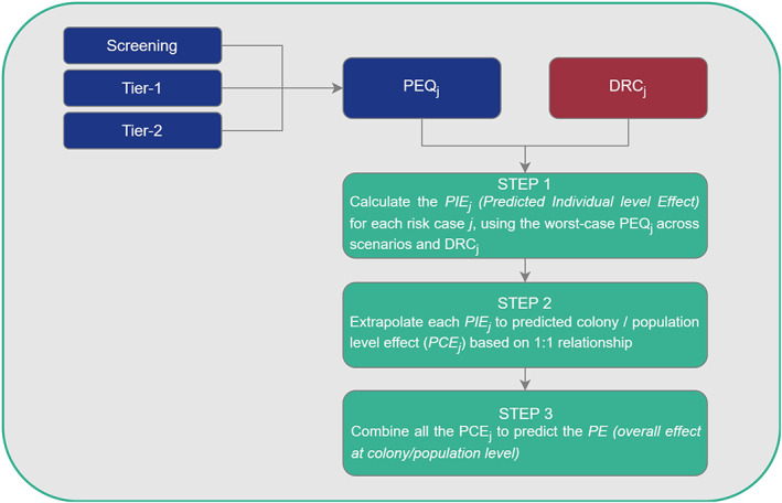
Combined risk assessment in relation to the exposure‐tier
If a substance is found to show time‐reinforced toxicity, the predicted individual level effect for the chronic dietary risk case should be calculated differently: instead of the standard 10‐day DRCj, a lifespan DRCj (covering a 27‐day lifespan) should be used, together with a PEQi calculated for a 27‐day exposure period (see also Section 8.2.1). An additional risk assessment for the winter period must be performed as well (see also Section 8.2.2).
As explained in Chapter 3, it is strongly recommended, based on the problem formulation, to start the risk assessment using the screening and Tier 1 exposure estimates. Depending on the outcome of this risk assessment, it is suggested to continue with the Tier 2 of the exposure. However, applicants could decide to address the risk identified in the Tier1 assessment directly by generating higher tier effect studies.
Screening assessment
For the screening assessment, the PEQi, calculation is performed based on simplified exposure models, as described in Section 5.6.
The predicted individual level effect (PIE) is calculated based on the screening level PEQi and the related DRCj values, for each of the risk cases (acute contact, acute dietary, chronic dietary and larvae) (see Section 7.1.1). The predicted individual level effects are then combined to determine the overall predicted effect at the colony level (see Section 7.1.3), which can be compared to the SPG. Note that if a substance presents time‐reinforced toxicity, the risk assessment should be based upon Tier 1 exposure estimates (see below), i.e. a screening level risk assessment cannot be performed because exposure estimates are calculated based on different assumptions.
If an assessment, based on the combined approach which includes a screening exposure‐Tier, indicates that the high risk cannot be excluded, a risk assessment with Tier 1 exposure estimations must be performed.
Tier 1 assessment
For Tier 1, the exposure estimation is performed based on the models described in Section 5.1. These more complex, but more realistic model assumptions result in a lower exposure estimation compared to the screening step. This exposure estimation is to be performed for all relevant exposure scenarios. The worst‐case PEQi, is selected from the exposure scenario that dominates the exposure (see also Section 4.3).
The next steps of the combined risk assessment approach are performed in the same way as for the screening level assessment.
Tier 2 assessment
If the risk assessment based on the exposure‐Tier 1 indicates that high risk cannot be excluded (i.e. SPG not met), a risk assessment based on exposure‐Tier 2 is recommended. It is noted that if the risk was not excluded at the Tier 1, the conclusion on the risk assessment is drawn based on Tier 1 unless risk refinements are available.
In the Tier 2 exposure assessment, several of the parameters in both the contact and dietary exposure models can be refined. Refer to Sections 5.4 and 5.5 for details on the options for refinement and the need to generate further data. Using the refined parameter values, refined shortcut values can be calculated, which in turn can be used in the model to calculate the Tier 2 PEQi.
If the risk assessment based on exposure‐Tier 2 still indicates that high risk cannot be excluded (i.e. SPG not met), a higher tier risk assessment has to be performed (see Chapter 3). If higher tier risk assessment is not available, the conclusion on the risk assessment is drawn based on the lower Tiers.
7.3. Implementation of the combined risk assessment approach for bumble bees and solitary bees
As mentioned in Section 1, the magnitude dimension of the SPG for bumble bees and solitary bees was discussed by risk managers on the basis on the consolidated evidence provided by EFSA (EFSA, 2022). A majority of MS risk managers agreed to select the option of ‘undefined threshold’ of acceptable effect indicated in the EFSA document (EFSA, 2022), and to more frequently require higher tier data in order to better understand the level or protection that would be appropriate for these bee groups, in the current absence of knowledge.
Based on an ‘undefined threshold’, a lower tier risk assessment scheme cannot be implemented since there are no values which would allow interpretation of any quantitative lower tier outcome.
However, in this guidance, exposure estimation and hazard definition for bumble bees and solitary bees is possible, although these are characterised by considerable uncertainty due to the lack of specific data, which may have led to very conservative estimates in some cases.
Thus, in principle the combined approach described in Section 7.1 and its implementation in the tiered approach, can be applied also for these groups of bees when a defined threshold of acceptable effects is agreed. However, it is not recommended to apply this scheme until this is defined.
For the future implementation of such an approach, applicants and risk assessors can refer to Chapters 5 and 6 for the exposure and hazard characterisation respectively, to apply step 1 as described in Section 7.1.1. Regarding the step 2 i.e. extrapolation of effect from individual to colony/population described in Section 7.1.2, the WG propose to apply the same the 1:1 relationship relative to the propagation of effects from individual to colony/population since is also considered conservative for these bee groups. The combination of the effects (step 3) as described in Section 7.1.3 would also be appropriate for calculating the overall predicted effect based on the addition of responses at the colony/population level.
8. Time‐reinforced toxicity
A substance shows time‐reinforced toxicity (TRT) when its toxic effects from exposure to low doses for a long period of time are higher compared to effects from exposure to higher doses for a short period of time (i.e. its toxic effects are reinforced by exposure time). Note that this phenomenon was called ‘accumulative toxicity’ in the EFSA (2013).
The risk assessment scheme for time‐reinforced toxicity is shown in Figure 15. This scheme can be split into two main parts: a first part which focusses on the hazard and assesses whether a substance shows time‐reinforced toxicity; a second part which is the actual risk assessment for those substances that show time‐reinforced toxicity.
Figure 15.
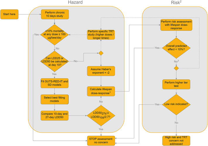
- 1: Lifespan dose–response is calculated using the selected GUTS model, for both the active period and winter scenario. 2: This part has to be duplicated for the active period and the winter (inactive) period. 3: When an effect > 10% is predicted, either higher tier studies can be performed, or a specific TRT laboratory study can be executed. This second option is only applicable when this conclusion of > 10% effect is reached on the basis of the worst‐case assumption that Haber's exponent = −2.
The risk assessment part of the scheme is only relevant for substances that were found to show time‐reinforced toxicity in the hazard part. When this is not the case, the standard Tier 1 chronic risk assessment as described in Chapter 3 is considered sufficient to address the risk from long‐term exposure. However, if a substance is identified as showing time‐reinforced toxicity, this is no longer true, and the risk assessment below supersedes the standard chronic risk assessment.
Below, each part of the overall scheme is further described. For further background on the methods and the origin of the parameter values used, please refer to Annex G of the supplementary document.
8.1. Hazard assessment
The hazard assessment part of the flowchart shown in Figure 15 is intended to answer the question of whether or not a substance shows time‐reinforced toxicity. The steps to do so are described in Section 8.1.1 below. If a substance is found to show time‐reinforced toxicity, a dose–response covering the whole lifespan has to be determined, which will later be used in the risk assessment. The TRT risk assessment methodology is described in Section 8.1.2.
8.1.1. Determining whether a substance shows time‐reinforced toxicity
The determination of whether a substance shows time‐reinforced toxicity is based on data from the standard 10‐day chronic honey bee toxicity study according to OECD test guideline 245 (OECD, 2017a). Therefore, the starting point is to collect data from the available study.
This hazard assessment is based on a methodology which relies on the use of GUTS modelling. For a short introduction to the GUTS modelling framework, please refer to Section 4.4.1 of Annex G to the supplementary document. For further details on the background for the methodology used, please refer to Section 4.4.4 and 7.1.1 of that Annex G.
Step 1: check whether an assessment is necessary
The first step is to check whether the following conditions are met in the standard 10‐day toxicity study:
-
1Was the mortality ≤ 10% at any dose ≥ 100 μg/bee per day?
-
–If yes, then a TRT assessment is not necessary.
-
–If no, go to step 2.
-
–
This possibility to waive a further assessment for time‐reinforced toxicity was included to avoid unnecessary work and potential additional testing for substances of low toxicity to bees. The rationale for selecting the threshold of ≤ 10% mortality at any dose ≥ 100 μg/bee per day is described in Annex G to the supplementary document.
Note that if the highest dose tested in the available chronic 10‐day test is below 100 μg/bee per day, step 1 of the scheme does not apply. In that case, proceed to Step 2.
Step 2: check whether a robust GUTS‐RED model can be fitted to the data
For a robust calibration of GUTS‐RED models to data from a 10‐day chronic toxicity study, a level of mortality should be reached at the end of the 10‐day test period that allows calculation of an LDD50 or LDD25 value for at least day 10. Therefore, the following conditions should be met:
-
2Can a LDD25 or LDD50 be calculated at the end of the exposure period (day 10)?
-
–If yes, fit both a GUTS‐RED‐IT and GUTS‐RED‐SD model to the data, and proceed to Step 3
-
–If no, select one of the following options:
- Perform a new 10‐day chronic toxicity study (according to OECD 245), using higher doses, and start again at step 1 using the newly obtained data
- Perform a new chronic toxicity study, with a longer duration. Fit both a GUTS‐RED‐IT and GUTS‐RED‐SD model to the data, and proceed to Step 3
- Assume the substance has TRT properties, with a worst‐case Haber's exponent of −2. Calculate the lifespan dose–response as described in Section 6.4, and proceed to the risk assessment.
-
–
When option 2a to perform a new chronic toxicity study using higher treatment doses is chosen, these doses have to be chosen so that the observed effects will increase, and at least an LDD25 can be calculated at the end of the testing period. This should enable GUTS model fitting in Step 3a. Alternatively, when in the available study the highest tested dose was below 100 μg/bee per day, a new test up to at least 100 μg/bee per day could be performed, so that this can be used in Step 1. It is acknowledged that for substances of poor solubility, this might not be technically feasible using the technical active substance. In that case, performing a 10‐day test (OECD 245) with a formulation instead of the technical active substance could be an option (as also proposed in Section 6.1.1). Alternatively, option 2b could be considered.
In option 2b, a new chronic study with a longer duration is performed. With the exception of the duration of the study, the study design should be based on OECD 245. To assess the validity of such a study, the validity criteria from OECD 245 apply, at least to the data for the first 10 days of the test. For the time period beyond 10 days, additional validity criteria for the control are not considered necessary, as control mortality inevitably will increase over time. Note that the GUTS model, which is used in Step 3, is able to discriminate between background mortality and mortality from toxicant effects. Refer to Annex G to the supplementary document for some additional recommendations for the study design.
It should be noted that in the description of Step 2b above, it is assumed that it will be possible to use the data from the study with longer duration (also called ‘life‐long’ or ‘time‐to‐effect’) test to fit a standard GUTS‐RED model. It is expected that this will be possible in most cases. However, should the treatment‐related mortality in the life‐long test still be too low to enable a GUTS model fitting, this can be considered as an indication that time‐reinforced toxicity will not be an issue for that substance.
In option 2c, it is assumed that the substance has TRT properties, with a worst‐case a Haber's exponent of −2. An explanation on why the value of −2 is a worst‐case can be found in Section 7.1.1 of Annex G to the supplementary document.
Step 3: fit both GUTS‐RED‐IT and GUTS‐RED‐IT models to the data and select the best performing model
As it cannot be known a priori whether the GUTS‐RED‐SD or GUTS‐RED‐IT model will result in a better fit to the data, it is mandatory to use both models for TRT analysis. Both models can be fitted to the data using currently available (semi‐)automated calibration and prediction tools, by which the required output for the TRT assessment can be generated. The performance of both the fitted GUTS‐RED‐SD and GUTS‐RED‐IT models is compared based on the normalised root mean square error (NRMSE) for model calibration, and the model with the lower NRMSE value is the better performing one and should be selected.
Note that in all standard GUTS implementations background mortality is described by a single parameter. While this is generally sufficient for 10‐day tests, where the control mortality must remain below 15%, it may not be the case for life‐long tests, where background mortality is not expected to be constant over time. In that case, a modified version of GUTS, which uses a 2‐parameter model for control mortality has to be used. Please refer to Section 5.1 of Annex G for a detailed explanation of this modified version to be considered.
Step 4: compare the 10‐day and 27‐day LDD50 and decide on TRT
As a final step to determine whether a substance shows time‐reinforced toxicity, the 10‐day and 27‐day LDD50 values should be derived from both the GUTS‐RED‐SD and GUTS‐RED‐IT models fitted to the data. If
| (22) |
then there is no concern about TRT. However, if this condition is not fulfilled i.e. LDD50,27d < LDD50,10d/2.7, TRT cannot be excluded.
Since it is possible that the outcome is different between GUTS‐RED‐SD and GUTS‐RED‐IT, the following decision scheme should be followed to know upon which model to base the conclusion:
-
–
If neither the GUTS‐RED‐SD nor ‐IT model indicates TRT: it can be concluded that the substance does not show TRT. No further TRT risk assessment is required;
-
–
If both the GUTS‐RED‐SD and the ‐IT model indicate TRT: it can be concluded that the substance shows TRT. Calculate the lifespan dose–response as described in Section 6.4 and proceed to the risk assessment;
-
–
If one model indicates TRT and the other does not: use the suggested metrics (NRMSE based on calibration data) to decide which of the two models to use:
-
○
If one model clearly fits better (shows lower NRMSE values), base the conclusion for TRT on the outcome from that model (i.e. compare the LDD50,10d and LDD50,27d derived from that model). Depending on the outcome, no further TRT risk assessment is required, or a lifespan dose–response as described in Section 8.1.2 needs to be calculated before proceeding to the risk assessment;
-
○
If there is no clear difference between both models, use the worst case (which will likely be the SD model). In that case, it can be concluded that the substance shows TRT. Calculate the lifespan dose–response as described in Section 8.1.2, and proceed to the risk assessment.
-
○
8.1.2. Calculating the lifespan dose–response
If following the steps described in Section 8.1.1, a substance is identified as showing time‐reinforced toxicity, or a worst‐case approach assuming a Haber's exponent of −2 is followed, a risk assessment which covers the whole lifespan of a bee should be performed (see Section 8.2). In order to be able to perform such a risk assessment, the dose–response relationship for a period of exposure that covers the whole lifespan should be known.
The WG agreed to consider two scenarios in the risk assessment: a scenario that covers the active period of the bees (i.e. summer), and an inactive winter scenario (for further details, see Section 8.2). A dose–response relationship for the whole lifespan should therefore be calculated for both scenarios, using a lifespan of 27 and 182 days for summer and winter bees, respectively.
GUTS‐RED models fitted to the chronic toxicity data can be used to determine the dose–response at any time point. If in Step 3 of the workflow described in Section 8.1.1, one of the models (either GUTS‐RED‐IT or GUTS‐RED‐SD) was identified as better matching the data, the parameterisation from the best model should be used to determine the 27‐ and 182‐day dose–response. If there is no clear difference between both models, the one resulting in worst‐case estimated 27‐ and 182‐day dose–response should be used.
If a worst‐case approach assuming a Haber's exponent of −2 is followed, the linear C vs. t relationship (on a log–log scale) is used as a basis to calculate the lifespan dose–response. Since this option will likely be used in cases where the maximum effect is small (i.e. no reliable LDD25 can be obtained from the data), a surrogate 10‐day dose–response can still be derived.
Based on previous analysis (e.g. EFSA CONTAM Panel, 2022), there are indications that the slope becomes steeper with increasing exposure durations. This empirical finding presents a rather straightforward conceptual explanation. With increasing exposure times, the LDD50 gets closer to the time‐independent No‐Effect Dose (NED). By reducing the difference between the doses causing no effect and 50% effect, the dose–response becomes steeper. In the current risk assessment scheme, a shallower slope represents a worst case, i.e. when fixing the LDD50, the effect caused by a certain dose below the LDD50 is higher for a shallower dose–response. It should be highlighted that the focus on the lower half of the dose–response (below the LDD50) is sensible, though actually an effect higher than 10% would breach the SPG.
In consideration of the above, shifting the 10‐day dose response curve to the left, without changing its shape (i.e. slope), is very likely to represent a worst‐case estimate of the lifespan dose–response. This is equivalent to assume that the linear C vs. t relationship (on a log–log scale – cfr. Equation (2) in Annex G to the supplementary document) is valid not just for the LDD50, but for any LDDx of the dose–response.
For any LDDx:
| (23) |
where t1 can be day 10, and t2 the total duration of the lifespan considered. The equation further reduces to:
| (24) |
Thus, the 10‐day curve is shifted by a factor of 7.29 and 331.24 to the left in order to get the 27‐days and the 182‐days curves, respectively.
8.2. Risk assessment based on TRT
For substances for which there is concern for time‐reinforced toxicity following the first steps of the flowchart in Figure 15, the standard chronic risk assessment (see Chapter 7 for further details) might underestimate the risk from long‐term exposure. Therefore, for such substances, a specific risk assessment, which covers the whole lifespan of a bee, should be performed. This specific risk assessment supersedes the standard chronic risk assessment.
As described in Annex G to the supplementary document, the risk assessment as described below should only be performed for honey bees for the time being.
The hazard characterisation to be used in this risk assessment is the lifespan dose–response. It was agreed to consider two scenarios in the risk assessment: one that covers the active period of the bees (i.e. a summer scenario), and one that covers the inactive/overwintering period (i.e. a winter scenario). The input parameters to calculate the exposure and the different steps of the risk assessment are discussed below for both scenarios.
8.2.1. Risk assessment for the active period
For the lifespan risk assessment during the active period, it is assumed that a honey bee will live for 27 days. This value was derived from data collected in the systematic review on bee background mortality (EFSA, 2020). Based on this data set, the median lifespan of bees during the active period is 27 days (90th perc = 41.7 days; 5th perc = 17.5 days).
Given that the standard chronic risk assessment also focuses on bees during the active period, the same method for estimating the dietary exposure can be used in the lifespan risk assessment (see Chapter 5). The values for the different parameters (e.g. RUD and DT50 in pollen and nectar, daily food consumption, etc.), as used in the standard risk assessment, can also be used here. There are only two points specific for the TRT assessment:
The time window for calculating time‐weighted average concentrations (called ‘w’). Where the standard risk assessment considers a time window of 10 days (corresponding to the duration of the standard 10‐day chronic oral toxicity study), a time window of 27 days (corresponding to the median lifespan, see above) is used in the lifespan risk assessment.
Pollen and nectar consumption. During their entire lifespan, honey bee workers undergo changes in their diet in relation to the tasks they execute. Thus, for this specific case, a combination of subsequent diets was considered. Specifically, it was assumed that bees perform nursing activities for 10 days (pollen and nectar consumption), then 8 days of additional in‐hive tasks (nectar consumption similar to the nursing phase, no pollen consumption) and 9 days of foraging activity (higher nectar consumption due to flying activities, no pollen consumption). See Section 5.3.5 for more details.
Taking into account the points above results in specific shortcut values, which are shown Appendix B of this guidance. These shortcut values are used to estimate the PEQ for the whole lifespan.
As in the standard chronic risk assessment, the predicted individual level effect is then estimated using the relevant PEQ and the lifespan dose–response. This is combined with the other risk cases to estimate the overall predicted effect at the colony level (see Chapter 7).
8.2.2. Risk assessment for winter bees
During the winter period, honey bees will not forage for fresh pollen and nectar, but will feed on the stored food in the hive (i.e. honey). Therefore, whether honey bees are exposed to the pesticide depends on the presence of residues in the honey. Taking into account that beekeeping practices in Europe are highly variable, and that there are a lot of practices which can change the exposure over winter (e.g. dividing colonies), it is not possible to give a fully realistic estimate of the extent to which bees will feed on potentially contaminated honey. Therefore, for the lower tier risk assessment, it is assumed that all food during winter consists of contaminated honey.
For the winter bee scenario, a lifespan of 6 months (=182 days) was agreed by the WG. Note that this is a very rough estimate of the winter or inactive period for bees. Please refer to Section 7.2.2 of Annex G to the supplementary document for details on how this was derived.
As stated above, it is assumed for the lower tier risk assessment that winter bee diet will consist of 100% contaminated honey. Based on this, the dietary exposure is estimated consistently with the exposure models presented in Chapter 5. Specific values for some parameters are defined irrespective of the exposure model being used. These are:
Sugar consumption from honey: in temperate regions, during winter, bees consume 8.8 mg of sugar/day to maintain the nest temperature at 5–8°C in the periphery and 15–20°C in the centre (Rortais et al., 2005);
Sugar content in honey: as in EFSA (2013b), the water content of honey is assumed to be 18%. Therefore, the sugar content of honey would then be 82%;
Dissipation rate in honey: Given that there is no data currently available on the DT50 of active substances in honey, it was agreed to use a worst‐case value for the Tier 1 risk assessment (i.e. 1,000 days), which results in no appreciable dissipation.
It should be noted that for the winter bee risk assessment, only the treated crop scenario is considered. It is acknowledged that in some cases, this might not cover for all other possible exposure scenarios. However, this is a pragmatic decision, as it was not possible to develop a winter bee assessment for the other exposure scenarios within the timeframe available to the WG. Focussing only on the treated crop implies that a winter bee risk assessment should not be performed for crops that are not attractive to bees, or that are harvested after pesticide application but before flowering. Since contamination in honey originates from nectar foraging only, a winter bee scenario is also not relevant for crops attractive for pollen only. In contrast, in line with the standard risk assessment, a winter bee risk assessment should also be performed for applications made before flowering.
8.2.2.1. Above‐soil contamination
The following equation is used to calculate the PEQ due to dietary exposure for the winter bee scenario for applications performed at BBCH stages > 10 (spray applications and granules):
| (25) |
Where: AR = Application rate (g/ha)
SV = shortcut value for dietary exposure through honey
The shortcut values are calculated using the following equation:
| (26) |
Where: 8.8 mg/day is the consumption of sugar in winter
= 0.82 is the sugar content of honey.
PCUDho = Predicted concentration per unit dose in honey (mg/kg)
= , with k = ln(2)/DT50 and w = 182 days.
A database for RUD values in honey was compiled based on data from residue trials in honey, available for eight substance (33 individual data points) (see Annex G to the supplementary document). Based on this data set, a 90th percentile RUD for residues in honey of 3.0 mg/kg was derived. For granular applications at BBCH > 10, this RUD is used as a surrogate, together with a dust formation factor of 0.1 and a safety factor of 3, consistent with the strategy applied for this application method in the derivation of the Ef described in Section 5.3.2.
It should be noted that in the other parts of the risk assessment, the SVs used for calculating the exposure are determined using a Monte Carlo simulation (see Section 5.3.4 for details). This takes into account the range and distribution of the values of the different parameters to derive an overall 90th percentile SV value. However, for the winter bee scenario, there is only one parameter (RUD) for which a range and distribution is available. Therefore, using the 90th percentile value for the RUD would give a similar result for the SV as when a Monte Carlo simulation is performed. Given that the former is easier, the SVs for Tier 1 for the winter bee scenario are obtained via a simple calculation according to the equation above, and by using the 90th percentile RUD value for honey (3.0 mg/kg). Using the values for the other parameters as mentioned above, this results in the following SVs, shown in Table 30.
Table 30.
Shortcut values for winter bees (above soil contamination)
| Application | Shortcut value (μg/bee per day) |
|---|---|
| Spray applications | 0.03 |
| Granules | 0.009 |
8.2.2.2. Through‐soil contamination
Consistent with what was agreed for the above‐soil contamination model, the 90th percentile value from the database for RUD values in honey (3.0 mg/kg, see Appendix B to this Annex) is considered for through‐soil contamination as well. As presented in Section 5.1.2.1, residues in nectar for contamination via soil can be estimated by using PECpw. The same is considered to be true for residues in honey. Thus, the following equation is used to calculate the PEQ due to dietary exposure for the winter bee scenario for applications performed at BBCH stages < 10 (seed treatment, spray applications and granules):
| (27) |
Where: = Predicted Environmental Concentration in pore water (mg/L = mg/kg)
8.8 mg/day is the consumption of sugar in winter.
= 0.82 is the sugar content of honey.
k = ln(2)/DT50 and w = 182 days.
In the Tier 1 of the exposure assessment, consistent with what is reported in Section 5.3.14, the PECpw is assumed to be 1 mg/kg for any application regime where the cumulative application rate is not higher than 4.5 kg/ha. In cases where the cumulative application rate is higher than 4.5 kg/ha, a Tier 2 exposure estimation must be conducted that requires a GAP specific PECpw calculation, as described in Section 5.5.14.
Note that all parameters used for Tier 1 exposure estimations are in this case fixed, therefore, the exposure estimation for winter scenario and through‐soil contamination model is 0.010 μg/bee per day.
As in the standard chronic risk assessment, the predicted individual level effect is then estimated using the relevant PEQ and the lifespan dose–response. For the winter scenario, only continuous dietary exposure through honey consumption is considered. In addition, there are no larvae during winter. Therefore, the other risk cases (i.e. adult acute contact and dietary, larvae) are not relevant in this case. The winter scenario is thus a stand‐alone assessment. The predicted individual effect level will correspond to the overall predicted effects at the colony level.
8.2.3. Refinement options
If the Tier 1 risk assessment for the active period and/or the winter bee scenario shows that high risk cannot be excluded (i.e. the SPG is breached), as next step, it is possible to refine the exposure estimation according to the exposure‐tier and/or to perform a specific TRT study, as also described in Section 8.1.1. The latter would especially be useful for those substances for which initially no LDD50 or LDD25 could be calculated from the available 10‐day study (and hence no GUTS‐RED models could be fitted), and therefore, a Haber's exponent of −2 was assumed for calculating the lifespan dose–response.
For the lifespan risk assessment for the active period, the exposure is estimated using the same dietary exposure method and parameters as in the standard risk assessment, with only minor differences (see Section 7.2.1). Therefore, all possible refinement options that can be used in the standard risk assessment can also be used here (see Sections 5.4 and 5.5).
For the lifespan risk assessment for the winter bees, the only two parameters in the dietary exposure model that could be refined using substance‐specific data are the residues in honey and the DT50 in honey. When the through‐soil model is applicable, a possible refinement of the residue level entails a better characterisation of the PECpw at the time of flowering, as explained in Section 5.5.14.
Data on the residues in honey could be obtained from available studies in the residue section of a pesticide dossier (e.g. submitted for setting an MRL in honey). However, experience with sampling honey for the bee risk assessment is relatively scarce, as during the active period, honey is not considered a good estimator of exposure (see Annex B of the guidance document). During winter, some of the issues that honey presents during the active period (i.e. different levels of maturation, concentrations and re‐dilution) should be less relevant.
For both RUD and dissipation studies, it is important that samples combine different spots from different combs, in order to be representative of the whole storage. For dissipation studies, this strategy would also minimise the risk that samples are only representative for material (i.e. nectar) collected by the bees during a specific moment of the active period. Should this be the case, this would be a confounding factor for determining the dissipation kinetics.
For dissipation studies, it is also important to make sure that the active substance of concern is present in the capped honey cells in sufficient concentrations at the start of winter. Otherwise a suitable kinetic decline cannot be determined.
More specific guidance on the sampling strategy cannot be given for the time being. It is expected that further recommendations could be provided when more experience is gained.
The lifespan of a winter bee of 182 days is a very rough and conservative estimate. In theory, this value could be refined if more detailed data became available. However, it should be noted that any refinement of the winter bee lifespan would have only a rather minor effect on the estimated lifespan dose–response (refer to Annex G to the supplementary document for details). Therefore, this kind of (general) refinement is not considered very useful, unless the outcome of the risk assessment is borderline or it can be demonstrated that the length of the winter period is substantially less than 3 months, which is rarely the case in Europe.
8.2.4. Higher tier risk assessment
When a low risk could not be demonstrated in lower tier, the final step is to conduct higher tier effect field studies. The requirements for such studies are described in detail in Chapter 10. Generally, these requirements are the same for substances that show time‐reinforced toxicity and those substances that do not. However, if a substance shows time‐reinforced toxicity (regardless of whether the risk assessment for the active period or the winter bee scenario fails at lower tier), a field study should be sufficiently long to ensure that potential effects following long‐term exposure are addressed. In practice, this means that the study should not be started later than September and last until next spring, thus including overwintering and observing the honey bees for at least half a year.
When risk refinements are not available, the conclusion will be drawn based on the outcome of the lower tiers.
8.3. Active substance vs. formulation
Time‐reinforced toxicity is an intrinsic property of an active substance. Therefore, the TRT assessment as described in the sections above should always be performed for active substances.
In some cases, however, a chronic toxicity study with the formulated plant protection product (PPP) is also required (see Section 6.1.1 of the guidance document). This will be the case if, based on acute data, the PPP was found to be more toxic compared to the active substance, or when the PPP contains multiple active substances.
Overall, whenever chronic data with the PPP is available, these data should be used in the hazard assessment for TRT (See Section 6.4). If the outcome based on the PPP data is different compared to that based on the active substance data, the worst case should be considered further.
In case of multiple active substances in a PPP, the TRT assessment should be performed for all actives. If 2 (or more) active substances show TRT, a lifespan risk assessment considering all these substances should be performed, using mixture toxicity. If only one active substance shows TRT, the lifespan risk assessment is only to be done for this single substance.
9. Sublethal effects on honey bees in risk assessment
9.1. Overall strategy
The SPG for honey bees focusses on colony strength and while the relationship between direct mortality and colony strength is relatively straightforward to establish (Section 1.3) there is no way to link observed sublethal effects and colony strength. Despite this, concern for sublethal effects on wild and managed bee populations has been growing, primarily as a response to the broad range of harmful sublethal effects that have been reported across many bee species (see Annex K of the supplementary document). Due to the growing concerns and specific calls for greater inclusion of sublethal effects to protect bee populations, the WG has decided to review the current provisions for assessing sublethal effects in the new guidance document.
Some major barriers to developing a comprehensive assessment of sublethal effects are their almost limitless diversity, the lack of standardisation of measurement and lack of a proven link to the SPG. To address these issues, the WG has decided to focus primarily on a subset of sublethal effects, in particular those that very obviously alter bee behaviour. The rationale for this is that large scale behavioural changes may interfere with important tasks, such as foraging, which would be expected to have a strong mechanistic link/relationship to colony strength. For example, a persistent sublethal effect that reduces the ability of honey bee workers to forage would reduce the amount of food available to a colony and the number of individuals in the hive which would eventually result in fewer bees and a smaller colony size that may eventually breach the SPG. Additionally, the WG believes that behavioural observations can be readily incorporated into standard laboratory tests, allowing applicants to identify potential concern for adverse effects on foraging behaviour. If a potential concern is raised, this can be further investigated in specific assays.
The WG have provided recommendations for a number of lower and higher tier tests; however, the pinnacle of the risk assessment process is still the field test. Ultimately, the goal of the risk assessment for bees is to show whether the SPG is met (see Chapter 3) and fully reliable and complete higher tier tests can directly demonstrate compliance with the SPG. Thus, at higher tiers if the SPG is met then even if sublethal effects occur they do not impair the colony strength sufficiently to be considered a concern. Therefore, if a reliable and complete higher tier risk assessment is available (see Chapter 3), there is no need to specifically consider sublethal effects and an assessment does not need to be carried out. In all other cases, a sublethal assessment focussed on effects on foraging behaviour of honey bees is required. It is noted that sublethal effects are assessed in parallel to the risk assessment based on mortality data, but in case field studies are available these will cover sublethal effects.
As internationally agreed test guidelines are mostly limited to honey bees (with the exception of acute toxicity testing for Bombus spp.), the WG agreed to limit the assessment for sublethal effects to honey bees for the time being. In the meantime, valuable experience can be gained with this new approach.
The strategy is shown in Figure 16 and explained below. Details on the assessment strategy are given in the supplementary document Chapter 9.
Figure 16.
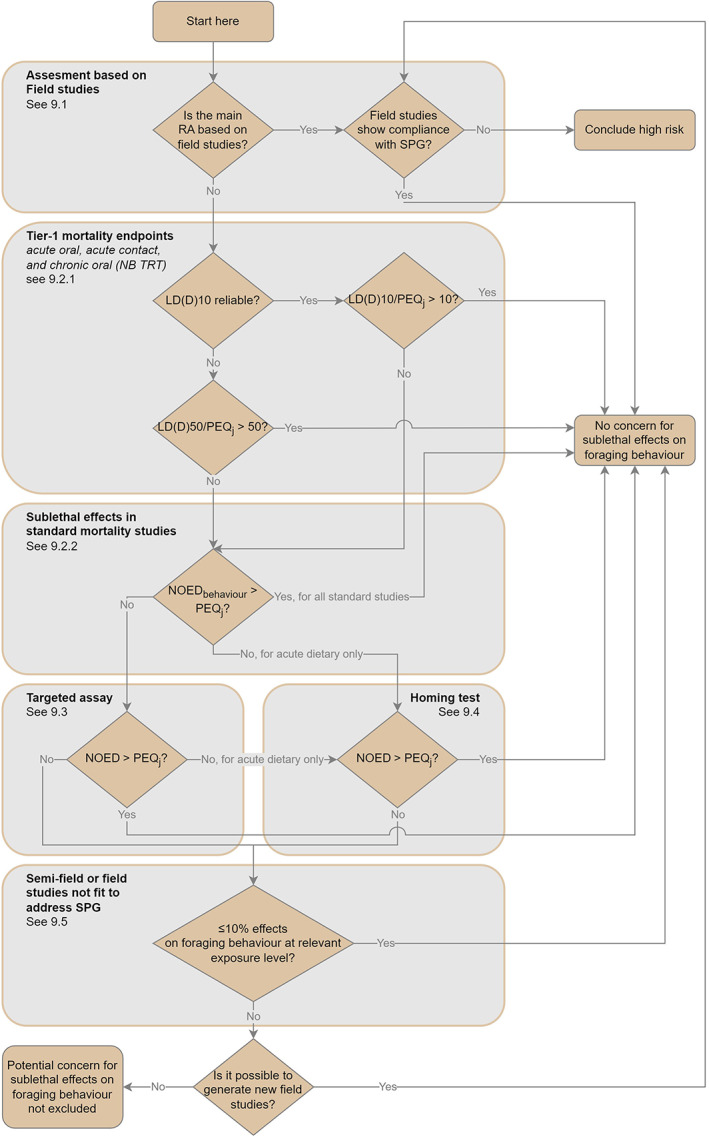
Assessment strategy for sublethal effects
As our understanding of honey bee colony dynamics evolves it may be possible to use modelling to investigate the link between sublethal effects on foraging behaviour and colony strength, but this is currently not possible. Therefore, the WG acknowledges that in cases where a risk for sublethal effects on foraging behaviour is identified, the impact on colony strength is still unknown. The outcome of the sublethal risk assessment described here can therefore only be ‘concern for sublethal effects indicated’ or ‘no concern for sublethal effects indicated’.
9.2. Strategy for triggering concern from lower tier information on honey bees
9.2.1. Toxicity/exposure ratio using mortality endpoints
The first step in the sublethal assessment is to estimate a ‘no concern level’, i.e. a sufficiently low exposure (i.e. PEQj) which is not expected to affect foraging behaviour of exposed bees. The ‘no concern level’ can be calculated as the LD(D)10 divided by 10. If a reliable LD(D)10 cannot be calculated, the LD(D)50 divided by 50 can be used, which provides a more conservative no concern level.
The no concern level should be calculated separately for the acute contact, the acute dietary and the chronic dietary dose–response information and compared separately to the corresponding PEQj.
In step 1, a concern from sublethal effects in the lower tier is triggered by a PEQj which exceeds the no concern level calculated either by:
1a) Where a reliable L(D)D10 exists: a PEQ j that is greater than the LD(D)10/10, i.e. L(D)D10/PEQ j > 10;
1b) Where a reliable L(D)D10 does not exist: a PEQ j that is greater than the LD(D)50/50, i.e. L(D)D50/PEQ j > 50
PEQj values are calculated according to Chapter 5. The most refined PEQj available, i.e. from the highest exposure assessment tier, can be used;
For limit tests with (virtually) no mortality, the following stands: LD(D)50 = LD(D)10 = NOED, meaning that case 1a) is applicable;
If a substance/product shows time‐reinforced toxicity (TRT), the risk assessment should consider the full lifespan. Since foraging behaviour is only relevant for summer bees, the 27‐d LD(D)50 and corresponding PEQj should be used (see Chapter 5 for more information).
If the PEQj is lower than the ‘no concern level’ (1a, 1b) for each of the three standard studies on honey bees, i.e. acute contact, acute dietary and chronic dietary, then no concern for adverse effect for foraging behaviour can be concluded and no further consideration is needed. If the PEQj is higher than the ‘no concern level’ a potential concern is identified and the risk assessor should proceed to the next step (step 2 in Section 9.2.2).
9.2.2. Using pattern of sublethal effects seen in the laboratory tests
In the second step, the ‘no‐concern level’ is calculated from the proportion of abnormal behaviours observed during the standard laboratory tests on honey bees (acute dietary, acute contact and chronic dietary) and the amount of food consumed by the bees. The WG propose using the regular observations required in OECD Test Guidelines 213, 214 and 245 (OECD, 1998a, b, 2017a) to determine if exposure to a PPP influences the behaviour of bees in laboratory experiments. Further standardisation can be achieved by following the recommendations in the supplementary materials of Tosi and Nieh (2019). As changes in behaviour in laboratory studies cannot be directly linked to the SPG, any statistically significant difference between the behaviour of the treatment and control groups should be treated as indicative of a potentially important sublethal effect that requires further investigation.
Given the historical focus on mortality in both risk assessment guidance and lower tier testing (EFSA, 2013; OECD, 1998a,b) there has been a lack of guidance and standardisation for the recording of behaviour. Therefore it is possible that behavioural data from older studies may be less reliable than mortality data. In older studies where abnormal behaviour is frequently recorded it is likely that any behavioural effects were sufficiently obvious to record easily. However, in studies with no or very few abnormalities, i.e. where no difference between the control and any tested dose, it is impossible to differentiate between experiments where the PPP elicited no abnormal behavioural or those where the observations were insufficient to detect them. Therefore, before using studies with very few instances of abnormal behaviour the risk assessors must evaluate whether the behavioural data are reliable.
This decision can be made by considering the age of the study and/or the level of detail in the description of the behavioural observations in the methods section. For example, studies which generated data prior to the publication of OECD (2017a,b,c), which provided an initial description of the abnormal behaviours that should be recorded (forming the basis of the assessment in this guidance document), may be considered less reliable. However, these studies may be considered reliable if they provide a description of both the observational methods and a description of the categories of behavioural endpoints that are recorded, and these are consistent with those recommended in OECD 245. Also, it may be considered whether the observations are in line with other studies and information on the tested compound.
Sections 9.2.2.1–9.2.2.3 of the guidance document explain how to derive a NOEDbehaviour from the standard laboratory tests.
2) If the NOED behaviour from the standard studies is higher than the PEQ j , there is no concern indicated from sublethal effects on foraging behaviour.
If this is not the case, additional studies are needed, see step 3 in Section 9.3 and step 4 in Section 9.4.
9.2.2.1. Statistical analysis of behavioural effects to derive ‘no concern level’ (NOEDbehaviour )
Ideally, the appropriate statistical model should be able to describe not only the dose–response trend which is the focus of this analysis, but also the temporal pattern of abnormal observations. This may be problematic, however, as individuals showing behavioural abnormalities may revert to showing normal behaviour as time goes on, potentially resulting in no clear, consistent trend over time (unlike for mortality studies where the trend is, by definition, increasing). Accounting for the temporal pattern may thus hinder the analysis and produce results which are difficult to interpret. As a result, the WG recommends analysing the data aggregated across the experimental period. A single aggregate proportion should be calculated for each cage (the sum of daily observations of abnormal behaviour divided by the sum of the daily count of live bees). The analysis should then focus on investigating whether the aggregate proportions show an increasing trend with dose levels.
The WG recommends following the OECD (2006) recommendation to use a test for trend combined with a ‘step‐down’ procedure. This test is focussed on the detection of a monotonic (increasing) trend and should be appropriately selected among the range of options presented in OECD (2006). A good choice, to provide an example, could be the Rao‐Scott adjusted Cochran‐Armitage test (RSCA) (Rao and Scott, 1992), which has several desirable advantages: It is generally the most robust choice for quantal data (proportions), it allows for overdispersion and it takes experimental replication into account (Green et al., 2018).
An appropriate test for trend is chosen and the data is analysed using a step‐down procedure following the method described in OECD (2006), meaning:
The test for trend should be performed for data from all the treatment groups including the control. The cages should be incorporated as subgroups (or clusters) in the test;
If the test is significant (α = 0.05) then there is an increasing response across all dose levels. The high dose group is omitted and the test for trend is repeated with the remaining dose groups;
The procedure is continued until the test is non‐significant – there is no increasing response across the remaining dose groups. The highest concentration remaining at this stage is the NOEC.
9.2.2.2. Statistical analysis of behavioural effects to derive the ‘no concern level’ for food consumption (NOEDbehaviour ,food)
In acute and chronic dietary studies, it should also be tested if the PPP induces changes in food consumption. The statistical analysis should be based on an ANOVA and include a dose, day and day by dose interaction in order to be able to compare the mean volume of food consumed between each treatment group and the control (Rao and Scott, 1992; Green et al., 2018). The comparison should be done for each day; a Bonferroni–Holm adjustment for multiple comparisons can be used (OECD, 2006).
9.2.2.3. Worked example of how to analyse the behavioural observations after exposure to a PPP
The aim of this example is to demonstrate the calculation of a NOEC from data taken from an anonymised dossier study. The data consists of a 10‐day chronic exposure study where the number of abnormal behaviours, as described in OECD (2017a,b,c), were recorded every 24 h. The data is presented in Figure 17 and was analysed using a RSCA test with a step‐down procedure, as described in Section 9.2.2.1. The model returned significant p‐values for the first four steps (all p < 0.001) indicating that each of the four highest concentrations of the PPP had a higher proportion of abnormal behavioural observations than the control. When the model included only the control and the lowest tested concentration of the PPP, 156.25 mg a.s./kg, the trend was not significant (p = 0.483), indicating that this can be considered as the NOEC value from this experiment. In the 156.25 mg a.s./kg treatment group, the accumulated mean uptake of the test item was 43.99 μg a.s./bee/d. Thus, the interpretation of this test would be that a PEQdi,ch of < 4.399 μg a.s./bee/d would not trigger a concern for sublethal behaviour, a PEQdi,ch ≥ 4.399 μg a.s./bee/d would trigger a concern for sublethal effects and the applicant should proceed to larger scale experiment behavioural laboratory experiments or higher tier tests.
Figure 17.
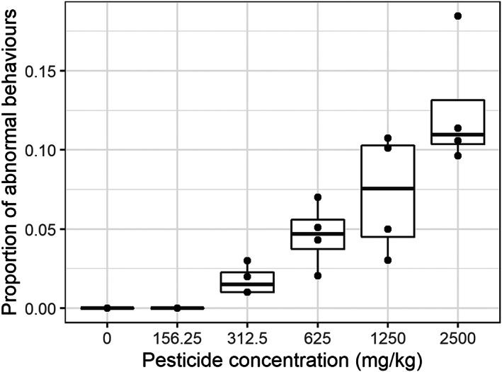
Boxplot showing the proportion of abnormal behaviour across a range of PPP concentrations aggregated across the entire experiment, note that the y axis is truncated at 0.2
9.3. Specific behavioural assays on honey bees
If a potential concern is raised based on the standard laboratory studies, targeted behavioural assays can be done. These studies should have similar study designs and statistical methods as the mortality tests but may use lower doses to include the ‘no concern level’. However, it has to be ensured that the predicted exposure of the exposure assessment tiers for the proposed GAP are covered in the test. In addition, the following modifications to improve the quality of the data collection sublethal effects should be implemented:
Even with training, interpreting the behaviour of an animal can be subjective. In order to minimise any unconscious bias it is required that any behavioural results are generated blind (i.e. the observer does not know which treatment has been given to which group);
The minimum number of replicates should be increased. The applicant has to demonstrate that the experiment is large enough to detect an effect size of at least 10% more observations of abnormal behaviour in the treatment group relative to the control group with an alpha of 0.05 and a power of 0.8;
Further standardisation of behavioural assessments can be achieved with the recommendations in the supplementary materials of Tosi and Nieh (2019).
In addition, the WG notes that using the OECD test designs, behavioural observations can only be monitored as the proportion of individuals behaving abnormally at any point, making the unit of replication the cage. If individual bees can be marked, either by using paints or identification tags, then the behaviour of each individual can be recorded at each time point, potentially making the unit of replication the individual and increasing the statistical power of the test to detect an effect. This is however considered a potential future improvement, not implementable at present.
The modifications mentioned above (blind observer and increased number of replicates) can also be implemented directly in the mortality tests. The WG urges consideration of these in future modifications of the OECD guidelines for acute and chronic adult bee toxicity tests. The NOEDbehaviour from the targeted assay should be compared to the relevant exposure level. This step supersedes the outcome of the previous steps.
3) If the NOED behaviour from the modified assays is higher than the PEQ j of the exposure assessment tiers, there is no concern indicated from sublethal effects on foraging behaviour.
9.4. Homing flight study
The homing flight study is not required under the current data requirements, but an OECD guidance document has been published (OECD, 2021). The homing flight study can only be used as a refinement of a concern indicated from acute dietary exposure (either in step 2 or 3). The dose level in the test needs to cover the acute daily intake of a forager bee.
4) If the NOED homing test is higher than the PEQ ac,di , there is no concern from acute sublethal effects on foraging behaviour.
9.5. Higher tier endpoints
If a fully reliable and complete higher tier risk assessment for honey bees shows compliance with the specific protection goal, apparently, even if sublethal effects occurred, they were not of such importance that colony strength was impaired. However, a situation can be envisaged in which the available higher tier studies are not fully reliable to study effects on colony strength (e.g. they are too short or measure inadequate or incomplete endpoints) but can still be used to study other effects. In such a case, assessment of effects on foraging behaviour in semi‐field or field studies can be useful and informative for the overall risk assessment. It is important to minimise variability between hives (e.g. with regard to number of adult bees, brood and food stores) to reduce the change of detecting an effect where there is none. Guidance for equalisation of colonies is given in Annex C to the guidance document.
In most cases a sublethal effect on foraging behaviour will not be equivalent to the death of an individual bee, however, in the worst cases, e.g. moribund bees, a bee that is still alive will be removed from the workforce and will be functionally dead from the perspective of the colony. Therefore, as a realistic worst‐case assumption, any sublethal effects will be assumed to be equivalent to death. The value of 10% is chosen to match the SPG. If the difference in sublethal effects between treatment and control is ≤ 10% it is assumed that, even in the worst cases, the reduction in colony size will be unlikely to breach the SPG. If the difference is > 10%, the link to colony strength is less clear. In the absence of data, the possibility that the sublethal effect will reduce the colony size sufficiently to breach the SPG cannot be excluded.
Therefore, and in the absence of a set protection goal for sublethal effects, it is conservatively assumed that any reduction in foraging behaviour of > 10% causes an effect of > 10% on colony strength. Thus, > 10% effect is chosen as trigger. In future, modelling (e.g. with ApisRAM) (Duan et al., 2022) may be useful to investigate the link between these effects and colony size.
An adverse effect on foraging behaviour is defined here as a > 10% reduction (compared to the untreated control) of one or more of the following endpoints:
The amount of pollen collected per flight (in mass)
Ideally the amount of pollen is measured in higher tier studies. However, it can also be estimated by proxy through the number of bees returning with pollen (see below). In future, the amount of pollen may be estimated through the size of the pollen pellet on the incoming bee as determined by analysis of video images. Current methods allow the number of bees returning with pollen in a set period to be counted (see below) and for the mass of pollen to be recorded using pollen traps. By combining these methods, the amount of pollen collected per flight can be estimated. For pollen traps, use the recommendations of Human et al. (2013) and Delaplane et al. (2013). However, it is noted that it may be challenging to measure the number of bees returning with pollen during the full period that the pollen trap is active.
The number of bees returning with pollen
This is considered as proxy for the amount of pollen entering the hive. It can be measured by visual observation of the hive entrance, by a human or automated observer.
For human observers, the recommendations of Delaplane et al. (2013) should be followed:
To control for between‐colony variation due to time of the day, the investigator should: (1) limit observations to days and time of day with good flight conditions; (2) randomise the numeric order in which colonies are measured; (3) measure all colonies within a relatively narrow window of time; and (4) limit colony observations to the same time window over successive days;
Two observers sit to the side of a colony, each positioned well enough to the side to avoid obstructing the flight of the bees. Each observer has a hand‐held counting device and one keeps time;
For one 15 min counting episode, each observer counts and records count foragers returning with, and without, corbicular pollen loads in order to derive proportion of foragers collecting pollen. Note that the length of the counting episode per hive may need to be adapted to reach a sufficient power of the study;
-
The mean of the two observers is derived and the data reported as total number of foragers returning and the proportion of foragers collecting pollen.
The observations should be done at the same time for paired control and treated fields.
Technology for automated observation is already available and will be further developed in the coming years. The WG was not in a position to give detailed guidance on the use of this technology; nevertheless, the WG considered some of those example as promising tools for these observations. Therefore, it is expected that such tools will supersede the human observers method in the near future. The accuracy of any such tool used in the risk assessment must be proven.
The duration of a foraging flight (in minutes/flight)
This parameter is considered useful if the homing test indicates a concern. The two parameters listed above (on pollen collection) also cover concern from the homing test, so if one of these is available, assessment of foraging flight duration is not obligatory.
The duration of a foraging flight can be assessed when individual foragers are marked. In order to assess a sufficient number of individuals, RFID (radio‐frequency identification) technology is likely required. Useful guidance for RFID is provided in the OECD guidance document on the homing flight test (OECD, 2021). Recommendations are also given in Scheiner et al. (2013). If deviating from OECD (2021), the particular methods chosen should be justified.
These endpoints can be measured in higher tier studies, either semi‐field or field. The number of bees returning with pollen (or, if feasible, the amount of pollen collected per bee flight) should always be assessed, and the duration of a foraging flight is only obligatory if the homing test indicates a concern.
To measure the endpoints, the observations should be carried out at least 2 days prior to treatment (to demonstrate that the bees are acclimatised), and then as close to the application as possible (1–2 h before) and at several intervals after treatment (OEPP/EPPO, 2010). Observation timing will depend on the specific situation but should include the days at which exposure in the higher tier effect study is expected to be highest. For a spray treatment, this is likely the day of application and the following 3 days. Observations should cover both the hours directly after application and the most active foraging hours of the day. For seed treatments and other pre‐flowering applications, since the peak of exposure is likely unknown a priori, the whole flowering period should be covered by frequent observations, at least at every second day during the flowering period. As a general rule, the days and time of the day with good flight conditions should be selected for these observations. Effect calculations should be presented and evaluated per day.
The statistical analysis should be conducted according to the general approach for higher tier studies (see Annex C of the guidance document and Chapter 10.1). The applicant should apply a one‐sided equivalence test () for each endpoint, with an equivalence limit corresponding to a 10% reduction in the treated test compared to the control, to prove that there are no adverse effects on foraging behaviour. Based on the current data it is not possible to provide indications on the number of replicates required to reach an adequate statistical power of the test.
Two additional endpoints were considered but not included as requirement. The density of foragers on the crop (bees/m2) was considered informative in the past for showing that exposure took place in a test. However, for the purpose of the sublethal assessment it is not considered useful, since the data are usually scarce and it is difficult to statistically compare controls with treatments. The amount of nectar collected (μL/flight) is considered a useful endpoint but it is not currently included due to the technical challenges measuring nectar uptake in bees.
In conclusion, step 5 of the assessment strategy is:
5) The foraging behaviour endpoints have to be investigated in higher tier studies at an exposure level that corresponds to the proposed GAP and should be sufficiently high, i.e. it should represent at least a 90th percentile exposure as predicted by one of the exposure assessment tiers. For more details, see Chapter 10. If no effect > 10% was seen at this exposure level, there is no concern from sublethal effects on foraging behaviour.
If a concern is still indicated after this step, the only possible refinement is field studies that directly study colony size and show compliance with the SPG (see Section 9.1 above).
10. Higher tier risk assessment
10.1. Introduction
In the higher tier of the risk assessment, the effects on bees are studied under more realistic conditions. For honey bees, the scope of the higher tier is to evaluate the risk of a PPP under realistic use conditions when a high risk was not excluded at the lower tier, and to check if the agreed SPG is met. For bumble bees and solitary bees, a majority of MS risk managers agreed to select the option of an ‘undefined threshold’ of acceptable effects, which was given as an option in EFSA (2022). Until the SPGs for bumble bees and solitary bees are defined, a majority of MSs agreed to require higher tier studies more frequently, allowing a better understanding and protection of these bee groups. In the current absence of knowledge, therefore, higher tier tests should generally be produced.
This guidance document considers three types of higher tier effect studies: field, semi‐field and colony feeder studies. Colony feeder study can only be performed with for eusocial bees that form colonies. Below we provide a brief description of the aims, methodology, main considerations, and the endpoints for each study type. These studies follow internationally agreed and widely used guidelines, e.g. EPPO 170/2010, as far as possible. Detailed guidance is given in Annex C.
The aim of higher tier effect studies is to measure the magnitude of effects on the study endpoint(s) after a field realistic worst‐case exposure to the PPP use under evaluation. Since the relevant endpoints under field realistic exposure conditions can be best studied in field conditions, the most suitable option is conducting a field study. However, under specific circumstances (see section below and Figure 4 in Chapter 3), the other study types, which are less complex, could be considered. In all cases, the outcome of certain measurements (i.e. endpoints) from the exposed group(s) is compared with control group(s). All conditions of the exposed and control groups should be sufficiently similar with the only important difference being the PPP treatment itself.
The statistical analysis is based on the test of equivalence. This marks a substantial departure from the most common approach followed for effect studies. Indeed, the equivalence approach, is based on the assumption that the PPP causes adverse effects, since risk was not excluded at lower tier. In a standard approach, the starting hypothesis is that the PPP has no effect – that there is no risk. In the standard approach, evidence can only indicate – with a pre‐established level of confidence ‐ the presence of an effect of an undefined magnitude. When this is not the case, the starting hypothesis is not disproven, and the results are often interpreted as a complete lack of effects and thus as a ‘proof of safety’. However, such a conclusion is not supported with the same level of confidence. In fact, the level of confidence for such conclusion can hardly be set a priori, and even the evaluation a‐posteriori presents challenges and pitfalls. A test of equivalence reverses the points of view, placing the burden of proof on the ‘safer’ hypothesis. The starting assumption is that the effect is larger than the SPG – that there is a high risk. The experimental evidence is used to prove the opposite, that the effect (if any) is smaller than the SPG – that the risk is low. If there is not enough evidence, the final conclusion is that the risk is high, which is considered an appropriately conservative outcome. As a direct consequence, there is no need for risk assessors to recommend minimum levels of replications or sample size in the study. Equivalence testing allows the higher tier to actually statistically override the high risk conclusion of the lower tiers, rather than simply failing to prove it. The statistical methods are described in Section 2 of Annex C. Further details on the statistical requirements are included in the detailed description of each study type included in the same annex.
10.2. Higher tier studies for honey bees
10.2.1. Honey bee field study
Circumstances when the study type is useful
This study type is recommended when the lower tier risk assessment indicates no clear dominance of a particular exposure route or risk case and the predicted reduction in colony size (i.e. predicted effect greater than the SPG) is indicated to arise from (1) a combination of different routes of exposure, (2) a combination of effects on adults and larvae, (3) or solely a dietary risk to adults.
Methodology to be followed
Colonies with free flying bees are studied in field conditions at sites in different agricultural landscapes. The test colonies are located at the edge of the treated or the control fields. In order to confirm sufficient exposure, residues entering the hive have to be measured (see Sections 10.5 and 10.7.8). The endpoint(s) must be studied for all colonies in the same way.
Endpoint to be studied
The mandatory endpoint to be studied, and that is the subject of the statistical comparison, is the colony size, characterised by the number of adult bees in a colony.
Further definitions and detailed descriptions of the requirements are included in Sections 4.1 and 4.2 of Annex C.
10.2.2. Honey bee semi‐field study
Circumstances when the study type is useful
A) This study type is recommended when the lower tier risk assessment indicates that the predicted reduction in colony size greater than SPG is dominated by the risk arising from contact exposure.
B) This study type is recommended when, in the lower tier risk assessment, a concern for sublethal effects was flagged.
Methodology to be followed
Bee colonies enclosed in large cages are studied. The cages are in field conditions and include a flowering crop, which is either treated with the test PPP or treated with water (control) and treated with a substance toxic to bees (positive control). In order to prove sufficient exposure (see also Sections 10.5 and 10.7.8), the foraging activity has to be observed. The endpoint(s) must be studied for all colonies in the same way.
Endpoint to be studied
A) The mandatory endpoint that should be studied, and which is the subject of a statistical assessment, is forager mortality.
B) The endpoint to be studied, and which is the subject of a statistical assessment, is foraging behaviour.
Further definitions and detailed descriptions of the requirements are included in Section 4.1 and 4.3 of Annex C.
10.2.3. Honey bee colony feeder study
Circumstances when the study type is useful
The study type is recommended when the lower tier risk assessment indicates that the predicted effects on colony size reduction greater than SPG is clearly dominated by the risk arising from effects on larvae.
Methodology to be followed
Free‐flying bee colonies are studied in field conditions, but in a location with limited food resources. The test colonies are fed with sugar solution and/or pollen spiked with the test PPP or with sugar solution and/or pollen without the PPP (control) and treated with a substance toxic to bees (positive control). The exposure is controlled by the concentration(s) of the offered solution (see also Sections 10.5 and 10.7.8). The endpoint(s) (see below) must be studied for all colonies in the same way.
Endpoint to be studied
The mandatory endpoint that should be studied, and which is the subject of the statistical comparison, is the number of covered brood cells.
Further definitions and detailed descriptions of the requirements are included in Sections 4.1 and 4.4 of Annex C.
10.3. Higher tier studies for bumble bees
Field studies and semi‐field studies with bumble bees aim at investigating similar endpoints as mentioned in Section 10.2 for honey bees, but are performed under somewhat different conditions. The field test is the most realistic assessment of a PPP. Nevertheless, depending on the problem formulation and the PPP under evaluation, a semi‐field test might be conducted.
10.3.1. Bumble bee field study
The aim of these studies is to gain insight into the risks for bumble bee colonies under realistic field conditions while still maintaining sufficient control over the experimental conditions (e.g. Rundlöf et al., 2015; Woodcock et al., 2017; Ruddle et al., 2018). As field tests, these higher tier tests represent the best available experimental method to evaluate potential effects of the use of PPPs in the field.
Methodology to be followed
Colonies with free‐flying bees are studied in field conditions at sites in different agricultural landscapes. The test colonies are located at the edge of the treated or the control fields. In order to prove sufficient exposure, residues entering the hive must be measured (see Section 10.5, below). The endpoint(s) must be studied for all colonies in the same way.
Endpoint to be studied
The mandatory endpoints which should be reported and analysed will be 1) the colony weight over time (weeks 0–8), which represents the colony strength, and 2) the number of queen‐sized cocoons (eclosed + intact) present in the final census, which represents the colony reproductive output.
Further definitions and detailed descriptions of the requirements are included in Chapter 5 of Annex C.
10.3.2. Bumble bee semi‐field study
The purpose of this test is to measure the effect of a PPP use on the bumble bee colony under semi‐field conditions. This test combines multiple realistic elements, including the requirement for bees to actively forage on a treated crop (e.g. Tamburini et al., 2021; Wintermantel et al., 2022); however, it is not fully realistic, and as such the results of this test may be superseded by the results of a field test.
Methodology to be followed
Bee colonies enclosed in large cages are studied. The cages are in field conditions and include a flowering crop, which is either treated with the test PPP or treated with water (control) and treated with a substance toxic to bees (positive control). In order to prove sufficient exposure, flight activity has to be observed (see also Section 10.5, below). The endpoint(s) must be studied for all colonies in the same way.
Endpoint to be studied
The mandatory endpoints which should be reported and analysed will be colony weight over time (weeks 0–8) which represents the colony strength and the number of produced queen‐sized cocoons (eclosed + intact) present in the final census which represents the colony reproductive output.
Further definitions and detailed descriptions of the requirements are included in Chapter 5 of Annex C.
10.3.3. Bumble bee colony feeder study
The purpose of this test is to measure the effect of a PPP on the colony using exposure to pesticides delivered in food in combination with more realistic environmental conditions in the field. The test is based on studies, where a colony is provided with dosed food inside the colony box rather from foraging on treated crops (e.g. Whitehorn et al., 2012; Gill et al., 2012; Botías et al., 2021; Arce et al., 2017; Siviter et al., 2018). This test requires the least resources of the three tests and may be favoured by applicants; however, as the exposure route is the least realistic of the higher tier tests, the results of this test may be superseded by semi‐field or field tests.
Methodology to be followed
Free‐flying bee colonies are studied in field conditions. The test colonies are fed with sugar solution spiked with the test PPP or with sugar solution without the PPP (control) and treated with a substance toxic to bees (positive control). The exposure is controlled by the concentration(s) of the offered solution (see also Section 10.5, below). The endpoint(s) (see below) must be studied for all colonies in the same way.
Endpoint to be studied
The mandatory endpoints which should be reported and analysed will be the colony weight over time (weeks 0–8), which represents the colony strength and the number of produced queen‐sized cocoons (eclosed + intact) present in the final census, which represents the colony reproductive output.
Further definitions and detailed descriptions of the requirements are included in Chapter 5 of Annex C of this guidance document.
10.4. Higher tier studies for solitary bees
Field studies and semi‐field studies with solitary bees also aim at investigating endpoints important for understanding effects on the population, but include a number of parameters which differ from those of honey or bumble bee (semi‐)field studies. The field test is the most realistic assessment of a PPP. Nevertheless, depending on the problem formulation and the PPP under evaluation, a semi‐field test might be conducted.
It is also noted that the test species for which guidance can be provided, based on the current available knowledge, is O. bicornis, but O. cornuta or other solitary bee species could be considered. Further considerations to address the uncertainties around the extrapolation of the results to the numerous EU solitary bee species are strongly encouraged.
10.4.1. Solitary bee field study
The aim of these studies is to gain insight into the risks for solitary bee populations under realistic field conditions while still maintaining sufficient control over the experimental conditions (e.g. Rundlöf et al., 2015, Woodcock et al., 2017, Ruddle et al., 2018). As field tests, these higher tier tests represent the best available experimental method to evaluate potential effects of the use of PPPs in the field.
Methodology to be followed
Free‐flying bees at nesting units (bee populations) are studied in field conditions at sites in different agricultural landscapes. The test bees are located at the edge of the treated or control fields. To prove sufficient exposure, residues entering the nest must be measured (see Section 10.5, below). The endpoints (see below) must be studied for all populations in the same way. The primarily test species for which guidance is provided is O. bicornis, but O. cornuta or other solitary bee species could be considered.
Endpoint to be studied
The recommended endpoints that should be studied, and which are the subject of the statistical comparison are:
Nesting activity as the proportion of nesting females in relation to the emerged number of females in the starting population;
- Reproduction in the form of:
-
○Number of brood cells;
-
○Number of cocoons;
-
○Number of emerged females and males in the next generation;
-
○
Population growth rate as the multiplicative product of nesting activity, number of offspring and proportion daughters.
It should be noted that the recommended endpoints above are relevant for Osmia spp. In case other test species are used, the endpoints might need to be adapted to the biology/ecology of the test species; nevertheless they should be related to the next generation population size.
Further definitions and detailed descriptions of the requirements are included in Chapter 6 of Annex C.
10.4.2. Solitary bee semi‐field study
The purpose of this test is to measure the effect of a PPP use on the solitary bee population under semi‐field conditions. The test is based on enclosing a population and providing exposure through plants (e.g. Stuligross and Williams, 2020; Franke et al., 2021). This test combines multiple realistic elements, including the requirement for bees to actively forage on a treated crop, however, it is not fully realistic, and as such the results of this test may be superseded by the results of a field test.
Methodology to be followed
Bees (bee populations) enclosed in large cages are studied. The cages are in field conditions and include a flowering crop, which is either treated with the test PPP, treated with water (negative control) and treated with a substance toxic to bees (positive control). To evidence sufficient exposure, the flight activity must be observed (see also Section 10.5, below). The endpoints (see below) must be studied for all populations in the same way. The primarily test species for which guidance is provided is O. bicornis, but O. cornuta or other solitary bee species could be considered.
Endpoint to be studied
The recommended endpoints that should be studied, and which is the subject of the statistical comparison are:
Nesting activity as the proportion of nesting females in relation to the emerged number of females in the starting population;
- Reproduction in the form of:
-
○Number of brood cells;
-
○Number of cocoons;
-
○Number of emerged females and males in the next generation;
-
○
Population growth rate as the multiplicative product of nesting activity, number of offspring and proportion daughters.
It should be noted that the recommended endpoints above are relevant for Osmia spp. In case other test species are used, the endpoints might need to be adapted to the biology/ecology of the test species; nevertheless they should be related to the next generation population size.
Further definitions and detailed descriptions of the requirements are included in Chapter 6 of Annex C.
10.5. Exposure in higher tier effect studies vs. ExAG
As explained above, higher tier studies, depending on the study type and on the organisms tested, provide a range of effect endpoints. In such studies, effects need to be investigated at an exposure level in line with the ExAG, i.e. 90th percentile worst‐case exposure for the compound under evaluation. Therefore, appropriate exposure regimes and levels must be ensured in the higher tier studies. To compare the exposure levels with the PEQj, it is recommended to calculate the Estimated Exposure Dose, defined as EEDj in Chapter 3, which has to be expressed in the same unit as the PEQj. This means that, in addition to the biological observations, it is necessary to consistently verify the exposure levels, e.g. via measurement of residues in pollen and nectar, and use these measurements to estimate the EEDj in the specific study. Details on how to estimate the EEDj are included in Annex C. The EEDj is compared with the related PEQj in order to assess t if levels of exposure in higher tier studies were adequate and therefore if observed effects (or lack of effects) can be linked to the ExAG. This is further explained in Section 10.7.8. The comparison should be carried out with PEQj based on independent measured residue trials (e.g. Tier 2) (see Chapter 5 and Annex B), but if not available, the PEQj from lower tier exposure assessment should be used. This is illustrated in Figure 18.
Figure 18.
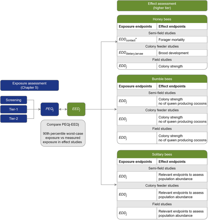
Exposure regime in higher tier effect studies should be estimated and compared with the PEQ in order to assess the plausibility of the biological observations in the studies. The suffix ‘j’ indicates the 4 risk cases (acute contact, acute, dietary, chronic, larvae). *The EEDcontact in semi‐field studies, does not require to be estimated since the exposure level in the study is confirmed by the flight activity as described in Annex C of this guidance document
It is noted that a specific estimation of the EED is not necessary for semi‐field studies, since the foraging activity (number of honey bees foraging in the crop) or the flight activity at the colony/nest entrance (the total number of bumble bees or solitary bees flying in and out) is considered to be a sufficient proxy. These observations are used in order to show that the bees are actively foraging on the crop and are therefore exposed to the PPP. In this case the EED corresponds to the full amount of PPP applied in the study, which should be in line with the GAP under evaluation.
In colony feeder studies, the EED should be estimated based on the food consumption during the study.
When the effect endpoint is colony strength the EED should be estimated for all the relevant risk cases and compared to the related PEQ.
10.6. Ecological models for the support of higher tier risk assessment
10.6.1. General suitability, requirements and possible advantage of ecological models for higher tier regulatory risk assessment
Ecological models for chemical risk assessment simulate essential processes in ecological systems, and how these processes are affected by chemicals. These models can improve the mechanistic understanding of the risk of PPPs and make uncertainties in the risk assessment explicit and are therefore explicitly recognised by the WG as important tools for higher tier pollinator risk assessment.
Pollinator colony or population models can be very useful tools to support and generalise the interpretation of ecotoxicological studies such as (semi‐)field tests. In higher tier pollinator risk assessment, they could in particular be used to extrapolate exposure observations from field tests to other locations or field situations, including other uses than tested in a (semi‐)field test, to analyse the influence of additional stressors on the risk of the PPP, or to analyse the potential effectiveness of risk mitigation measures.
Ecological models for the higher tier refinement of pollinator risk assessment, however, as any other modelling tool used in regulatory risk assessment, have to prove their suitability, more precisely, they need to show appropriateness for supporting the regulatory question and their respective performance before they can be considered for regulatory risk assessment. One critical issue is whether an ecological model provides an appropriate model complexity, meaning that the model needs to be sufficiently complex to match the relevant real‐world processes and traits of pollinators in a landscape context. For a honey bee colony model, this could mean that internal processes in a beehive such as egg laying, brood care, recruitment, pollen and nectar inflow and consumption, are considered as simulated processes, with external influences, such as food quality and quantity, the performance of individual bees, the impact of varroa mites and infectious diseases and other possible stressors, each accounted for in an appropriate level of detail. Additional processes linked to the interaction of the colony with the surrounding environment (e.g. foraging in the landscape) are generally extremely important aspects that determine an appropriate level of complexity. That does not mean that all processes need to be simulated based on first principles, since simulation models are, and need to be, a simplification of reality. The key issue by definition must be the potential simulation model's ability to cover these influencing factors in an appropriate way.
More specifically, if the model is used to simulate exposure to a PPP and resulting effects, processes underlying these aspects should also be demonstrated to be considered appropriately. This includes for example the fate of the substance in the environment and within the hive, mechanisms that cause the exposure of the bees, the quantification of such exposure, and the link between the simulated exposure and the simulated effects. In this case, it is appropriate to refer to these models as ecological effect models. In fact, the aforementioned appropriateness can and must be demonstrated by comparison between model results and observed data, for example, from a relevant semi‐field or field experiment. Based on a thorough definition of the corresponding environmental scenario, colony model predictions should show a good overlap with the dynamics of real observations, ideally with no or little calibration of model parameters, and should demonstrate matching with the most important patterns. For complex models, such as honey bee colony models, the demonstration of appropriateness can in general be performed on two levels. First, on the level of the general model, which means that parts and modules of the model can be shown to match with general experimental observations, e.g. the age structure of a honey bee colony matches with common observations. Second, the colony model needs to demonstrate that it can predict observations from a specific field trial within reasonable limits of prediction quality, and under consideration of the usually high uncertainty and variability of observations in the field.
Closely related to this second level of a check of appropriateness is the need to define respective environmental scenarios. For modelling bee population dynamics, the landscape context, i.e. type, amount and location of nectar and pollen resources, and weather conditions such as temperature, rain and sunlight/irradiation are crucial input for the model, and need to be defined in the form of environmental scenarios. When using ecological models for extrapolation, additional environmental scenarios can be defined, e.g. to allow simulations of bee populations under less favourable conditions, e.g. in a low‐resource landscape, or for other landscape composition or under different weather conditions. It is required that ecological models demonstrate reasonable simulations results for such a variety of environmental scenarios which can represent the different landscapes across Europe.
Depending on the intended use, in addition to the above‐described need for an evaluation of the appropriateness of the model for describing a specific (set of) field experiment(s) will likely require additional work on scenario definition. If the aim of the application of the ecological model was for example to extrapolate to other areas of use (see below), carefully underpinned scenarios need to be selected that represent either the entire variety of environmental conditions for the intended area of use of the compound (from which a desired percentile of probability of occurrence could be selected), or ‘realistic worst case’ environmental conditions in order to protect a bee population under worse‐than‐average conditions, but for e.g. 90% of all situations.
For the possible acceptance for use in regulatory risk assessment appropriate, comprehensive and transparent documentation of an ecological model is an important precondition. The use of an established protocol/format standard for the documentation of individual‐ or equation‐based models such as ODD (Overview, Design concepts and Details) or TRACE (TRAnsparent and Comprehensive model Evaluation) is here considered as an important requirement. The documentation should allow and support the critical evaluation of the ecological modelling approach and the corresponding scenarios. A general framework how to evaluate ecological and ecotoxicological models for regulatory risk assessment of PPP was outlined in the EFSA scientific opinion on Good Modelling Practice (EFSA PPR Panel, 2014), but further relevant and appropriate documents might be used for that purpose in the future.
After listing many demands and challenges, and under the very clear requirement of using (semi‐)field data for testing model performance in the beginning of any higher tier ecological modelling study, the WG would like to underline the value and reason to perform ecological modelling in higher tiers. The WG agreed on that, if an ecological model has been generally assessed positive for a use in regulatory risk assessment, and has been proven to perform well against specific (semi‐)field data, it can be trusted to deliver useful and relevant results for the risk assessment. Ecological models might then be used to calculate margins of safety for the simulated scenarios. Those simulated margins of safety can then support decisions in higher tier risk assessment, for example via being used as line of evidence. Especially if simulated margins of safety are large, unclear decisions on the acceptance of field studies could be taken with higher certainty.
10.6.2. Examples of supportive use of ecological (effect) models
Currently, there is no honey bee, bumble bee or solitary bee model established for immediate use in regulatory risk assessment, including simulations of the exposure and effects to pesticides after spraying in agricultural fields. Therefore, the examples given below of the supportive use of ecological models in regulatory risk assessment should be considered as incomplete and illustrative for the time being. These examples refer mainly to honeybee and bumble bee colonies, and population models for Osmia bicornis. The use of models to support extrapolation to non‐standard solitary or bumble bee species is seen as highly valuable development, but the current state of such extrapolation was not seen by the WG on a level that would allow incorporation of such concepts into regulatory risk assessment.
As mentioned in Chapter 3, the WG does recommend the use of ecological models as higher tier refinement method only with the support of semi‐field or/and field data. The reason is that there are still many unknowns regarding the possible interactions between a pesticide application and its possible effects in a field situation while the models can only predict effect mechanisms which are appropriately considered and implemented. It is therefore a requirement that any higher tier assessment is checked against experimental data for the compound under assessment under realistic (semi‐)field conditions, which serves as basis to evaluate the model performance. After that testing, modelling can act as a method to aid the interpretation of the experimental data and to extrapolate those to other situations.
10.6.2.1. Extrapolation to untested conditions
One possible way to utilise ecological models was extrapolating exposure observations from field tests to other locations or field situations. In a first step, an ecological effect model would simulate exposure as observed in an exposure field study with the aim to corroborate the results. In a second step, the model could be used to extrapolate then the exposure situation to other landscapes and under different conditions e.g. weather, application times, landscape composition or other factors with the aim of refining bee colony/population exposure. In such case, it would be crucial to consider that a change in the environmental scenario should not only influence exposure, but may also alter colony dynamics and performance due to different conditions, e.g. a different food availability in the landscape, different weather, etc.
A special case concerning exposure refinement is the possible use of a simple foraging model for the calculation of exposure in a landscape context, which is proposed as a Tier 2 method (ref. Section 5.5.7 Landscape factor (LF)). While in general the same suitability criteria apply for such a model application, the model's purpose would be to simulate nectar (or pollen) foraging, not colony/population dynamics, so it is not immediately necessary to include complex colony/population‐level or ecotoxicological simulations in such foraging models. Nevertheless, such a Tier‐2 model would need to demonstrate its performance concerning nectar and pollen foraging against observations from field trials.
10.6.2.2. Effectiveness of risk mitigation measures
In a more general sense, higher tier ecological models for bees could be used to test the effectiveness of suggested risk mitigation measures (RMMs) for different ecological and agricultural practice scenarios, and to help to prioritise them. For example, the effectiveness of flower strips and the influence of their size (i.e. length/width) on the exposure of honey bee foragers in mass‐flowering crops could be simulated. This has, in a proof‐of‐concept study, already been shown (Baveco et al., 2016), and more complex higher tier modelling studies could assess the effectiveness of RMMs in similar ways.
10.6.2.3. Influence of additional stressors
One of the most crucial questions when assessing the risks of pesticide applications to bee colonies/populations in field conditions, is whether bee colonies/populations are exposed and impacted by other stressors such as limited quantity and quality of nectar or pollen in monoculture landscapes, infectious diseases, climate change, etc. These other stressors might reduce the bees' resilience and lead to more severe impacts as compared to laboratory tests or in‐field trials where some or several of these stressors can be excluded/controlled. In this case, ecological models can support higher tier experimental studies aiming at more holistic and realistic risk assessments including the consideration of multiple stressors at the landscape level. The honey bee colony model ApisRAM version 1 (Duan et al., 2022), currently under refinement by EFSA MUST‐B working group, has the potential to of support future risk assessment of PPPs in interaction with other stressors occurring at the landscape level (EFSA Scientific Committee, 2021). The model is not yet ready for use and will require robust calibration and testing before it can be used for the regulatory risk assessment of PPP, at least not before version 3 is implemented for the risk assessment of single PPP product and use (see ApisRAM implementation timeline (EFSA, online)12).
10.7. Weight of evidence and uncertainty analysis
In this guidance document a structured weight of evidence (WoE) approach is recommended for evaluating the outcome of the effect higher tier studies and use them for higher tier risk assessment.
The following section is largely based on the recommendations included in the EFSA guidance on the use of the weight of evidence approach in scientific assessments (EFSA Scientific Committee, 2017). While not aiming at being highly prescriptive, some additional guidance is provided to make the generic principles of EFSA Scientific Committee (2017) more specific to the pesticide risk assessment to bees.
10.7.1. Definitions and structure of the WoE
The building blocks of the weight of evidence process are generally referred to as ‘lines of evidence’. EFSA Scientific Committee (2017) defines the line of evidence as ‘a set of evidence of similar type’. In the context of the bee risk assessment, a line of evidence should group the whole set of homogeneous endpoints measured in all available experiments. Higher tier studies may include purely experimental studies as well as modelling simulations, which may be considered ‘in‐silico experiments’. Within this section, the generic term ‘experiments’ is used without any distinction between these typologies (EFSA, 2018a).
A single result for an endpoint measured in one experiment is operatively defined as ‘piece of evidence’, consistent with the definition reported in EFSA Scientific Committee (2017). A line of evidence may consist of a single piece of evidence, of multiple pieces of evidence from the same experiment, or of multiple endpoints from several experiments. Thus, if the building blocks of the WoE are lines of evidence, the building blocks of each line of evidence are pieces of evidence (see Figure 19).
Figure 19.
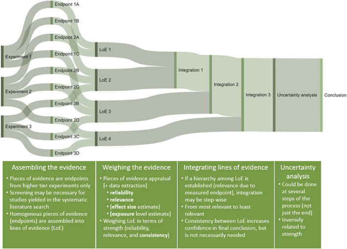
Summary of the WoE + uncertainty analysis process
As for any scientific assessment, the WoE assessment should address a specific problem formulation, which may be translated into one or more assessment questions. This step in the present document is already described in Chapter 4 and must include considerations about the uses under assessment, the physical–chemical characteristics of the active substance and potential interactions with other components of the product which may alter the environmental behaviour of the substance. However, the reader should be mindful that the problem formulation when assessing higher tier information may differ from the one formulated at the very beginning of the assessment i.e. at the lower tiers. This is because some aspects/questions of the risk assessment may already be addressed in the lower tiers, while newer ones may – under specific circumstances – arise.
EFSA Scientific Committee (2017) considers that any WoE comprises three basic steps (see Figure 19):
Assembling the evidence;
Weighing the evidence;
Integrating the evidence.
A further, separate step of uncertainty analysis (see Figure 19) is also needed to take account of any other uncertainties affecting the overall assessment.
10.7.2. Assembling the evidence
The first parts of this step, i.e. identifying and selecting evidence to include in the WoE assessment, is relatively straightforward in the context of the pesticide authorisation. The domain of the WoE is limited to the evidence submitted in the dossier, whether these are studies carried out by the Applicant or deemed relevant from the mandatory systematic review of the open literature. This also includes studies from the open literature which were flagged as relevant during the peer‐review process. The definition of specific screening/eligibility criteria for the literature review should follow the recommendations of EFSA (2011).
Within the present guidance, it is recommended to include in the WoE uniquely evidence from higher tier studies (see Section 10.2). Evidence from lower and higher tier studies is generally not comparable, thus, any integration in common lines of evidence is discouraged. In principle, evidence from lower tier studies can be used for building additional lines of evidence. Nevertheless, tiered risk assessment schemes present by definition a clear hierarchy, where results from higher tiers generally override results from lower tiers. Thus, it is expected that including evidence with low weight would not provide great benefit, when compared to the cost of integrating very heterogenous evidence. Other kinds of information related to the specific uses under assessment, the physical–chemical characteristics of the active substance, and potential interactions with other components of the product, are better used to define the problem formulation (see Section 10.6.1) rather than being used as complementary lines of evidence. However, if for any reason this is not possible, it may be considered to include this information in the evaluation of the uncertainties (Section 10.7.5).
When assembling the evidence, one critical aspect is the grouping of pieces of evidence in lines of evidence. In some cases, this is relatively straightforward. However, care should be taken when similar but not exactly equal endpoints are measured and reported. For example, some experiments may report brood‐related endpoints as ‘area of the comb covered in brood’, while other may report indexes related to brood development and termination. It is a responsibility of the risk assessor, depending on the type of WoE adopted (see Section 10.7.3) to judge whether pieces of evidence are sufficiently homogenous to be grouped in a single line of evidence.
10.7.3. Weighing the evidence
At this step of the WoE, risk assessors should evaluate the reliability, the relevance and the consistency of pieces and/or lines of evidence.
Reliability, often referred to as ‘internal validity’, reflects the internal bias, i.e. potential errors in the conduct of an experiment that results in a conclusion which is different from the truth. The method for measuring an endpoint not being reliable/accurate is an example of source of internal bias. In some instances, reliability also includes considerations related to the precision in the measurements, which relates to the sample size/level of replication in comparison with the expected variability (e.g. power of the experimental design). However, in other cases, this is assessed separately (EFSA, 2020; EFSA PPR Panel, 2022a,b). Either way, this aspect should be considered.
Relevance, also referred to as external validity, reflect external bias, which affects the extent to which the study results are generalisable to the assessment question at hand. Relevance, in the present context, may be determined by two main aspects: (1) the ability of the measured endpoint to address the assessment question, which is further considered in the part describing the integration of the lines of evidence below; (2) the representativeness of the experimental settings, which may include considerations about environmental conditions, landscape structure, nature of the tested item (e.g. formulation type), treated crop(s), application technique and regime, etc. Relevance may or may not include considerations about the level of the exposure measured/estimated in the experiment in comparison with the exposure assessment goal (see more on this in Section 10.7.8).
When performing the appraisal of the individual pieces of evidence, it is good practice to extract the relevant information in a structured manner. This may include considerations about relevance and reliability in the form of critical appraisal tool, but it may also include information on: (1) the effect size observed in the experiment for the specific endpoint (see Section 10.7.7), (2) the exposure level and duration measured/predicted/imposed in the experiment (see Section 10.7.8).
Consistency reflects the level of coherence in the available evidence. While the assessment of reliability and relevance is applicable to single pieces of evidence as well as lines of evidence, consistency can only be appraised within (at this stage of the process) and between (at the next stage of the process) lines of evidence.
Pieces of evidence appraisal
In practical terms, this phase of the WoE starts with an evaluation of the relevance and the reliability of the available evidence. While it is acknowledged that some aspects of the evaluation will be applicable to all endpoints measured in the same experiment, other may substantially differ. Thus, it is strongly recommended that such an appraisal is performed at the level of the single endpoint measured in the experiment.
At this stage, it is worth distinguishing between the two main aspects identified above that contribute to relevance. In a line of evidence grouping homogenous endpoints, the ability of the measured endpoint to address the assessment question is a constant ‐ and may in fact be determined a priori (see for example EFSA (2018b,c,d)). On the contrary, the representativeness of the experimental settings will likely differ between experiments, and thus should be evaluated carefully at this stage.
Weighing lines of evidence
Once the single pieces of evidence are appraised, the outcome can be used to appraise the strength of each line of evidence. Strength can be viewed as the degree to which the line of evidence allows achieving a conclusion for the assessment question. Overall reliability, relevance and consistency, all contribute to the strength of the line of evidence (EFSA PPR Panel, 2022a,b).
A line of evidence composed of unreliable pieces of evidence cannot be strong, even if the relevance is high and the results are consistent across experiments – it will only provide weak evidence for the conclusion, possibly associated with large uncertainties (see Section 10.6.5). Similarly, a line of evidence composed of reliable and relevant pieces of evidence, which nonetheless provide an inconsistent picture in terms of results, will generally be considered inconclusive.
One of the issues which is often debated is whether pieces of evidence classified as ‘unreliable’ should be included in the later stages of WoE. While there is little doubt that this evidence should have little to no weight in the assessment, it is here suggested that all pieces of evidence are included in the reporting, also in the phases after the appraisal: this will increase the transparency of the process and allow estimation of the impact that a different classification would have triggered as a part of the uncertainty analysis (see Section 10.6.5).
The relevance of the measured endpoint for addressing the assessment question plays a pivotal role in weighing the relative importance of the different lines of evidence. In fact, it may be appropriate in some case to establish an a priori hierarchy among lines of evidence, depending on to what degree the measured endpoints are informative for the assessment question (EFSA, 2018b,c,d). Note that this relative importance depends once again on the assessment question defined in the problem formulation and refined based upon the outcome of the lower tier risk assessment(s). For example, if a concern in the lower tier risk assessment is mainly identified for acute contact toxicity, the assessment question should mirror this. In such case a line of evidence summarising results for forager mortality is certainly more important that of any brood assessment. This ranking is, however, completely reversed if the main concern identified in the lower tiers of the risk assessment is about brood development.
10.7.4. Integrating the evidence
If a hierarchy among lines of evidence is established, the integration may be performed in a step‐wise manner, i.e. from the most relevant to the least relevant. If the most relevant line of evidence provides a conclusive answer to the assessment question with enough certainty, integration with other lines of evidence may not even be necessary. For example, if measurements of the attribute mentioned in the SPG (e.g. colony strength) provides a clear conclusive picture, no further assessment is necessary.
In many cases however, such a straightforward answer will not be available, and thus, more lines of evidence will have to be considered. The way lines of evidence are integrated depends to a large extent on the chosen methods for performing the WoE. This section is purposefully not prescriptive in this sense, and the assessor has the freedom to choose the method which is considered more appropriate for the specific case (see Section 10.6.3).
Nevertheless, as a general rule of thumb, having a consistent indication of concern or lack of it from several lines of evidence increases the confidence in the final conclusion. Thus, to some extent, the assessor should try to check the consistency across lines of evidence as well.
10.7.5. Uncertainty analysis
WoE assessment and uncertainty are closely related: the strength of any line of evidence and of the final conclusion are inversely proportional to the degree of uncertainty associated with it.
When performing an uncertainty analysis, the assessor should be mindful that, together with the uncertainty ‘intrinsic’ to the evidence, there may be additional uncertainty arising from the very same process used in weighing the evidence.
It is recommended that an uncertainty analysis is always performed together with any WoE assessment. This can be done in different ways, and uncertainty can in fact be considered at different steps of the process. Ideally, considerations about uncertainty should already be included when assessing reliability and relevance of the individual lines of evidence. However, it is even more important to clearly report the uncertainty associated with each line of evidence (See for example EFSA PPR Panel (2022a,b)). Uncertainty can also be evaluated at the very end of the assessment process, just before reaching a conclusion (see for example EFSA (2018b,c,d).
Uncertainty can be expressed in a purely qualitative manner, but attempts to quantify it to the maximum possible extent are encouraged. Reporting that makes use of structured elements (e.g. tables) generally helps the reader in getting a better overview and is thus recommended.
10.7.6. Types of WoE
EFSA Scientific Committee (2017) classifies methodologies used for WoE in four broad categories, based on where they stand in a scale from fully qualitative to fully quantitative, which to some extent also reflects a gradient in how formal the applied method is. These are: ‘best professional judgment’, ‘causal criteria’, ‘rating’ and ‘quantification’.
The present guidance purposefully avoids being too prescriptive in the methods to be followed for the WoE, as different methods may be more appropriate in different cases. However, as a general rule of thumb, it is strongly encouraged that the whole process is formalised to the maximum extent possible from the beginning of the assessment, in order to increase transparency and reproducibility. At the very least, some formality is strongly recommended in the procedure used for appraising the individual pieces of evidence, in weighing the lines of evidence and in presenting the available information in a structured way (e.g. tables and plots are preferred to long text descriptions). Establishing a priori methods for integrating lines of evidence (other than ranking them by relevance of the measured endpoint) is generally less straightforward.
Different methods may also be applied to different steps of the same WoE. EFSA PPR Panel (2022a,b) are examples of WoE integrating aspects of the category ‘rating’ (for the evidence appraisal), ‘quantification’ (for determining consistency within and between lines of evidence) and ‘best professional judgment’ (for integrating the lines of evidence, assessing uncertainty and reaching a conclusion).
10.7.7. Determining effect sizes
Irrespective of the method chosen for assessing and integrating the lines of evidence, whether this is more quantitative or qualitative (see Section 10.6.6), it is important that an effort is made to determine the magnitude of the effect observed for each measured endpoint in each available experiment i.e. each piece of evidence. In principle, both the magnitude and the temporal scale of the effect should be considered. However, for bees, the temporal scale of the effect is irrelevant in the SPG as currently defined (see Section 1.3).
‘Effects’ imply, by definition, a causality between exposure and an observed alteration of the measured endpoint, when compared to an untreated control. In reality, proving (or disproving) causality is always a complex task. As a starting point, it is recommended that deviations in both directions, i.e. favourable as well as adverse, are recorded and considered. This helps in discriminating random variability from ‘true’ effects. Similarly, it is recommended that in a WoE approach, the assessor should not rely entirely on the outcome of statistical tests. Consistency in the results from several experiments with limited power may override inconclusive statistical evaluations performed on each single piece of evidence.
Most endpoints measured in bee higher tier testing present a remarkable temporal – and in some instances spatial – variability. This complicates the determination of the effect size. A possibility is to extract and report effect sizes in terms of ranges, rather than single estimates. However, the assessor should try to focus on the most relevant time in the experiment in consideration of the characteristics of the tested substance and on the expected exposure for the uses under investigation. A knockdown insecticide with short half‐life applied to a flowering crop is expected to exert its effects soon after the application. On the contrary, effects on the number of adult solitary bees from the use of a persistent insect growth regulator may be seen only in the next generation, thus in some cases (e.g. univoltine solitary bee species) 1 year after the treatment.
10.7.8. Exposure considerations
Exposure is a critical part of the risk assessment; EFSA Scientific Committee (2017) suggests that the exposure estimates to be used in the risk assessment could be also included in a WoE as separate lines of evidence, later to be integrated with effect‐related lines. In the context of the present bee risk assessment however, this practice is not supported. This is because a procedure is already in place for estimating ‐ with a suitable level of confidence ‐ the PEQ, i.e. level of exposure in line with the exposure assessment goal (ExAG). This level should be used as a reference in assessing higher tier studies (see Section 10.5).
However, exposure in the higher tier individual experiments must be considered in the WoE. This may be done in two different ways. Exposure levels (magnitude as well as duration) can be considered in the relevance part of the appraisal of individual lines of evidence. If this approach is selected, the more the exposure level deviates from the PEQ and from the expected duration, the less relevant the resulting piece of evidence will be. The downside of this approach is that both high exposure and low exposure are considered less relevant, but without an explicit consideration of the influence played by the level of exposure on the measured endpoint. This issue could be addressed by using the second approach, i.e. considering exposure as a covariate within each line of evidence. If exposure levels influence the observed effect size in a sort of dose–response relationship, it may be possible to use this information to estimate the effect size at the PEQ. If a quantitative approach is selected, this can be performed following the principles of the meta‐regression (Thompson and Higgins, 2002). Adopting such approach may also help in addressing the ‘consistency’ aspect within each line of evidence, e.g. by explaining difference in the measured effect sizes between experiments.
11. Metabolites
Regulation (EC) No 1107/2009 requires that potentially harmful effects of an active substance and its metabolites on the environment shall be examined. According to the Regulation (EC) No 283/2013 information shall be generated to provide a basis for an assessment of the impact of the active substance and its metabolites on non‐target species, where they are of toxicological or environmental significance. Bees (honey bees, bumble bees and solitary bees) can be exposed to metabolites that are formed in pollen and nectar; the impact can result from single, prolonged or repeated exposure.
11.1. Method
The risk assessment scheme proposed in this Chapter focuses on exposure to residues following consumption of pollen and nectar that are contaminated by PPPs (dietary exposure).
A risk assessment for metabolites is triggered when:
residues of metabolites are found at or above 10% TRR (Total Radioactive Residue) and 0.01 mg eq/kg (OECD, 2007) in residue studies in pollen and nectar or metabolism studies in primary and rotation crops; OR
residues of metabolites are found at or above 10% TRR (Total Radioactive Residue) or 0.01 mg eq/kg in residue studies in pollen and nectar or metabolism studies in primary and rotation crops, and their parent (active) substance is of acute toxicity to bees (i.e. LD50 < 0.01 μg a.s./bee).
The trigger for the relevance of the metabolites was determined considering the OECD test guidelines on metabolism in crops (OECD TG 501, 2007) and metabolism in rotational crops (OECD TG 502, 2007). Apart from the concentration trigger (i.e. 10% TRR and/or 0.01 mg eq/kg), a toxicity trigger (i.e. LD50 < 0.01 μg a.s./bee) has been added to take into account possible toxic metabolites. The toxicity trigger (LD50 < 0.01 μg a.s./bee) was chosen pragmatically based on the succeeding crop scenario.
The first step is to assess whether a risk assessment is triggered for any identified metabolite in the available studies (e.g. plant metabolism studies). An overview of residue data, including recommendations on how the data should be assessed in order to obtain the relevant information on metabolites, is reported in Appendix C to the guidance document. Guidance on how to conduct the risk assessment is given in Section 11.2.
11.2. Risk assessment for metabolites
When a metabolite requires further assessment based on residue data (i.e. ≥ 10% TRR and/or 0.01 mg eq/kg depending on the acute toxicity of the parent to bees), relevant information on the hazard and exposure of the metabolite to bees has to be provided.
11.2.1. Hazard characterisation
The data requirements for metabolites are the same as for the active substance (according to the Regulation (EC) 283/2013). Therefore, the following data are required for all relevant metabolites:
Acute oral toxicity to bees;
Chronic toxicity to bees;
Honey bee brood study to determine effects on honey bee development and brood activity.
The acute contact risk to bees is not considered relevant as exposure to metabolites in nectar and pollen via contact is negligible.
In the lower tier effect level, the hazard is defined by the dose–response curve (DRCj) investigated in standard laboratory tests, as for the parent (see Chapter 6).
For the screening effect‐tier, hazard is not defined by laboratory tests with the metabolite but by toxicity data with the active substance and non‐testing methods. This means that for the screening effect‐tier the dose–response curve (DRCj) of the active substance, considering a 10‐times higher or equal toxicity compared to the parent is used. For further details on the screening effect‐tier see scenario C below.
Choice of the (surrogate) endpoint (acute and chronic)
As mentioned above, when the metabolites require an assessment, the applicant should provide the relevant information according to the data requirements (i.e. oral acute, chronic and larvae tests). Depending on the data available with the dossier, the risk assessor could consider the following scenarios:
Scenario A ‐ Dossier complete
When acute and chronic toxicity data on bees are provided for the identified metabolite, then the relevant dose–response curve (DRCj) derived from those data should be used for the risk assessment. If the metabolite is known to be less toxic than the parent (by at least a factor of 3), no further assessment is required, as the risk is covered by the parent. If the metabolite is known to be of the same (within a factor of 3) or higher toxicity than the parent, then a mixture toxicity risk assessment should be conducted. In this case, a separate standard risk assessment with the metabolite is not necessary, as it is considered to be covered by the mixture risk assessment. For further information on the mixture toxicity see Chapter 12 of the guidance document.
Scenario B ‐ Dossier partially complete
When only acute toxicity data on bees is available for the identified metabolite, then the relevant dose–response curve (DRCj) should be used for the acute risk assessment (according to scenario A). The chronic risk to bees can be estimated based on the available acute toxicity data in some cases. If it is shown that the metabolite acute endpoint is at least 10‐times higher than the parent acute endpoint, then the metabolite can be assumed to be of the same chronic toxicity as the parent for both adult bees and larvae. Based on the chronic toxicity data for the parent a chronic risk assessment for the metabolite can be conducted. Otherwise (i.e. the acute toxicity data with the metabolite shows toxicity < 10‐times of the parent), further data have to be generated (see scenario C) in order to estimate a chronic surrogate endpoint.
Scenario C ‐ Data in the dossier are missing (screening effect‐tier)
When no toxicity data for the metabolite are available at all, or the available acute data does not allow an adequate estimation of the chronic toxicity of the metabolite (see Scenario B), then the toxicity of the metabolite should be first estimated based on other information.
One approach to estimate the toxicity of a metabolite is to consider the results of toxicity studies conducted with the metabolite for other invertebrate species (e.g. aquatic invertebrates like Daphnia sp. or soil invertebrates like Folsomia sp. and Hypoaspis sp.). Acute studies on other invertebrate species are used to estimate acute bee toxicity, while chronic studies are used to estimate chronic bee toxicity. If the data indicate that the metabolite is of the same toxicity than the parent (within a factor of 3) then the same toxicity as for the parent should be assumed. If the data indicate that the metabolite is of higher toxicity than the parent, a 10‐times higher toxicity to bees compared to the parent should be used for the risk assessment. If the metabolite is of lower toxicity compared to the parent (by at least a factor of 3), the risk from the metabolite is considered to be covered by the parent.
Another approach to estimate the toxicity of a metabolite can be to consider non‐testing methods like e.g. (Q)SAR or presence of the toxophore (see Appendix C to the guidance document). When it is clearly demonstrated based on non‐testing methods that the metabolite is not expected to be more toxic than the parent (by a factor of 3) and/or the toxophore is not present, the same toxicity as for the parent should be assumed. Otherwise, a 10‐times higher toxicity to bees compared to the parent should be considered for the risk assessment.
Overall, if the available data (e.g. (Q)SAR or toxicity studies with other invertebrate species) indicate a higher toxicity of the metabolite compared to the parent, the submission of toxicity studies on bees with the metabolite should be considered by the applicant.
11.2.2. Exposure characterisation
For estimating the exposure of bees to metabolites the acute and chronic dietary exposure is considered for the adult bees and chronic exposure for the larvae.
Identification of the relevant metabolites is based on residue studies in pollen and nectar and plant metabolism studies; hence, measured residues of relevant metabolites are rarely available. Nevertheless, if appropriately measured residues of the relevant metabolites are available, the exposure characterisation should be based on the measured residues. Otherwise, the exposure characterisation for the screening and lower tier risk assessments should be followed as detailed below.
In the following section the dietary models used for the metabolite risk assessment (screening step and Tier 1) are presented. Just as for the active substance, the following dietary models must be considered: dietary model for pre‐ and during‐flowering contamination, and dietary model for through‐soil contamination. The relevance of the dietary models for the different scenarios is presented in Section 5.1.2.4.
For the characterisation of the dietary exposure to the metabolite the exposure characterisation for the active substance is considered. For detailed information on the dietary exposure see Chapter 5 of the guidance document.
The exposure estimate for the active substance can be adapted taking into account the metabolite formation fraction being the ratio of the metabolite to the parent (Fmt). The formation fraction of the metabolite (Fmt) is the measured ratio of metabolite to parent in the given matrix (Ftr) corrected for molar mass (M). The following equations should be used to determine the Fmt:
| (28) |
The metabolite formation fraction of the metabolite to the parent (Fmt) is considered to determine the predicted dietary exposure (PEQdi,mt).
Exposure screening step
For the screening assessment worst‐case assumptions were made for all parameters of the exposure estimation (e.g. EFdj = 1, worst‐case sugar category), except for the metabolite formation fraction of the metabolite to the parent (Fmt), the application rate (AR) and the number of applications (n). For further details on the exposure assessment for the dietary screening step see Section 5.6 of the guidance.
| (29) |
Short definitions for each parameter are summarised in Table 31 and the detailed descriptions with the parameterisations are available in Section 5.3.
Table 31.
Parameters of the dietary exposure models
| Parameter | Definition | Unit |
|---|---|---|
| F mt | Formation fraction of the metabolite to parent | – (unitless) |
| F tr | Fraction of metabolite formed in the respective matrices (% of total radioactive residues) | – (unitless) |
| M mt | Molar mass of the metabolite | g |
| M pr | Molar mass of the parent molecule | g |
| PEQ di |
Predicted Exposure Quantity due to dietary exposure, i.e. the intake of pesticide mass per bee. This is the output of the exposure estimation. For the chronic adult assessments, this quantity must be expressed per day, but for the larvae it must be expressed as the sum of the intake over the entire developmental period. In other parts of the guidance document, PEQ is indexed with a ‘j’. ‘j’ is referring to the risk case like acute, adult chronic or larvae. |
μg/bee or μg/bee per day or μg/larva/developmental period |
| AR | Application rate | g/ha |
| B | Factor depends on the category and the application method | μg/bee or μg/bee per day or μg/larva/developmental period in days |
| n be | Number of applications before flowering | – (unitless) |
| n du | Number of applications during‐flowering | – (unitless) |
| n | Total number of applications before and during‐flowering (nbe + ndu) | – (unitless) |
| EF di | Exposure factor for dietary exposure | – (unitless) |
| SV po,be | Shortcut value for pollen for before flowering situations | μg/bee or μg/bee per day or μg/larva/developmental period |
| SV ne,be | Shortcut value for nectar before flowering situations | μg/bee or μg/bee per day or μg/larva/developmental period |
| SV po,soil | Shortcut value for pollen for situations for contamination from soil | μg/bee or μg/bee per day or μg/larva/developmental period |
| SV ne,soil | Shortcut value for nectar for situations for contamination from soil | μg/bee or μg/bee per day or μg/larva/developmental period |
| PEC pw | Predicted Environmental Concentration in pore water | mg/L = mg/kg |
Exposure‐tier 1
Dietary model for pre‐flowering and during‐flowering contamination:
For the risk assessment based on Tier 1 exposure estimates, the default values for each parameter of the exposure estimation should be used. For further details on the calculation and the parameters used for the exposure estimation at the screening and Tier 1 see Chapter 5.
| (30) |
The number of applications should be considered for the calculation of the relevant exposure (PEQdi,mt). When the residue study was conducted according to the GAP, which means that the number of applications was already considered in the residue trial, then the number of applications does not have to be considered in the equation (n = 1).
The SVmt for pollen and nectar is determined based on the standard parameters for the parent compound considering a single application. For further details on the SVmt to be considered for the exposure assessment see Appendix B of the guidance document and Chapter 5.3.4.7 of the supplementary document.
Short definitions for each parameter are summarised in Table 31 and the detailed descriptions with the parameterisations are available in Section 5.3.
Dietary model for through‐soil contamination:
For the risk assessment based on Tier 1 exposure estimates, the default values for each parameter of the exposure estimation should be used. For further details on the calculation and the parameters used for the exposure estimation at the screening step and Tier 1 see Chapter 5.
| (31) |
In a first step the PECpw for the parent compound in combination with the Fmt should be used. Alternatively, the PECpw for the respective metabolite can be determined and used in a Tier 2 risk assessment.
Short definitions for each parameter are summarised in Table 31 and the detailed descriptions with the parameterisations are available in Section 5.3.
11.2.3. Risk assessment
Based on the available information on the hazard characterisation and the exposure estimate a risk assessment for metabolites should be conducted. The steps to be followed to properly assess the risk from exposure to each metabolite are outlined below.
For the combined evaluation of the exposure and hazard the SPGs for honey bees, bumble bees and solitary bees must be defined.
For honey bees risk managers agreed on a magnitude dimension for the entire EU corresponding to a value of 10% as the maximum permitted level of colony size reduction following pesticide exposure. For bumble bees and solitary bees, a threshold of acceptable effect was not defined by the risk managers. Hence, there are no trigger values which would allow interpretation of any quantitative lower tier outcome. For further details see Section 7.3 of the guidance document.
Step 1
Is there any metabolite formed in pollen and nectar (plant matrix as surrogate) at or above 10% TRR and 0.01 mg eq/kg OR at or above 10% TRR or 0.01 mg eq/kg if their parent is of acute toxicity to bees (i.e. LD50 < 0.01 μg/bee)?
No: No relevant metabolites are formed. No further consideration is needed.
Yes: Metabolite risk assessment is triggered. Go to Step 2.
Step 2
Conduct a screening risk assessment for bees (honey bees, bumble bees and solitary bees) based on exposure estimated at the screening level and the selected toxicity endpoints (see section above).
As for the active substances, it is recommended to follow the approach based on combined toxicity for the risk assessment. For detailed information on the relevant exposure scenarios to be considered in the screening assessment see Chapter 5 of the guidance document.
Outcome of the screening tier risk assessment:
PE SPG ≤ 10% Low risk is concluded.
PE SPG > 10% High risk due to exposure to the metabolite cannot be excluded. Go to Step 3.
Step 3
Conduct a risk assessment based on Tier 1 exposure estimates for bees (honey bees, bumble bees and solitary bees) following the same approach outlined for the screening assessment (see Step 2).
Outcome of the Tier 1 risk assessment:
PE SPG ≤ 10% Low risk is concluded.
PE SPG > 10% High risk due to exposure to the metabolite cannot be excluded. Go to Step 4.
Step 4
First utilise Tier 2 exposure refinement (i.e. measured residues or residue decline in pollen and nectar, for further details see chapter 5 of the guidance document) or hazard refinement options (request toxicity studies with the metabolites, if only the screening effect‐tier was available). Residue trials in pollen and nectar may be conducted to address the relevance of the metabolite considering the critical GAP (see Appendix C of the guidance document). For detailed information on the tier 2 risk assessment see Chapter 7.
Ultimately higher tier studies (i.e. field effect studies) should be conducted to address the risk to bees. More generally, higher tier effect studies conducted according to the GAP with the active substance, or a relevant formulation are considered to cover the risk from metabolites; an analytical confirmation of presence of the metabolites is not considered necessary. For detailed information on higher tier studies see Chapter 10 of the guidance document (Figure 20).
Figure 20.
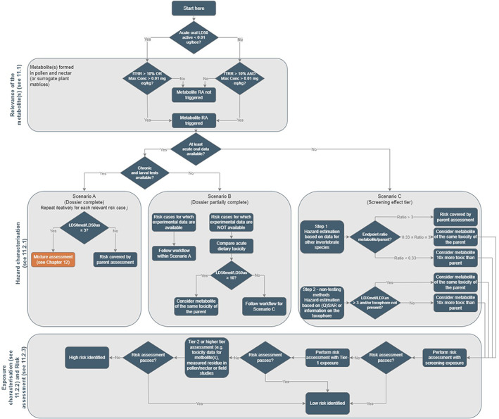
Flowchart for metabolite risk assessment
12. Mixtures
In this Chapter, an approach is proposed to address the risk of mixtures for honey bees, bumble bees and solitary bees with a focus solely on technical mixtures (products) containing more than one active substance and their co‐formulants undergoing an authorisation procedure. Bees may be exposed to other mixtures e.g. when the bee foraging activity across the landscape creates a mixture of PPPs at the hive/colony/nest (Knapp et al., 2023) or spray tank mixtures where different types of PPPs are mixed that may involve certain combinations of concern with potential for synergistic effects (e.g. pyrethroids insecticides and azole fungicides, (Siviter et al., 2021). While the concept and scheme proposed here is in principle also applicable to these mixtures, the respective exposure estimates of each of their components are a prerequisite for the mixture assessment that are not available in practice for these unknown mixtures. Besides, such combinations of substances are not expected within a technical mixture of active substance(s) and their co‐formulants undergoing an authorisation procedure according to Regulation (EC) 1107/2009, as those mixtures are intended for a specific use/target. Tank mixtures are therefore not within the scope of this guidance and not assessed in routine. Only when information is available for such combinations of substances (i.e. when a certain combination of PPPs is intended for tank mixing), the concept and scheme proposed within this Chapter may also apply.
12.1. Legal requirements
Regulation (EC) No 1107/2009 Article 29 requires that ‘interaction between the active substance, safeners, synergists and co‐formulants shall be taken into account’ in the evaluation and authorisation of a PPP. This explicitly refers to marketed PPP, which are, by origin, technical mixtures containing one to several active substances, plus, typically, several co‐formulants. Furthermore, the standard data requirements for PPP (Commission Regulation (EU) No 284/2013) request ‘any information on potentially unacceptable effects of the plant protection product on the environment, on plants and plant products shall be included as well as known and expected cumulative and synergistic effects’.
The following approach builds on existing methods and scientific experience in assessing chemical mixtures. In most cases, mixture effects are based on adding up the doses for common effects to estimate the overall risk. However, sometimes, the chemicals ‘interact’, meaning their toxicity increases or decreases. Therefore, the potential for interaction must be checked in order to capture greater than additive increased toxicity.
12.2. Risk assessment for mixtures
12.2.1. Defining the hazard
For the risk assessment (RA) of mixture under Regulation (EC) No 1107/2009, applicants and risk assessors should define which approach is more suitable for the hazard assessment. The hazard parameters to be used for the mixture assessment will be obtained from the data set built on data requirements (see Chapter 6). These data requirements are set irrespective of the mixture scheme below and will serve as the basis for the selection of the most appropriate approach. Two possible options are considered, which involve measured (‘whole mixture’ approach) or calculated (‘component based’ approach) mixture toxicity depending on the time frame of the exposure and the residue dynamics of the various components of the mixture. In some instances, the use of calculated mixture toxicity may better reflect the true mixture (not the PPP but the mixture ingested by bees via their diet) and should be considered whenever justified (i.e. a priori, no synergistic effects) and when this is the only possible approach (e.g. mixture composition of a.s. is different in the formulation than expected in the environment or experimental testing is technically not feasible). On another hand, the use of measured toxicity is more straightforward and already a current practice. The use of measured toxicity might then be considered for practicality, particularly in situations where no refinement of exposure parameters is necessary (e.g. for products of low risk) and also a fortiori considering that PPP studies are generally available for formulations with more than one active substance (see data requirements in Chapter 6). In some circumstances (e.g. low solubility), data for the active substances may be lacking and measured toxicity of the PPP can be used.
Then, in situations where no unacceptable risk is identified at screening step/Tier 1, based on measured toxicity of the PPP, no refinement of exposure parameters is necessary and the mixture risk assessment (presented below) can be bypassed.
On the basis of the mixture toxicity (measured or estimated) selected for each risk case (i.e. acute contact, acute dietary, chronic‐dietary and larvae‐dietary), a combined risk assessment can be conducted for each bee group, in line with the approach explained in Chapter 7. Since for the acute contact scenario bees are always exposed to the formulation (mixture) ‘as is’ (i.e. without any shift in mixture composition), the measured toxicity option should always be used for the acute contact risk assessment.
For the measured toxicity option, the selection of the relevant hazard parameters (DRCj) will follow the same rules as explained in Chapter 6.
There may be situations where the dose response of a mixture is not symmetric, e.g. if the different substances have very different slopes (refer to the example below) or are better described by different dose–response models. Whenever this is the case, the dose–response of the mixture may be characterised by an irregular shape with a shallower slope at lower doses and a steeper slope at higher doses. The opposite situation is not expected to occur.
Thus, for calculated mixture toxicity option, the potential asymmetry of the estimated curve renders the description of the dose–response less straightforward than it is for individual substances. In such cases, a formal description via 2/3 parameters is not always possible.
Under a dose addition (DA) approach, for a mixture of n components, a specific LDx,mix resulting in an effect level x is calculated as follows:
| (32) |
Where:
n: number of mixture components.
i: index from 1…n mixture components.
pi: the ith component as a relative fraction of the mixture composition (note: Σ pi must be 1).
LDxi: dose of component i provoking x% effect.
This means that when the dose–response relationships and the relative proportions of the n components of the mixtures are known, it is possible to calculate the LDx,mix for a range of effect levels. In this way, the dose–response of the mixture can be described relatively precisely (Figure 21).
Figure 21.
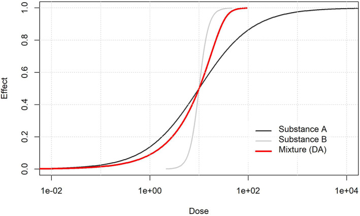
Illustration for a 1:1 mixture of substance A and substance B. Both DRCs of the substances are described by log‐logistic models, with the same LD50 of 10 (generic unit). The (red) curve describing the mixture is closer to Substance A in the left part of the plot, and then closer to Substance B in the right part. This is because the difference in the slope makes substance A the driver of the effects at lower doses and substance B the driver at higher doses. Despite the fact that the DRC of each component is described by a log‐logistic model, the asymmetry of the resulting curve makes it unsuitable to be described by the same model
To do this, it is proposed to calculate the mixture dose needed to achieve a suitable number of effect levels (i.e. from 1% to 99%) by using equation 1. Some minimum interpolations between the points would be needed. The resulting curve cannot be explained as a standard model, which means that it cannot be described by a simple combination of w parameters, but it can still be used to predict the effects caused by a certain exposure level to the mixture with reasonable accuracy.
12.2.2. Defining the exposure of the mixture to be assessed
The basic concept of the risk assessment for bees is that they are exposed to residues of active substances in the environment, e.g. via their food. Thus, the following steps refer to the assessment of effects from exposure to a mixture of active substances (and possibly also toxic co‐formulants) in the environment resulting from use of a formulation.
An LD50 for a mixture of active substances calculated assuming dose additivity can be conceived as an LD50 of a single virtual compound. It is thus deemed the most logical approach to also base the exposure side of the risk assessment on the same assumption. The substance content in the formulation and application rate per hectare should thus be expressed in terms of this virtual compound. The default residue dynamics used for both pollen and nectar (for each individual substance) are also applicable to the mixture as a single virtual compound.
However, if the dietary exposure assessment is refined using specific environmental fate data for individual active substances, the composition of the residues might change as compared to the original mixture. The exposure level PEQmix can be calculated as follows.
| (33) |
With:
PEQi = Predicted Exposure Quantity due to dietary exposure of active substance i, i.e. the intake of pesticide mass per bee. This is the output of the exposure estimation (see Chapter 5). It may include substance specific residue dynamics (e.g. refined RUD, refined dissipation half‐life, etc.).
It should be carefully checked whether metabolites of ecotoxicological relevance (see Chapter 11) have to be included into the PEQmix or not. For an initial screening approach, it may be assumed that the PEQi of all a.s. present in the formulation and the relevant metabolites that are formed from these substances will occur at the same moment and are not separated in time (i.e. worst‐case PEQmix). If, on this basis, the risk is not excluded, in a subsequent step a more detailed consideration of the predicted exposure patterns over time should be undertaken for the mixture RA. The ‘metabolite intake’ and the hazard parameters should be based on the risk assessment scheme for metabolites available in Chapter 11. This applies for both acute and chronic exposures.
A mixture toxicity risk assessment including metabolites should only be conducted if laboratory studies with the respective metabolite are available. Surrogate data based on non‐test methods or data on other invertebrate species should not be considered in a mixture assessment as, in case of failure, the use of extrapolation factors would render it difficult to discriminate the relative weights of the metabolite vs. its parent in the overall result. If laboratory studies are available for all risk cases (scenario A) and some of those present a toxicity similar or higher than the parent, then all endpoints should be used for the mixture assessment, not only those endpoints showing the same or higher toxicity compared to the parent. If laboratory studies are available for only some of the risk cases (scenario B), these endpoints should also be used for the mixture assessment, but only if one of the endpoints is of the same or higher toxicity compared to the parent (otherwise the risk of metabolite would be covered by the parent compound).
If the risk assessment is based on experimental toxicity data for the formulated product, no differentiation according to environmental fate parameters of individual active substances is possible. In principle, the concept of the single virtual compound could also be applied to calculate time‐weighted average concentrations (TWA) for mixtures or formulations. The default fate parameters used for individual substances also apply here.
Only active substances were used in the data set from which the default fate parameters of the dietary model are derived, then uncertainty remains as to the real fate of other co‐formulants present in the formulation. Co‐formulants may, in some cases, dissipate slower than the active substances and would not be covered by the PPP risk assessment at the screening and tier 1 level. In the absence of specific data for co‐formulants, uncertainty remains as to the actual exposure of bees to these compounds.
It is noted that the above considerations only concern dietary exposure, and not contact exposure, the latter being relevant only on an acute timeframe and estimated on the basis of a single application. Indeed, for acute contact (i.e. overspray), bees are always exposed to the formulation ‘as is’, without any shift in its composition.
12.2.3. Risk assessment scheme
A detailed step‐wise decision scheme is proposed below. Note that this scheme is not to be used to set the data requirements (see Chapter 6) but aims to provide guidance for the selection of the most adequate risk assessment approach (Figure 22).
Figure 22.
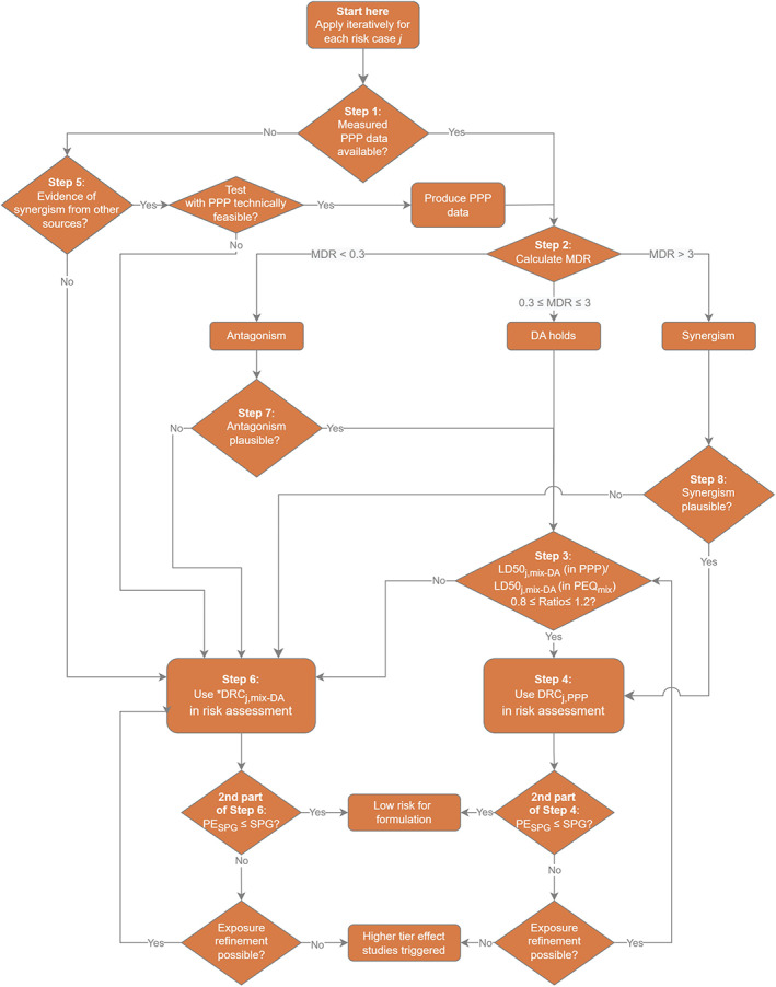
Workflow illustrating the risk assessment scheme for mixtures. *LD50,j,mix‐DA may need to be corrected by an appropriate Model Deviation Ratio (MDR) from other risk cases/species when synergism is plausible (see text in steps 5–6)
The selection of hazard parameters (DRCj) for each risk case j (i.e. acute, chronic, larval development) is based on the following scheme (to be applied iteratively for each risk case j, see Figure 16). Each of them can then be used in the combined risk assessment, whether based on measured or estimated toxicity.
Step 1. Are measured toxicity data (LD50j) with the formulation available for the given risk case (typically, when a PPP contains only one active substance, chronic data may be available only for the active substance, see Chapter 6)?
No, (Only data for the a.s. (LD50j a.s. ) are available): Go to 5.
Yes, (both data for formulation (LD50j PPP ) and active substance (LD50j a.s. ) are available: Go to 2.
Note that data on the entire dose–response are not required at this stage (endpoint selection only requires a comparison between measured and calculated LD50s, it does not require an assessment of effects based on estimated exposure levels).
Note for acute toxicity (dietary and contact), data are generally available for both the PPP and active substance(s). For data requirements, see Chapter 6 (Table 24).
Note that for formulations of low risk or when data are available only for the PPP (see data requirements in Chapter 6), a mixture assessment based on measured toxicity can be conducted and the following steps can be bypassed. In that case, no refinement of the exposure parameters should be used.
Step 2. Check the plausibility of the calculated mixture toxicity LD50j,mix‐DA assuming dose addition (DA) against the measured formulation toxicity (LD50j,PPP) on the basis of the mixture composition of the active substances in the formulation by means of the Model Deviation Ratio (MDR, see equation 3).
Notes:
In order to determine if the toxicity of the mixture is greater (i.e. potential synergism of toxicities) or lower (i.e. potential antagonism of toxicities) than expected according to DA, a comparison of the calculated LD50j,mix‐DA for the mixture composition of active substances in the formulation versus measured LD50j,PPP endpoints (expressed as the active substance content) is informative.
Thus, the first phase consists in estimating the mixture toxicity assuming the principle of dose addition (LD50j,mix‐DA, see equation 1).
At this stage, the intent is only to compare the calculated and the measured LD50j of the PPP, and not to compare those values to an exposure estimate (PEQ). Thus, information on the shape of the dose–response is not necessary at this stage.
This comparison may also indicate that other co‐formulants not included in the calculation contribute to the overall mixture toxicity in an appreciable way. When this is the case, they can be included in a refined calculation (if the respective single‐compound toxicity data are available). The possible outcome of the MDR calculation is the following:
| (34) |
0.33 ≤ MDR ≤ 3. The observed and calculated LD50j are considered to be in agreement if the MDR is between 0.33 and 3. This convention is in line with the recent EFSA recommendations related to pesticide risk assessment (Pesticide Peer Review Meeting 185, 9–12 October 2018 1 ). In relation to ‘when a formulation should be considered more toxic than the active substance’, the proposal was to account for a difference of a factor of three, as recommended in the guidance from the Directorate‐General for Health and Food Safety (SANCO/10597/2003 rev. 10.1) (European Commission, 2012) on the equivalence of batches. Thus, if the calculated MDR lies between these two values, it is considered that the DA hypothesis holds.
MDR is > 3. More‐than additive (i.e. synergistic) mixture toxicity is indicated if the MDR is > 3.
MDR is < 0.33. Less‐than additive (i.e. antagonistic) mixture toxicity is indicated if the MDR is below 0.33.
A careful interpretation of the MDR is mandatory, especially if not all components that potentially contribute to the observed mixture toxicity (e.g. co‐formulants) have been considered in the DA calculation. Care should also be taken that the counter‐checking of measured and calculated LD50j refers to the same basis, that is, the relative proportion of mixture components must be consistent (e.g. to the sum of active substances in a given PPP if co‐formulants are not included in the DA calculation).
If MDR = 0.33–3 (DA holds for the mixture): Go to 3
If MDR < 0.33 (mixture less toxic than DA): Go to 7
If MDR > 3 (mixture more toxic than DA‐potential synergism): Go to 8
Step 3. Check whether the mixture composition in the formulation study giving the measured mixture toxicity (LD50j,PPP) in terms of the relative proportions of the individual active substance is similar to the mixture composition of the PEQmix (PEQmix represents the mixture in the diet). This check is necessary only if exposure parameters were refined for one (or several) components of the mixture (no shift in their relative proportions would be expected otherwise). As a direct comparison on the basis of the relative proportions of the a.s. at the LD50j,PPP with the relative proportion at the PEQmix is not informative as such, the comparison is done based on calculated mixture toxicity (assuming DA) for both mixture compositions. Therefore, calculate LD50j,mix‐DA for the mixture composition of the a.s. of the PEQmix and compare with the estimate calculated for the formulation (as already done in step 2 above).
Note: For a meaningful assessment based on PPP measured toxicity (following step), it is crucial that the mixture at PEQmix does not differ too much from the original mixture (in the PPP). This step is necessary only if a shift in relative proportions of the individual compounds is expected i.e. if substance specific fate characteristics (e.g. DT50) are used. Otherwise, the default fate parameters apply to all compounds and no change is then expected in their relative proportions. This check between mixture compositions is considered necessary in case the tier 1 risk assessment fails and tier 2 is needed, which may require the refinement of fate parameters for acute and chronic risk assessment. It may be anticipated that a refined DT50 will have an impact on both the maximum expected residue level in case of multiple applications (and thus on the acute risk), as well as the average residue level over a prolonged exposure (and thus on the chronic risk). The comparison is performed based on calculated mixture toxicity (assuming DA) for both mixture compositions, that is, a calculation of LD50j,mix‐DA for the mixture composition of the a.s. of the PEQmix and comparison with the respective estimate calculated for the PPP. The relative proportion of a.s. is considered sufficiently similar if the outcome of these calculations deviates less than 20% (i.e. as already recommended in the guidance document for aquatic organisms). Hence, if LD50j,PPP (proportion of a.s. as contained in PPP) divided by LD50j,mix‐DA (proportion of a.s. at PEQmix) yields a value between 0.8 and 1.2, a direct comparison of PEQmix with the DRCj,PPP is feasible. If the mixture composition differs more profoundly the measured data cannot be used directly, however, they might be used to justify the use of the calculated approach. This check has to be performed for each proposed application in the GAP and for each organism, separately.
If LD50 j,mix‐DA (a.s. in PPP)/LD50 j,mix‐DA (a.s. in PEQ mix ) = 0.8–1.2 (mixture similar): Go to 4
If not (mixture not similar): Go to 6
Step 4. Use the measured mixture dose–response (DRCj,PPP) and proceed to the RA as described in Chapter 7.
Note: in case synergism is plausible (following step 8) this can only be accounted for by assuming that the relative proportion of the mixture components is fixed. A change in the mixture composition would likely be reflected in another, unknown, MDR value. Thus, when synergism is plausible, exposure refinements can only be considered if these do not cause a shift in the relative proportion (e.g. if refined DT50s are available for different components of the mixture, the worst case among them should be applied to all components).
PE SPG ≤ SPG: Low risk
PE SPG > SPG: low risk not demonstrated/check refinement options
Note that PESPG represents the combined effects of all the risk cases taken into consideration in the RA. To comply with the SPG, any risk case can be refined independently of the others and thus a refinement of another risk case may suffice.
Note that the use of measured mixture toxicity is recommended here for practical reasons but at this step the calculated mixture toxicity would generally lead to similar results (except in case of synergism).
Step 5. Is there evidence that synergistic interactions between mixture components might occur (e.g. based on toxicological knowledge from literature or from counter‐checking measured and calculated mixture toxicity for other risk cases/species) which cannot be ruled out for the given endpoint with sufficient certainty?
Note: if synergistic effects cannot be excluded, the risk assessment should preferably be based on measurements, as synergistic interactions are not predictable by DA nor by other concepts such as independent action/response addition. If experimental testing of the mixture is not an option (e.g. for technical reasons) for certain species and endpoints, but synergism is known from other studies, the RA may be performed by shifting the calculated DRC j,mix‐DA by the MDR obtained from other risk cases/species.
Yes (mixture toxicity calculation not feasible): Measured mixture toxicity data required for RA
If measured mixture toxicity becomes available: Go to 2
If measuring the mixture toxicity is not technically feasible, but a reliable MDR is available from other risk cases/species, shift the calculated DRCj,mix‐DA by the MDR and go to 6
No (mixture toxicity calculation feasible): Go to 6
Step 6. Use the calculated dose response curve (DRCj,mix‐DA) to estimate the effect for the risk case of concern and proceed to the RA.
Note: If synergism is plausible this can only be accounted for by applying an appropriate MDR (see step 5). The use of the MDR, however, only works if the relative proportion of the mixture components is fixed. A change in the mixture composition would likely be reflected in another, unknown, MDR value. Thus, when synergism is plausible, exposure refinements can only be considered if these do not cause a shift in the relative proportions (e.g. if refined DT50s are available for different components of the mixture, the worst case among them should be applied to all components).
Note that relevant metabolites are assessed as a mixture together with the parent compounds (see Chapter 11) using DA.
PE SPG ≤ SPG: Low risk
PE SPG > SPG: Low risk not demonstrated, check single‐substance refinement options
Note that PESPG represents the combined effects of all the risk cases taken in consideration in the RA. To comply with the SPG, any risk case can be refined independently of the others and thus a refinement of another risk case may suffice.
Note that it is not recommended to base the risk assessment on an eventual driver substance (i.e. when toxicity is largely explained by the toxicity of a single a.s.). This is because the toxic driver also depends upon the assumed mixture composition, which may be different for a PPP as formulated and the assumed mixture composition at PEQmix (due to different degradation rates of different components). Defining a driver may be complex and it is not always necessary, thus it is not recommended for screening/Tier 1 steps. However, under some circumstances, the use of a driver may still be considered when single active substance higher tier data (i.e. an effect field study) are available for a toxic compound. If it can be clearly demonstrated that the other compounds do not contribute to the overall toxicity (either by additive effect or synergism), single active substance higher tier data may potentially be used to address the risk of the PPP.
Step 7. Carefully recheck the apparent antagonism as observed in the measured mixture toxicity data (DRCj,PPP) regarding potential impacts of the default assumption of DA (check for heterogeneous input data i.e. different study designs/endpoints). Does the apparent antagonism hold?
Note: If plausible toxicological explanation for this apparent antagonism can be provided (e.g. special feature of the formulation type), the RA should be based on the measured toxicity. Otherwise, the calculated mixture toxicity is a better option. No correction for MDR is needed, as the calculated mixture toxicity represents a worst case.
Yes (i.e. antagonism holds): Go to 3
No (i.e. antagonism does not hold): Go to 6
Step 8. Carefully recheck the apparent synergism as observed in the measured mixture toxicity data (DRCj,PPP) regarding potential impacts of heterogeneous input data (testing conditions/endpoints should be homogeneous) and of co‐formulants ignored in the DA calculation. Does the apparent synergism hold?
Note: If plausible toxicological explanation for this apparent synergism is available or if this check reveals the presence of a toxic co‐formulant, the RA should be based on the measured toxicity. Otherwise, the calculated mixture toxicity is a better option.
Yes: Go to 4
No: Go to 6
13. Risk mitigation measures
13.1. Introduction
If a high risk to honey bees, bumble bees and/or solitary bees is indicated at lower tier (i.e. Tier 1, Tier 2) or higher tier, an option to address and manage the risk is to consider risk mitigation measures to reduce the exposure of bees. Such measures can be proposed by the applicant with the submission of the dossiers and, ideally, quantitative data to prove the reduction of exposure as well as a clear description of the measure with respect to representative use should be submitted.
In fact, if it becomes clear that certain measures are needed to ensure higher protection of bees, restrictions can be set at approval (or renewal) of substances at EU level and/or at the authorisation of PPPs at MS level by risk managers.
It should be noted that changes to the GAP during EU level assessments are not allowed and therefore applicants should carefully consider their range of selected GAPs when developing a dossier.
13.2. Target risk mitigation measures
Target mitigation measures are needed to mitigate the identified risk due to PPP exposure. It is important to note that those mitigations should sufficiently reduce the risk to a level which is considered to be in line with the agreed SPGs (i.e. a low risk using a refined exposure estimate considering the mitigation must be demonstrated). As such any suggested mitigation must be accompanied by an appropriate risk assessment for which additional data may be needed.
Measures which reduce exposure would lead to refined PEQj values at the Tier 1 or Tier 2 (see Sections 3 and 5). In general, by implementing specific reduction exposure measures potential repercussions on other sections, especially on efficacy, must be taken into account.
Targeted measures could cover (list not exhaustive):
Drift reduction technique for spray applications (e.g. nozzles, buffer zones, deflectors) or a higher quality of treated seeds to reduce the exposure estimation for the field margin/adjacent crop scenarios;
Specific technologies to reduce the exposure to flowering weeds in the field;
- Targeted representative uses (GAPs) that would allow to reduce and/or avoid the exposure such:
- Restrictions on growth stage e.g. outside the flowering crop period;
- Restrictions to permanent greenhouses;
- Reduction of application rate/number of applications and/or increase of interval between applications;
- Localised applications.
When imposing risk mitigation measures, it is important to consider that they are effective to address the identified concern and ensure they are practicable and enforceable.
Regarding the protection of bees, specifically to managed honey bees, Regulation (EU) No 547/201113 provides a set of ‘risk phrases’ aimed at reducing the exposure during and following PPP treatments. It is important to note that the Regulation 547/2011 is currently under revision; therefore, the current risk phrases might be revised and/or new ones may be added. Furthermore, under the Sustainable Use Directive14 (which is also under revision) additional provisions to the use of a PPP can be assigned by MS according to the Good Agricultural Practices.
13.3. Developing risk mitigation measures
There is increasing support for that local access to a diversity of flower resources can reduce bee exposure to PPPs and resulting effects on bees based on both semi‐field (Stuligross and Williams, 2020; Ingwell et al., 2021; Klaus et al., 2021; Wintermantel et al., 2022) and field (Rundlöf et al., 2022) studies. Establishment of local flower plantings could thus be a risk mitigation measure for testing and development by applicants. Such development would, however, not only include challenges related to quantification of the risk reduction but also related to communication and enforceability.
In addition, different initiatives (e.g. PERFECTLIFE15, OPTIMA16) at the European level have collected information on reduction exposure measures and on the percentage of exposure reduction that they can achieve.
A SETAC publication titled ‘Mitigating the risks of plant protection products in the environment, MAgPIE’ (Alix et al, 2017) was published following the workshops held in 2013. The aim of the workshops was to produce a toolbox of risk mitigation measures which can be used in a quantitative risk assessment for bees. Even though the outcome of these workshops is not endorsed some examples of proposed mitigation measures are presented below. It is important to highlight that the proposal from the MAgPIE report should be considered as indicative.
14. Conclusions
The review of the EFSA (2013) has been performed in line with the ToRs of the mandate. In particular with this document the list of bee attractive crops was reviewed, in consideration to the growing phases of the crop and the agricultural practices (harvesting time or after flowering). Furthermore, the relevance of guttation, and in general collection and use of water was reconsidered. The relevance of the exposure scenarios was reviewed and the methodologies for exposure and hazard assessment were updated for all the bee groups. A comprehensive review of the evidence for bee background mortality was provided in a standalone document. For risk assessment, a combined approach which integrates the different risk cases (i.e. acute‐contact, acute‐, chronic‐ and larvae‐dietary) was proposed. This is operational only for honey bees, but it will be applicable for bumble bees and solitary bees when a defined threshold of acceptable effects is provided by risk manages. The requirements for higher tier studies, including considerations for the statistical requirements, were reviewed and further elaborated. Population‐level modelling of effects for different ecological and agricultural practice scenarios were considered as part of the higher tier risk assessment. However, no specific recommendations were included since such models first would need to be developed, calibrated and evaluated for their use in regulatory bee risk assessment. Feedback from stakeholders and MSs was duly considered as well as ongoing activities initiated by the European Commission throughout the whole review process.
15. Recommendations
The WG recommends that the areas not covered in this guidance are addressed in future activities and recognises the need to generate further research and data. These are listed below, in this section.
Generally, the WG recommends updating the parameters used in this guidance document which are based on other guidance documents when those are revised after the publication of this guidance.
Inclusion of potentially important matrices/exposure routes/life stages
There are multiple environmental matrices (e.g. resin, wax, honey dew, extrafloral nectar, soil;) that can be contaminated by PPPs which bees may encounter that are not covered in this guidance document. These may need to be incorporated in future risk assessment scheme. However, it is important to note that simply detecting a PPP in a matrix is not sufficient to include that matrix in a risk assessment. The issues highlighted for the water scenario, discussed in Annex E of supplementary document, provide one example of the difficulties in incorporating potentially relevant exposure routes into risk assessment where there is insufficient information to develop risk assessment scenarios or methodology.
Further consideration is needed for exposure and hazard characterisation due to inhalation for highly volatile PPPs.
Further research is needed to allow including bumble bee queens in the risk assessment (see for more details supplementary document 3.2.3.2) and to address reproductive effect on honey bee queens and drones.
Exposure assessment
The exposure assessment is based on the knowledge and best scientific practice available at the time of writing the guidance document. Nevertheless, further research may improve the parameter values chosen in Tier 1. Specifically, the WG recommends further research on the following topics:
To improve the realism of crop interception, spray and dust drift deposition estimations (see more for details Section 5.2.2.1 of the supplementary document);
To investigate the residue behaviour of PPPs in plants leading to potential contamination of pollen and nectar after pre‐flowering application, both for spray and solid formulations;
To investigate further the growth pattern of the crop grown in the EU and link BBCH stages to calendar days;
To address the knowledge gaps regarding the food consumption of bees and bee larvae (see more for details supplementary document 5.3.5);
To analyse (or expand) available data on RUD values in attractive weeds and crops resulting from spray applications to underpin the hypothesis that the RUD of a substance in attractive weeds can be predicted from the RUD in treated crops;
To analyse (or expand) available data on concentrations in nectar and pollen that result from exposure to dust drift (originating both from seed treatments and granules) in order to assess how these data relate to concentrations in nectar and pollen that result from exposure to spray drift and next, to evaluate the assumptions used in the current guidance document;
To further investigate factors responsible for the pesticide dissipation in/on plants and the variability between substances, plant species, matrices, study‐specific environmental conditions, sampling procedure, sampling processing, pesticide application and doses;
To improve biological/ecological knowledge on all the species in the bumble bee and solitary bee groups, especially for larvae (such as time needed for the preparation of the provision, length of larval development) or the residue behaviour in the provision, to allow a more realistic proposal for the time window parameter for these bee groups;
To develop a list of likely rotational crops in order to improve the realism of the annual succeeding crop scenario;
Currently, the use of any physico‐chemical property or a combination of them to set a screening tool for the succeeding crop scenario is not recommended and may deserve further consideration only once the relevant OECD Test Guideline (OECD, 2021b) is adopted and published, and an EU harmonised approach on how to deal with the plant uptake factor/TSCF has been established;
To further assess the abundance of weeds in flower, which could improve the risk assessment for the weed scenario (see chapter 7 of Annex D to the supplementary document). Further data is also needed to potentially revise the threshold value for the significant fraction of weeds within a single field (see chapter 2 of that Annex D);
To investigate additional methods to determine the PPP dissipation rate in honey (see more for details Section 7.2.3 Annex G to the supplementary document;
To investigate the proportion of food consumed by the bees that is contaminated with PPPs in order to optimise the various exposure scenarios and calculate the total daily intake of PPPs the various exposure scenarios and calculate the total daily intake of PPPs.
In addition, the development of appropriate exposure estimation methodologies for methods of application other than spray, granules and seed treatments requires is needed.
Effect assessment in lower tiers
Standard ring‐tested ecotoxicity protocols are currently limited to honey bees, and bumble bee species. This limits the potential to experimentally verify differences in physiological sensitivity among bee species. A limited number of tests exist in the literature with non‐standard species but are almost exclusively limited to acute contact assays. The WG highlights parallel needs for future research:
To develop standardised, validated protocols for widening the current set of agreed OECD tests. Particularly, the need to perform dietary chronic and larval tests with non‐Apis bees should be considered a high priority;
To develop methods to accurately test or predict the toxicity of active substances to different bee taxa. Methods relying on the molecular structure/mode of action of the chemicals as well as specific bee traits appear promising. While the development of new effect assessment methods, such as the use of transcriptomics or biochemical tests, is required, those methods that do not directly measure endpoints with a clear link with the attribute defined in the SPG, need to undergo extensive validation to translate the effect assessment to an effect on colony/population size;
Mechanistic models like those developed for deriving extrapolation factors (Tef) in the guidance document will likely play an important role. While they are limited by the paucity of experimental information in accounting for differences between bees, they may nonetheless reveal patterns related to toxicokinetic and toxicodynamic processes that can increase confidence in extrapolation. Among the lines of research focusing on mechanistic explanation of the toxicity, developments of methods investigating the genetic and molecular basis of the inter‐species sensitivity (Manjon et al., 2018; Hayward et al., 2019) have recently shed light on unexpected sensitivity patterns. This approach is particularly promising, as techniques for mapping the genome are improving at a fast pace.
Lower tier risk assessment
The WG recommends investigating:
the impact (any model‐based or empirical research) of the extrapolation from individual to colony level/population level, including the conservativeness of this extrapolation method. For modelling studies, the definition of appropriate environmental scenarios is key and should be carefully designed;
how at colony levels effects on adult bees via the two different exposure routes of contact or diet, and via diet on larvae combine to corresponding colony‐level impacts. For modelling studies, the definition of appropriate environmental scenarios is key and should be carefully designed.
These are discussed further into Chapter 7 of the supporting document.
Sublethal effects on honey bees in risk assessment
The assessment described here represents a preliminary attempt at introducing sublethal effects assessment into risk assessment for bees within the EU. However, it is important to recognise that the three main criticisms of the methods that prevented the inclusion of a more extensive sublethal effects assessment in EFSA 2013 still apply. Therefore, the WG recommend the following:
There is currently no link between the observed sublethal behaviours and the SPG, therefore the biggest outstanding challenge to overcome is linking sublethal effects to the SPG or developing targeted SPGs for sublethal behaviour;
While the current sublethal effects assessments can detect large differences in behaviour induced by pesticides they require regular human observations. The development of standardised protocols which minimise observer bias, with minimal additional experimental burden, and accurately quantify the behaviours should be a priority;
Finally, while this initial guidance for sublethal effects assessment focusses on honey bees, standardised sublethal effects assessments should also be developed for bumble bees and solitary bees.
These are discussed further into Section 9.1 of the supporting document.
Higher tier risk assessment
The goal of the risk assessment is to assess the risk to all bee species which may be exposed to PPP. This is explicitly dealt with at the lower tier, while at the higher tier this is not yet possible, due to the current experimental limitations to a few manageable species and life stages and lack of methodology to extrapolate the outcome of higher tier studies across species and populations and even to pollination. This is considered one of the main areas where further research is needed and where a combination of experimental approaches, mechanistic models and monitoring techniques are likely to provide future opportunities (e.g. Uhl and Brühl, 2019; Topping et al., 2021; Siviter et al., 2023):
The WG suggests exploring approaches for extrapolation from the tested species to whole group of bees, e.g. bee species richness. This includes the development of ecological models to support extrapolation to non‐standard solitary or bumble bee species, and also relates to the role of monitoring in ERA, which is not part of the current guidance;
Development of protocols for other species than Bombus terrestris and Osmia bicornis/cornuta is needed;
There is an urgent need to better support the SPGs for bumble bees and solitary bees. For example, developing modelling techniques similar to those available for honey bees and work with colony and population data to explore variability and possible normal operating ranges for the relevant endpoints (EFSA, 2022);
The WG recommends the implementation and evaluation of complex honey bee colony models under different environmental scenarios for use in the regulatory environmental risk assessment (see Chapter 10.6). The same holds for colony or population models for any other bee species. Such evaluation should be performed following general and specific criteria by expert groups ideally at EFSA level;
Monitoring initiatives, e.g. suggested EU Pollinator Monitoring Scheme (EU‐PoMS; Potts et al. 2020), the Monitoring of Biodiversity in Agricultural Landscapes (EMBAL) and using honey bees as bioindicators to monitor pesticides and other pollutants (e.g. INSIGNIA), are suggested to be explored for SPG developments, feeding into model validation and form the basis for supporting a follow up of the risk assessment as well as risk management decision consequences.
Further improvement of the study methods proposed in this guidance is also needed:
Annex B, chapter 10, suggests some methods for refining contact exposure. Since very little experience has been gained so far with this type of field exposure study, the WG recommends developing further guidance in future;
Annex C, Section 4.3.5 describes how in semi‐field tests with honey bees, forager mortality is counted on sheets and then extrapolated to the total area of the cage surface. To improve this methodology, further knowledge on the ratio of mortality on sheets and crop area would be useful;
Annex C, Section 4.4, describes how further research may justify other endpoints than the currently used ‘amount of capped brood’ for the evaluation of brood effects in the honey bee colony feeder study;
The WG considers the large‐scale colony feeding study (LSCF; e.g. Overmyer et al., 2018), which is currently used in North American bee risk assessment, a promising study design for honey bees. Once more data are available and experience has been gathered, its potential use in European bee risk assessment should be evaluated;
If higher tier studies are needed for substances that show TRT properties, it is recommended in the guidance document to include also the overwintering period in these studies. It was pointed out during the public consultation on the draft guidance document that the results for overwintering are variable, and therefore difficult to interpret. Therefore, further research is needed on how studying overwintering success of honey bee colonies can be improved;
Further development and ring‐testing of study protocols are needed for Bombus terrestris and Osmia bicornis/cornuta;
Further research on and experience with novel observation methodologies (e.g. bee counter or video recording at the hive entrance, RfID technology, digital photography, hive weighing, etc.) is recommended.
Metabolites
The WG recommends improving QSAR toxicity estimations for bees, as detailed in Appendix C.
Mixtures
In addition to the recommendations included in EFSA Scientific Committee (2019), the working group recommends further investigations for the fate and behaviour of co‐formulants in pollen and nectar.
Abbreviations
- a.s.
Active substance
- ac
Acute
- AF
Assessment Factor
- AR
Application rate
- AUC
Area under the curve
- BB
Bumble bee
- BBCH
Biologische Bundesanstalt, Bundessortenamt and Chemical industry
- BC
Broadcasting of seed or granule
- be
Before flowering
- BSF
Body surface factor (dm^2/bee)
- bw
body weight
- CAT
Critical Appraisal Tool
- ch
Chronic
- CLP
Classification, Labelling, Packaging
- CMP
Food consumption, e.g. CMPsu: sugar consumption
- cn
Contact
- CONC
Concentration
- CRO
Contract Research Organisation
- Ctgb
Dutch Board for the Authorisation of Plant Protection Products and Biocides
- d
day
- DA
Dose addition
- DAR
Draft Assessment Report
- di
Dietary
- DTx
Half life parameter e.g. DT50po residues halving time in pollen
- du
During flowering
- DW
Downward
- EC
European Commission
- ECPA
European Crop Protection Association
- EDx
Effect dose, e.g. ED50 Effect dose for 50% of the organisms tested
- EED
Estimated exposure dose (in higher tier effect studies)
- EF
Exposure factor
- EfAGs
Effect Assessment Goals
- EFSA
European Food Safety Authority
- EPPO
European and Mediterranean Plant Protection Organisation
- ERA
Environmental Risk Assessment
- ERC
Environmental Relevant Concentration
- EU
European Union
- ExAGs
Exposure Assessment Goals
- FOCUS
Forum for the Co‐ordination of pesticide fate models and their Use
- GAP
Good Agricultural Practice. Often used to refer to the representative/proposed use of an a.s. or PPP (e.g. applications rate, timing, growth stage etc)
- GD
Guidance Document
- GLP
Good Laboratory Practice
- gw
Ground water
- HB
Honey bee
- ho
Honey
- i
Interval between multiple applications
- ICPS
International Centre for Pesticides and Health Risk Prevention
- IUPAC
International Union of Pure and Applied Chemistry
- JRC
Joint Research Centre
- KOC
Organic carbon absorption coefficient
- KOW
Octanol–water partition coefficient
- LCx
Lethal concentration, e.g. LC50 median Lethal Concentration
- LDDx
Lethal Dietary Dose, e.g. LDD50 median Lethal Dietary Dose
- LDx
Lethal dose; the dose at which x % of the test organisms die.
- LOD
Limit of detection
- LOEAL
Lowest observed adverse effect level
- LOQ
Limit of quantification
- lv
Larvae
- MAF
Multiple application factor
- MoA
Mode of Action
- MRL
Maximum residue levels
- MS
Member State
- mt
Metabolite
- n
Number of application, e.g. the number of applications before flowering (nbe) and the number of applications during flowering (ndu)
- ne
Nectar
- NOEC
No Observed Effect Concentration
- NOED
No observed effect dose
- NOEDD
No Observed Effect Dietary Dose
- NOEL
No observed effect level
- OECD
Organisation for Economic Co‐operation and Development
- OPPTS
US EPA's Office of Pesticide Programs and Toxic Substances
- PCUD
Predicted Concentration per Unit Dose
- PEC
Predicted environmental concentration
- PEQ
Predicted exposure quantity
- PFF
Pre‐flowering factor
- pl
Plant
- po
Pollen
- PPBD
Pesticide Properties Database
- ppm
Parts per million
- PPP
Plant Protection Product
- PPR Panel
EFSA Scientific Panel on Plant Protection Products and their Residues
- pr
Parent
- QSAR
Quantitative structure–activity relationship
- RA
Risk assessment
- RAR
Renewal Assessment Report
- RM
Risk manager
- RMS
Rapporteur Member State
- RUD
Residue per unit dose
- SANCO
European Commission Health and Consumer Protection Directorate General
- SB
Solitary bee
- SETAC
Society of Environmental Toxicology and Chemistry
- SN
Sugar content of nectar
- so
Soil
- SPG
Specific protection goal
- SSD
Species Sensitivity Distribution
- su
Sugar
- SUW
Sideward, Upward
- SV
shortcut value
- sw
Surface water
- ToR
Terms of Reference
- TRR
Total Radioactive residue
- TRT
Time‐reinforced toxicity
- TWA
Time weighted average
- US EPA
United States Environmental Protection Agency
- USDA
United States department of Agriculture
- w
Time window for deriving time‐weighted average concentrations for chronic exposure
- WG
Working Group
- wi
Winter
- WoE
Weight of evidence
Glossary
- Abundance
The total number of individuals of a taxon in an area
- Acute toxicity
Responses caused by short‐term exposure to a toxicant
- Adsorption
The adhesion of a substance (e.g. active ingredient of a plant protection product) on the surface of solids or fluids
- Alloethism
A common mechanism of task specialisation in eusocial colonies is alloethism, in which workers perform different tasks allocated by body size
- Background mortality
Mortality rates observed in stands in the absence of severe disturbances
- Brushing
Application of a liquid product or powder with a brush
- Buffer strip
in‐field; non‐treated cropped or non‐cropped zone of a defined width at the edge of a field that is influenced by the farmers action (e.g. spray drift). The buffer strip is normally enforced by authorities and underlies prescribed actions in order to meet the off‐field SPG. In addition, buffer strips may provide a recovery potential for the cropped area
- Colony
A colony consists a number of individuals of the same species that are living in close association with each other.
- Colony strength
Colony size, defined here as the number of adults that forms the colony
- Degradation
Loss process by which a substance is physically transformed from one chemical species to another. This can ultimately result in the formation of unextracted residues and CO2, but not necessarily in all cases
- Deterministic model
A mathematical model in which all the relationships are fixed and the concept of probability is not involved
- Dipping
Application by immersing the treated object or part of it in a liquid product or solution
- Direct effect
An effect that is mediated solely by the interaction between a specified ecological receptor and an environmental stressor.
- Dissipation
Result of one or more loss processes leading to the disappearance of a substance from an environmental matrix, e.g. soil. Loss processes contributing to dissipation include degradation within the soil matrix by biotic and/or abiotic processes, soil surface photolysis, volatilisation, plant uptake and leaching
- Dust drift
Drift of solid particles released during non‐spray applications (seed treatments or granules)
- Dusting
Application of a product by blowing tiny solid particles (dustable powder) towards the treated object
- Ecosystem
A dynamic complex of plant, animal and microorganism communities and their non‐living environment interacting as a functional unit.
- Ecotoxicologically Relevant Exposure Quantity (EREQ)
Conceptual interface between the effect and exposure‐tiers. It is based on ecotoxicological considerations and defines the type of exposure quantity that in a mechanistic sense best explains observed effects in an ecotoxicological experiment
- Effect Assessment Goal (EfAG)
The EfAG operationalises the Specific Protection Goals with respect to the effect assessment, e.g. definition of relevant model species, type of toxicity, measured endpoints for the relevant species, extrapolation between species.
- Environmental risk assessment (ERA)
A scientifically based process consisting of four steps: hazard identification, hazard characterisation, exposure assessment and risk characterisation
- Estimated Exposure Dose (EED)
Estimated exposure in effect field studies.
- Eusocial, eusociality
A social colonial existence, where adult colony members belong to two or more overlapping generations, care cooperatively for the young, and are divided into reproductive and non‐reproductive (or at least less‐reproductive) castes. Both honey bees and bumble bees are eusocial.
- Expert Knowledge Elicitation (EKE)
A systematic, documented and reviewable process to retrieve expert judgements from a group of experts, often in the form of a probability distribution
- Exposure Assessment Goal (ExAG)
The ExAG operationalises the Specific Protection Goals with respect to the exposure assessment in the environment, e.g. definition of the environmental exposure, type, duration, matrix and level of conservativeness of the exposure estimate.
- Exposure estimation
The exposure estimation in the different tiers will provide PEQ for each of the above risk cases and it is indicated as PEQj, where the subscript j indicates risk cases.
- Exposure scenario
The scenarios define where bees may encounter PPPs or contaminated matrices either in areas treated with the PPP (in‐crop) or in areas which were not directly treated but have been unintentionally contaminated (off‐crop areas).
- Exposure via contact
Occurs when bees enter in physical contact with the PPPs or with contaminated matrices, but does not involve ingestion.
- Exposure via diet
Occurs when bees orally consume contaminated material and therefore, they ingest residues of PPPs with their diet.
- Extrafloral nectaries
Specialised nectar‐secreting plant glands that develop outside of flowers and are not involved in pollination
- Fogging
Application of a product by producing an atmosphere full of tiny droplets (particle size 0.05–50 μm)
- Fumigating
Application of a product that completely fills a confined space in a gaseous form
- Guttation
Exudation of drops of xylem sap on the tips or edges of leaves of some vascular plants
- Hive
Enclosed, man‐made structure in which some honey bee or bumble bee colonies with their nets are kept.
- Home range
The area, usually around the domicile, over which an animal normally travels in search (e.g. of food)
- Honey dew
A sugary secretion produced by aphids and other insects
- Impregnating
Application of a liquid product or solution for absorption by a solid object
- In‐crop area
Surface covered by the crop plants including the space between the crop rows.
- Indirect effect
An indirect effect involves effects due impact of PPPs on bees habitats and food availability.
- In‐field area
The crop area and its boundaries that are managed by the farmer in the context of crop management.
- Injecting
Application of a liquid product or solution by injecting it directly into the treated object
- Landscape factor (LF)
This factor describes the proportion of the food intake of a bee colony or population that originates from the treated field: e.g. LFpo landscape factor for pollen
- Line of evidence
A set of relevant information of similar type grouped to assess a hypothesis. There is no fixed rule on how much similarity of the information is required within the same line of evidence. This is for the assessor(s) to decide, and depends on what they find useful for the purpose of the scientific assessment.
- Metabolite
A substance made or used when a parent substance (or compound) is broken down
- Metapopulation
An overall population comprising populations of the same species connected through immigration and emigration.
- Mixture (Technical)
Mixture (products) containing more than one active substance and their co‐formulants, undergoing an authorisation procedure
- Multivoltine
Referring to organisms having multiple generations per year
- Nest
A nest is a structure built by the bees to hold eggs, offspring and the adult form(s) itself. Honey bees, bumble bee and solitary bees can have nest(s).
- Niche
The ecological role of a species in a community
- Off‐crop area
Any uncropped area. It includes also uncropped areas in‐field, and such areas can be, e.g. the minimal required zone for agricultural management, buffer strips or beetle banks.
- Off‐field area
Area surrounding a field; either (semi)natural habitats with high ecological value (such as hedgerow or grass strip) or simple structures (fence or a bare strip of land); normally no short‐term changes in cultivation, in most cases not to be influenced by the farmer. Another off‐field category comprises man‐made structures, e.g. an adjacent field, roads, etc.
- Parameterisation
Parameter definition, the process of defining parameters that are used to represent the (biological) processes in a model
- Polyethism
A common mechanism of task specialisation in eusocial colonies is age or temporal polyethism, in which workers perform different tasks as they age
- Population
A group of individuals of the same species.
- Proprietary studies/dossier studies
Studies which are performed to support a dossier of an active substance or plant protection product and which are not freely accessible.
- Protection goals
The objectives of environmental policies, typically defined in law or regulations.
- Recovery
Ecological recovery is the return of the perturbed ecological endpoint (e.g. species composition, population density) to its normal operating range.
- Relevance
The contribution a piece or line of evidence would make to answer a specified question from a regulatory, biological and /or exposure point of view
- Reliability
The inherent quality of a piece of information, particularly considering the experimental procedure and the resulting plausibility of the findings.
- Residue Unit dose (RUD)
The parameter expressing the residue concentration of the pesticide molecule in pollen and in nectar, standardised on an application rate of 1 kg/ha
- Risk Mitigation Measure (RMM)
Actions which are needed to mitigate/manage a risk to bees due to pesticide exposure
- Sensitivity analysis
The quantification of the effect of changes in input values or assumptions (including boundaries and model functional form) on the outputs. By investigating the relative sensitivity of model parameters, a user can become knowledgeable about the relative importance of parameters in the model
- Shortcut value (SV)
The 90th percentile of a distribution of residue intake per bee (or larvae) over a colony (or population, for solitary bees).
- Species diversity
The number of different species/taxa within a given community
- Species sensitivity distribution (SSD)
Models of the variation in sensitivity of species to a particular stressor. They are generated by fitting a statistical or empirical distribution function to the proportion of species affected as a function of stressor concentration or dose. Traditionally, SSDs are created using data from single‐stressor laboratory toxicity tests, such as median lethal concentrations (LC50s).
- Spray drift
Drift of liquid particles applied via a spray boom
- Synergism
Activity of two or more chemical agents given together that is greater than the sum of activity had the agents been given separately.
- Threshold
The minimum level of a value of a stimulus to elicit a response
- Time‐Reinforced Toxicity (TRT)
The potential of the compound under evaluation for showing increased toxic effects due to long‐term exposure to low doses, compared to what would be expected based on short‐term exposure to higher doses
- Toxicity extrapolation factor (TEF)
Extrapolation factors from standard species to smaller bumble bees and solitary bees for a generic (substance‐independent) relationship between LD50 and bee weights
- Toxicodynamics
All processes that lead to the damage and/or mortality of the organism exposed to toxic compounds. Biological effects are caused by the toxic compounds on the molecular level, where the molecules of the toxic compound interfere with one or more biochemical pathways. Toxicodynamic part of TKTD models integrate all those processes into only a few equations that capture the dynamics of responses or effects over time.
- Toxicokinetics
All processes that influence the dynamics in internal exposure of an individual to the toxic compound, and include absorption, distribution, metabolism and elimination. Toxicokinetic models are used to estimate internal exposure concentrations.
- Trait
A well‐defined, measurable, phenotypic or ecological character of an organism, generally measured at the individual level, but often applied as the mean state of a species.
- Uncertainty analysis
Analysis of all factors that could reduce the appropriateness and precision of a model to describe a certain phenomenon
- Uncertainty
Uncertainty is the inability to determine the true state of affairs of a system and it may arise in different stages of risk assessment due to lack of knowledge and to natural variability.
- Univoltine
Referring to organisms having a single generation a year
- Weight of evidence assessment
A process in which evidence is integrated to determine the relative support for possible answers to a question
Appendices to the guidance document
Appendix A – List of crop attractiveness for pollen and nectar
1.
This appendix includes the revised list of crop for their attractiveness to bees for pollen and nectar. It is available as an Excel spread sheet.
Appendix B – Parameters for contact and dietary exposure
1.
This appendix includes the parameters for contact and exposure estimation for honey bees, bumble bees and solitary bees. It is available as two separate Excel spread sheets.
Appendix C – Additional information for metabolite risk assessment
C.1. Introduction
This appendix proposes guidance for conducting the metabolite risk assessment for bees in the EU regulatory context. The main objectives of this appendix are:
To provide further information on available source for residue data in pollen and nectar and
To provide further guidance on how to use non‐test methods (e.g. QSAR).
C.2. Sources for residue data in pollen and nectar
Ideally the risk assessment for metabolites should be based on data from residues studies of the relevant matrices (pollen and nectar). Therefore, there is a need to ensure that the relevant available information in the dossier is identified by the applicant and risk assessor.
Residues in pollen and nectar resulting from the use of the active substance are addressed by different studies. Each metabolite identified at or above 10% TRR and/or 0.01 mg eq/kg in these specific studies can be considered relevant.
Residue studies in (surrogate) crops in pollen and nectar
Residue studies are intended to provide information on the major degradation products of the applied substances and to measure the residues of the active substance and its degradation products in the relevant matrices pollen and nectar. The submission of a residue trial for pollen and nectar is not a standard data requirement but is the most appropriate approach addressing the identification of relevant metabolites in pollen and nectar matrices. According to the data requirements for plant metabolism studies (Section 6 of Regulation (EC) No 283/2013), residue trials should be performed according to the proposed critical GAP. The test conditions (maximum number of applications, shortest interval between application and maximum application rate) should be considered to identify the highest residues which may reasonably arise and should be representative of the realistic conditions of the critical GAP. The same assumptions can also be made for the metabolites formed in the matrices pollen and nectar. It may not be practical to test all crops in which the product is proposed to be used. As a worst‐case approach, the submission of a residue trial performed in a surrogate flowering crop (e.g. Phacelia, oilseed rape or sunflowers) might be considered for the purpose of identification of relevant metabolites in pollen and nectar. Also, for such studies, the proposed critical GAP considering number of applications, application rate and interval between the applications should be considered. For the identification of relevant metabolites and the indication of the % formation of the metabolite, one residue trial per regulatory zone is considered sufficient. For further guidance on residue trials, see Annex B of the guidance document.
Plant metabolism study in primary and rotational crops
Metabolism studies are intended to elucidate the degradation pathway of the active substance, identify the metabolism and/or degradation products produced and provide an estimate of the total residues in the various parts of the plant. These studies are designed to identify metabolites usually at one point in time, typically not during flowering stage. For crops that can be grown in rotation, and when the DT90 of the active substance and/or relevant soil metabolites is above 100 days, studies should be performed which allow determination of the nature and extent of potential residue accumulation in rotational crops from soil uptake, and of the magnitude of residues in rotational crops under realistic field conditions.
Residue level in pollen and bee products
To address flowering crops and to identify relevant metabolites in pollen and nectar, studies conducted to address the data requirement for residue levels in pollen and bee products for melliferous crops (Section 6.10.1 of Regulation (EC) No 283/2013) may be available or by higher tier exposure and effect studies have been conducted to refine the risk for bees. However, studies containing information on residues in pollen and honey are only available in specific cases and consequently data on metabolites measured in pollen and nectar will be scarce. If relevant data are available, it must be remembered that while for higher tier residue studies, the results might be used in a quantitative way, results derived from residue studies for pollen and bee products should only be used in a qualitative way. Residue levels in bee products like honey and pollen (sampled in the hive) are diluted/concentrated and therefore not comparable to residue levels in pollen and nectar from flowers in the field.
The risk assessment for metabolites in pollen and nectar relies upon residues studies, and therefore, there is a need to ensure that the correct information available in the dossier is identified by the applicant and risk assessor. In particular, it is recommended that the following information, if available in the residue part of the dossier (Section 6 of Regulation (EC) No 283/2013), is also made available or referred to in the ecotoxicology part. Further guidance on the use of residue data to support the ecotoxicological assessment is provided in the EFSA (2019), Appendix C.
General considerations for residue data
When data on the occurrence of metabolites in pollen and nectar are not available, then it is necessary to identify each metabolite in any plant metabolism study. Plant metabolism studies should be used to cover the risk both from bees foraging on the treated crop and other plants (weeds and adjacent crops). Rotational crop studies should be included for bare soil applications (BBCH < 10) covering the succeeding crop scenario.
Concentration threshold for consideration of the residue
Only identified residues that are present individually at or above 10% TRR and/or 0.01 mg (parent) equivalent (eq)/kg are considered relevant. Usually in metabolism studies, the values are normalised to the molecular weight of the parent. This is then expressed as ‘eq’. For each identified metabolite, the maximum percentage of the metabolite (TRR) in any plant metabolism study in any matrix except roots should be reported.
Relevance of plant parts and choice of the appropriate sampling time points (in case of multiple sampling time points)
Residues in all parts of a plant, except roots, should be considered for the risk assessment. If, for a given plant part, information on the concentration of the metabolite is available for several sampling time points, the time point resulting in highest residue concentration should be considered in order to be protective. However, in a next step, patterns and trends observed in residue studies in pollen and nectar or in plant metabolism studies can be taken into consideration in a case‐by‐case way depending on the intended GAP.
Information on the number of studies that were available for a particular crop and whether (the location of) the studies were spatially well distributed in the EU shall be reported. It is assumed that all studies follow the GAP; exceptions should be noted. In case of exceptions (e.g. plant metabolism studies were conducted with higher application rates), the relevance of the metabolite should be considered in a case‐by‐case way.
C.3. Non‐testing methods
C.3.1. Assessment based on parent toxicity data
Sinclair and Boxall (2003) investigated the toxicity of metabolites in relation to the parent compound of several PPPs (60 a.s. and 485 transformation products) and demonstrated that the majority (70%) of transformation products have either a similar toxicity to the parent compound or are less toxic. However, a significant proportion (30%) were more toxic than their parent compound and 4.2% of transformation products were more than an order of magnitude more toxic.
Hence, as a first non‐test strategy, the metabolite risk assessment is based on the toxicity tests with the active substance assuming 10 times higher toxicity compared to the parent. However, when it is clearly demonstrated that the metabolite is not expected to be more toxic than the parent, the metabolite can be assumed to be as toxic as the parent.
C.3.2. Identification of the toxophore
Substances that have a specific toxic mode of action, such as pesticides, contain a structural feature or moiety that is responsible for the toxic property. This structural feature is referred to as the toxophore, or toxophoric moiety. The substance causes toxicity through the interaction of its toxophore with a biomolecular site (e.g. receptor). Substances that are structurally similar could contain the same toxophore (or may yield a common toxophore upon metabolism) and may therefore have a common toxic effect.
For the assessment of the metabolite, it may be possible for the applicant to provide a reasoned case as to whether the molecule contains a toxophore or it has been lost following transformation. Toxophores for each of the major classes of PPPs have been identified by looking for substructural similarities within a pesticidal class by Sinclair (2009), which can be used to support argumentation. A number of methods have been identified to define the domain of applicability, which may be used to decide whether or not toxophores are present (Nikolova and Jaworska, 2003; Dimitrov et al., 2005; Jaworska et al., 2005; Netzeva et al., 2005). If it cannot be clearly shown that the toxophore is not present in the molecule, it should be assumed that the toxophore remains and that the molecule has a specific toxic mode of action.
C.3.3. Generation of further data – (Q)SAR
Data provided by non‐testing methods shall not be systematically used to fulfil the data requirements (Regulation (EU) No 283/2013). However, there may be situations where non‐testing methods can be used to address needs for information, rather than deriving new experimental data.
The principles for assessing metabolites should, in essence, be the same as those for active substances, except for the acute contact toxicity. The acute contact study with metabolites is not required because exposure to metabolites will be predominantly via the oral route. As regards the issue of time‐reinforced toxicity (TRT), if the tier 1 risk assessment for accumulative effects for the active substance indicates that this substance has accumulative effects, then as a worst‐case assumption, it is assumed that the metabolite(s) will also show time reinforced toxicity. In this situation, when the risk from the active substance is refined, it is important to consider the risk from the metabolite(s) as well.
However, in contrast to the active substance, data requirements for metabolites do not always have to be addressed by experimental studies. Applicants are invited to address the open questions by any other available information in support of a scientific and rational assessment, such as the use of non‐testing methods like (Q)SAR/QSTR modelling as tools. The development and application of all kinds of non‐testing methods is based on the similarity principle. The assumption is that molecularly similar substances should have similar biological activities and the methods may therefore provide predictions that are reliable enough to substitute experimental data for several types of hazard‐related endpoints, e.g. mortality. It has to be pointed out that a positive prediction made by the application of a non‐test method for an effect may be accepted for use to avoid further testing while caution should be applied with negative predictions (i.e. lack of effect) since in most cases, not all modes of action or mechanisms are covered by the existing non‐test method.
There are several uncertainties inherent to the use of (Q)SARs for toxicity predictions: (a) the inherent variability of the input data used to establish and validate the (Q)SAR model and (b) the uncertainty resulting from the fact that a model can only be a partial representation of reality (in other words, it does not generally model all possible modes of action or mechanisms and hence does not represent all types of chemicals). It is noteworthy that these two types of uncertainty are related to the validation and the applicability domain of the (Q)SAR model, respectively. Despite these uncertainties, it is also noted that a (Q)SAR is not only an empirical model, but that it is associated with (1) an underlying data set used to establish and validate the model, (2) a description of the modelled endpoint, (3) the descriptors and the statistical methods used, (4) a characterisation of the applicability domain and (5) any appropriate mechanistic understanding of the model. As a representation of the training data set for the model, it averages the uncertainty over all chemicals. Thus, if the model makes reliable predictions within its applicability domain, an individual model estimate will be more accurate than an individual measurement obtained by performing the relevant test.
At the time of writing, there are no (Q)SAR models available (established/validated) to assess acute oral and/or chronic exposure of honey bees. However, ever since the early 90's efforts have been made to develop (Q)SAR models for the acute contact toxicity of chemicals to bees (e.g. Devillers et al., 2002; Toropov and Benfenati, 2007; Singh et al., 2014; Benfenati et al., 2017; Como et al., 2017; Hamadache et al., 2018; Venko et al., 2018). The expansion of public databases like e.g. EFSA's OpenFoodTox, US‐EPA ECOTOX and Pesticide Properties Data‐Base (OECD (Q)SAR Toolbox) will hopefully provide (i) more measured biological activities for a set of molecules for the endpoint of interest (oral and/or chronic) and (ii) descriptions of the chemicals by means of their physico‐chemical properties, topological indices and/or structural features, which will merit the development of statistical methods linking (i) and (ii) (QSAR model). Guidance on the validity of (Q)SAR models and reliability and adequacy of (Q)SAR predictions in general can be found in the ECHA report ‘Guidance on information requirements and chemical safety assessment Chapter R.6: (Q)SARs and grouping of chemicals’ (ECHA ECA, 2008).
Annexes to the guidance document
Annex A – Residue dissipation refinement
1.
This annex is available as stand‐alone document, and it was developed jointly with the guidance document on birds and mammals. It is useful for risk assessment of terrestrial non‐target organisms.
Annex B – Recommendations for higher tier exposure studies
1.
This annex includes the recommendations for performing residue trials useful to refine the exposure for honey bees, bumble bees and solitary bees at Tier 2.
Annex C – Recommendations for higher tier effect studies
This annex includes the recommendations for performing different type of higher tier effects studies to address the risk identified at lower tier risk assessment.
Supporting information
List of crop attractiveness for pollen and nectar
Parameters for contact and dietary exposure
Residue dissipation refinement
Recommendations for higher tier exposure studies
Recommendations for higher tier effect studies
Suggested citation: EFSA (European Food Safety Authority) , Adriaanse P, Arce A, Focks A, Ingels B, Jölli D, Lambin S, Rundlöf M, Süßenbach D, Del Aguila M, Ercolano V, Ferilli F, Ippolito A, Szentes Cs, Neri FM, Padovani L, Rortais A, Wassenberg J and Auteri D, 2023. Revised guidance on the risk assessment of plant protection products on bees (Apis mellifera, Bombus spp. and solitary bees). EFSA Journal 2023;21(5):7989, 133 pp. 10.2903/j.efsa.2023.7989
Requestor: European Commission
Question number: EFSA‐Q‐2019‐00308
Declarations of interest: If you wish to access the declaration of interests of any expert contributing to an EFSA scientific assessment, please contact interestmanagement@efsa.europa.eu.
Acknowledgements: The EFSA Working Group wishes to acknowledge Fernando Alvarez, Giulia Bellisai, José Cortiñas Abrahantes, James Cresswell, Olga Kulikova, Alberto Linguadoca, Marco Marchesi, Nusrat Mirza Noor, Laura Martino and the Julius Kühn Institut for their support; the hearing experts Matthias Becher, Nuno Capela, Matthias Diehl, Annette Kling, Silvio Knabe, Piotr Medrzycki, Fabrice Requier, Keith Sappington, Katharina Schmidt, Frederic Tausch, Chris Topping, Magnus Wang; the experts of the ad hoc stakeholder group and MS authorities for their input during the revision process; the external reviewer Emily Mcvey.
EFSA may include images or other content for which it does not hold copyright. In such cases, EFSA indicates the copyright holder and users should seek permission to reproduce the content from the original source.
Approved: 30 March 2023
This publication is linked to the following EFSA Supporting Publications articles: http://onlinelibrary.wiley.com/doi/10.2903/sp.efsa.2023.EN-7981/full, http://onlinelibrary.wiley.com/doi/10.2903/sp.efsa.2023.EN-7982/full
Notes
Regulation (EC) No 1107/2009 of the European Parliament and of the Council of 21 October 2009 concerning the placing of plant protection products on the market and repealing Council Directives 79/117/EEC and 91/414/EEC. OJ L 309, 24.11.2009, p. 1–50.
Commission Regulation (EU) No 283/2013 of 1 March 2013 setting out the data requirements for active substances, in accordance with Regulation (EC) No 1107/2009 of the European Parliament and of the Council concerning the placing of plant protection products on the market. OJ L 93, 3.4.2013, p. 1–84.
Commission Regulation (EU) No 284/2013 of 1 March 2013 setting out the data requirements for plant protection products, in accordance with Regulation (EC) No 1107/2009 of the European Parliament and of the Council concerning the placing of plant protection products on the market. OJ L 93, 3.4.2013, p. 85–152.
Commission Communication to Regulation (EU) No 283/2013 https://eur-lex.europa.eu/legal-content/EN/TXT/?uri=CELEX:52013XC0403(02).
Commission Communication to Regulation (EU) No 284/2013 https://eur-lex.europa.eu/legal-content/EN/TXT/?uri=CELEX:52013XC0403(03).
SANTE/12815/2014 Guidance document on semiochemical active substances and plant protection products link.
Expressed in terms of a.s.
Example: a study with the active is carried out as a limit test at a dose x triggering 30% effect (only surrogate dose–response possible). The study with the formulated product is instead carried out as a proper dose–response. The effect in this second study at a dose ≈ x is considerably lower than 30%. In this case the surrogate dose–response obtained with the active should be retained for the risk assessment.
Currently under revision. https://eur-lex.europa.eu/legal-content/EN/TXT/PDF/?uri=CELEX:02011R0547-20130701&from=EN
References
- Alix ABC, Capri E, Goerlitz G, Golla B, Knauer K, Laabs V, Mackay N, Marchis A, Poulsen V, Alonso Prados E, Reinert W, Streloke M, 2017. Mitigating the risks of plant protection products in the environment: MAgPIE. (SETAC) SoETaC (ed.). [Google Scholar]
- Arce AN, David TI, Randall EL, Ramos Rodrigues A, Colgan TJ, Wurm Y and Gill RJ, 2017. Impact of controlled neonicotinoid exposure on bumblebees in a realistic field setting. Journal of Applied Ecology, 54, 1199–1208. 10.1111/13652664.12792 [DOI] [Google Scholar]
- Baveco JM, Focks A, Belgers D, van der Steen JJ, Boesten JJ and Roessink I, 2016. An energetics‐based honeybee nectar‐foraging model used to assess the potential for landscape‐level pesticide exposure dilution. PeerJ, 4, e2293. 10.7717/peerj.2293 [DOI] [PMC free article] [PubMed] [Google Scholar]
- Benfenati E, Como F, Manzo M, Gadaleta D, Toropov A and Toropova A, 2017. Developing innovative in silico models with EFSA's OpenFoodTox database. EFSA Supporting Publications, 14, 1206E. [Google Scholar]
- Botías C, Jones JC, Pamminger T, Bartomeus I, Hughes WOH and Goulson D, 2021. Multiple stressors interact to impair the performance of bumblebee Bombus terrestris colonies. Journal of Animal Ecology, 90, 415–431. 10.1111/1365-2656.13375 [DOI] [PubMed] [Google Scholar]
- Camp AA, Batres MA, Williams WC and Lehmann DM, 2020. Impact of Diflubenzuron on Bombus impatiens (Hymenoptera: Apidae) microcolony development. Environmental Entomology, 49, 203–210. 10.1093/ee/nvz150 [DOI] [PMC free article] [PubMed] [Google Scholar]
- Claus G, Pisman M, Spanoghe P, Smagghe G and Eeraerts M, 2021. Larval oral exposure to thiacloprid: dose‐response toxicity testing in solitary bees, Osmia spp. (Hymenoptera: Megachilidae). Ecotoxicology and Environmental Safety, 215, 112143. [DOI] [PubMed] [Google Scholar]
- Como F, Carnesecchi E, Volani S, Dorne JL, Richardson J, Bassan A, Pavan M and Benfenati E, 2017. Predicting acute contact toxicity of pesticides in honeybees (Apis mellifera) through a k‐nearest neighbor model. Chemosphere, 166, 438–444. 10.1016/j.chemosphere.2016.09.092 [DOI] [PubMed] [Google Scholar]
- Crenna E, Jolliet O, Collina E, Sala S and Fantke P, 2020. Characterizing honey bee exposure and effects from pesticides for chemical prioritization and life cycle assessment. Environment International, 138, 105642. 10.1016/j.envint.2020.105642 [DOI] [PubMed] [Google Scholar]
- Delaplane KS, Van Der Steen J and Guzman‐Novoa E, 2013. Standard methods for estimating strength parameters of Apis mellifera colonies. Journal of Apicultural Research, 52. [Google Scholar]
- Devillers J, Pham‐Delègue MH, Decourtye A, Budzinski H, Cluzeau S and Maurin G, 2002. Structure‐toxicity modeling of pesticides to honey bees. SAR and QSAR in Environmental Research, 13, 641–648. 10.1080/1062936021000043391 [DOI] [PubMed] [Google Scholar]
- Dimitrov S, Dimitrova G, Pavlov T, Dimitrova N, Patlewicz G, Niemela J and Mekenyan O, 2005. A stepwise approach for defining the applicability domain of SAR and QSAR models. Journal of Chemical Information and Modeling, 45, 839–849. 10.1021/ci0500381 [DOI] [PubMed] [Google Scholar]
- Duan X, Wallis D, Hatjina F, Simon‐Delso N, Bruun Jensen A and Topping CJ, 2022. ApisRAM formal model description. EFSA Supporting Publications, 19, 7184E. [Google Scholar]
- ECHA ECA , 2008. Guidance on information requirements and chemical safety assessment: Chapter R.6: QSARs and grouping of chemicals, Helsinki, Finland. 134 pp. [Google Scholar]
- EFSA (European Food Safety Authority) , 2009. Risk Assessment for Birds and Mammals. EFSA Journal 2009;7(12):1438, 358 pp. 10.2903/j.efsa.2009.1438 [DOI] [PMC free article] [PubMed] [Google Scholar]
- EFSA (European Food Safety Authority) , 2011. Submission of scientific peer‐reviewed open literature for the approval of pesticide active substances under Regulation (EC) No 1107/2009. EFSA Journal 2011;9(2):2092, 49 pp. 10.2903/j.efsa.2011.2092 [DOI] [Google Scholar]
- EFSA (European Food Safety Authority) , 2013a. Guidance Document on the risk assessment of plant protection products on bees (Apis mellifera, Bombus spp. and solitary bees). EFSA Journal 2013;11(7):3295, 268 pp. 10.2903/j.efsa.2013.3295 [DOI] [PMC free article] [PubMed] [Google Scholar]
- EFSA (European Food Safety Authority) , 2013b. EFSA Guidance Document on the risk assessment of plant protection products on bees (Apis mellifera, Bombus spp. and solitary bees). EFSA Journal 2013;11(7):3295, 268 pp. 10.2903/j.efsa.2013.3295 [DOI] [PMC free article] [PubMed] [Google Scholar]
- EFSA (European Food Safety Authority) , 2014a. Guidance on expert knowledge elicitation in food and feed safety risk assessment. EFSA Journal 2014;12(6):3734, 278 pp. 10.2903/j.efsa.2014.3734 [DOI] [Google Scholar]
- EFSA (European Food Safety Authority) , 2014b. Guidance on the assessment of exposure of operators, workers, residents and bystanders in risk assessment for plant protection products. EFSA Journal 2014;12(10):3874, 55 pp. 10.2903/j.efsa.2014.3874 [DOI] [PMC free article] [PubMed] [Google Scholar]
- EFSA (European Food Safety Authority) , 2017. EFSA Guidance Document for predicting environmental concentrations of active substances of plant protection products and transformation products of these active substances in soil. EFSA Journal 2017;15(10):4982, 115 pp. 10.2903/j.efsa.2017.4982 [DOI] [PMC free article] [PubMed] [Google Scholar]
- EFSA (European Food Safety Authority) , 2018a. Evaluation of the data on clothianidin, imidacloprid and thiamethoxam for the updated risk assessment to bees for seed treatments and granules in the EU. EFSA Journal 2018;15(2):1378, 31 pp. 10.2903/j.efsa.2018.1378 [DOI] [Google Scholar]
- EFSA (European Food Safety Authority) , 2018b. Peer review of the pesticide risk assessment for bees for the active substance clothianidin considering the uses as seed treatments and granules. EFSA Journal 2018;16(2):5177, 86 pp. 10.2903/j.efsa.2018.5177 [DOI] [PMC free article] [PubMed] [Google Scholar]
- EFSA (European Food Safety Authority) , 2018c. Peer review of the pesticide risk assessment for bees for the active substance imidacloprid considering the uses as seed treatments and granules. EFSA Journal 2018;16(2):5178, 113 pp. 10.2903/j.efsa.2018.5178 [DOI] [PMC free article] [PubMed] [Google Scholar]
- EFSA (European Food Safety Authority) , 2018d. Peer review of the pesticide risk assessment for bees for the active substance thiamethoxam considering the uses as seed treatments and granules. EFSA Journal 2018;16(2):5179, 59 pp. 10.2903/j.efsa.2018.5179 [DOI] [PMC free article] [PubMed] [Google Scholar]
- EFSA (European Food Safety Authority) , 2019. Outcome of the Pesticides Peer Review Meeting on general recurring issues in ecotoxicology. EFSA Supporting Publications 2019;16(7):1673, 117 pp. 10.2903/sp.efsa.2019.en-1673 [DOI] [Google Scholar]
- EFSA (European Food Safety Authority) , Ippolito A, Aguila M, Aiassa E, Guajardo IM, Neri FM, Alvarez F, Mosbach‐Schulz O and Szentes C, 2020. Review of the evidence on bee background mortality. EFSA Journal 2020;17(7):1880E, 76 pp. 10.2903/sp.efsa.2020.EN-1880 [DOI] [Google Scholar]
- EFSA (European Food Safety Authority) , Ippolito A, Focks A, Rundlöf M, Arce A, Marchesi M, Neri FM, Rortais A, Szentes C and Auteri D, 2021. Analysis of background variability of honey bee colony size. EFSA supporting publications 2021;18(3):6518, 79 pp. 10.2903/j.efsa.2021.6518 [DOI] [Google Scholar]
- EFSA (European Food Safety Authority) , Auteri D, Arce A, Ingels B, Marchesi M, Neri FM, Rundlöf M and Wassenberg J, 2022. Analysis of the evidence to support the definition of Specific Protection Goals for bumble bees and solitary bees. EFSA Supporting Publications 2022;19(7):7125, 68 pp. 10.2903/j.efsa.2022.7125 [DOI] [Google Scholar]
- EFSA (European Food Safety Authority) , Aagaard A, Berny P, Chaton P‐F, Antia AL, McVey E, Arena M, Fait G, Ippolito A, Linguadoca A, Sharp R, Theobald A and Brock T, 2023. Risk Assessment for Birds and Mammals. EFSA Journal 2023;21(2):7790, 300 pp. 10.2903/j.efsa.2023.7790 [DOI] [Google Scholar]
- EFSA CONTAM Panel (EFSA Panel on Contaminants in the Food Chain) , Bodin L, del Mazo J, Grasl‐Kraupp B, Hogstrand C, Leblanc J‐C, Bignami M, Hoogenboom L, Nebbia CS, Nielsen E, Ntzani E, Petersen A, Schrenk D, Vleminckx C, Wallace H, Focks A, Gregorc A, Metzler M, Sgolastra F, Tosi S, Horvath Z, Ippolito A, Rortais A, Steinkellner H, Szentes C and Sand S, 2022. Evaluation of the risks for animal health related to the presence of hydroxymethylfurfural (HMF) in feed for honey bees. EFSA Journal 2022;20(4):7227, 101 pp. 10.2903/j.efsa.2022.7227 [DOI] [PMC free article] [PubMed] [Google Scholar]
- EFSA PPR Panel (EFSA Panel on Plant Protection Products and their Residues) , 2010. Scientific opinion on the development of SPG options for environmental risk assessment of pesticides, in particular in relation to the revision of the guidance documents on aquatic and terrestrial ecotoxicology (SANCO/3268/2001 and SANCO/10329/2002). EFSA Journal 2010;8(10):1821, 55 pp. 10.2903/j.efsa.2010.1821 [DOI] [Google Scholar]
- EFSA PPR Panel (EFSA Panel on Plant Protection Products and their Residues) , 2012. Scientific Opinion on the science behind the development of a risk assessment of Plant Protection Products on bees (Apis mellifera, Bombus spp. and solitary bees). EFSA Journal 2012;10(5):2668, 275 pp. 10.2903/j.efsa.2012.2668 [DOI] [Google Scholar]
- EFSA PPR Panel (EFSA Panel on Plant Protection Products and their Residues) , 2014. Scientific Opinion on good modelling practice in the context of mechanistic effect models for risk assessment of plant protection products. EFSA Journal 2014;12(3):3589, 92 pp. 10.2903/j.efsa.2014.3589 [DOI] [Google Scholar]
- EFSA PPR Panel (EFSA Panel on Plant Protection Products and their Residues) , Hernandez Jerez A, Adriaanse P, Berny P, Coja T, Duquesne S, Focks A, Marinovich M, Millet M, Pelkonen O, Pieper S, Tiktak A, Topping C, Widenfalk A, Wilks M, Wolterink G, Rundlöf M, Ippolito A, Linguadoca A, Martino L, Panzarea M, Terron A and Aldrich A, 2022a. Statement on the active substance acetamiprid. EFSA Journal 2022;20(1):7031, 71 pp. 10.2903/j.efsa.2022.7031 [DOI] [PMC free article] [PubMed] [Google Scholar]
- EFSA PPR Panel (EFSA Panel on Plant Protection Products and their Residues) , Hernandez Jerez A, Adriaanse P, Berny P, Coja T, Duquesne S, Focks A, Marinovich M, Millet M, Pelkonen O, Pieper S, Tiktak A, Topping C, Widenfalk A, Wilks M, Wolterink G, Rundlöf M, Ippolito A, Linguadoca A, Martino L, Panzarea M, Terron A and Aldrich A, 2022b. Statement on the active substance flupyradifurone. EFSA Journal 2022;20(1):7030, 55 pp. 10.2903/j.efsa.2022.7030 [DOI] [PMC free article] [PubMed] [Google Scholar]
- EFSA Scientific Committee , 2016. Guidance to develop specific protection goals options for environmental risk assessment at EFSA, in relation to biodiversity and ecosystem services. EFSA Journal 2016;14(6):4499, 50 pp. 10.2903/j.efsa.2016.4499 [DOI] [Google Scholar]
- EFSA Scientific Committee , Hardy A, Benford D, Halldorsson T, Jeger MJ, Knutsen HK, More S, Naegeli H, Noteborn H, Ockleford C, Ricci A, Rychen G, Schlatter JR, Silano V, Solecki R, Turck D, Benfenati E, Chaudhry QM, Craig P, Frampton G, Greiner M, Hart A, Hogstrand C, Lambre C, Luttik R, Makowski D, Siani A, Wahlstroem H, Aguilera J, Dorne J‐L, Fernandez Dumont A, Hempen M, Valtueña Martínez S, Martino L, Smeraldi C, Terron A, Georgiadis N and Younes M, 2017. Guidance on the use of the weight of evidence approach in scientific assessments. EFSA Journal 2017;15(8):4971, 69 pp. 10.2903/j.efsa.2017.4971 [DOI] [PMC free article] [PubMed] [Google Scholar]
- EFSA Scientific Committee , More SJ, Bampidis V, Benford D, Bennekou SH, Bragard C, Halldorsson TI, Hernández‐Jerez AF, Koutsoumanis K, Naegeli H, Schlatter JR, Silano V, Nielsen SS, Schrenk D, Turck D, Younes M, Benfenati E, Castle L, Cedergreen N, Hardy A, Laskowski R, Leblanc JC, Kortenkamp A, Ragas A, Posthuma L, Svendsen C, Solecki R, Testai E, Dujardin B, Kass GE, Manini P, Jeddi MZ, Dorne J‐LC and Hogstrand C, 2019. Guidance on harmonised methodologies for human health, animal health and ecological risk assessment of combined exposure to multiple chemicals. EFSA Journal 2019;17(3):5634, 77 pp. 10.2903/j.efsa.2022.5634 [DOI] [PMC free article] [PubMed] [Google Scholar]
- EFSA Scientific Committee , More S, Bampidis V, Benford D, Bragard C, Halldorsson T, Hernandez‐Jerez A, Bennekou SH, Koutsoumanis K, Machera K, Naegeli H, Nielsen SS, Schlatter J, Schrenk D, Silano V, Turck D, Younes M, Arnold G, Dorne J‐L, Maggiore A, Pagani S, Szentes C, Terry S, Tosi S, Vrbos D, Zamariola G and Rortais A, 2021. Scientific Opinion on a systemsbased approach to the environmental risk assessment of multiple stressors in honey bees. EFSA Journal 2021;19(5):6607, 75 pp. 10.2903/j.efsa.2021.6607 [DOI] [PMC free article] [PubMed] [Google Scholar]
- EFSA Scientific Committee , More SJ, Bampidis V, Benford D, Bragard C, Halldorsson TI, Hernández‐Jerez AF, Bennekou SH, Koutsoumanis K, Lambré C, Machera K, Mennes W, Mullins E, Nielsen SS, Schrenk D, Turck D, Younes M, Aerts M, Edler L, Sand S, Wright M, Binaglia M, Bottex B, Abrahantes JC and Schlatter J, 2022. Guidance on the use of the benchmark dose approach in risk assessment. EFSA Journal 2022;20(10):7584, 67 pp. 10.2903/efsa.2022.EN-7584 [DOI] [PMC free article] [PubMed] [Google Scholar]
- European Commission , 2012. Guidance document on the assessment of the equivalence of technical materials of substances regulated under Regulation (EC) No1107/2009. SANCO/10597/2003‐rev. 10.1, 13 July 2012.
- FOCUS (FOrum for the Co‐ordination of pesticide fate models and their USe) , 2001. FOCUS surface water scenarios in the EU evaluation process under 91/414/EEC. Report of the FOCUS Working Group on Surface Water Scenarios. (updated by Generic Guidance for FOCUS surface water scenarios, v. 1.4, May 2015). 245 pp.
- FOCUS (FOrum for the Co‐ordination of pesticide fate models and their USe) , 2014. Assessing Potential for Movement of Active Substances and their Metabolites to Ground Water in the EU" Report of the FOCUS Ground Water Work Group.
- Franke L, Elston C, Jütte T, Klein O, Knäbe S, Lückmann J, Roessink I, Persigehl M, Cornement M, Exeler N, Giffard H, Hodapp B, Kimmel S, Kullmann B, Schneider C and Schnurr A, 2021. Results of 2‐Year Ring testing of a semifield study design to investigate potential impacts of plant protection products on the solitary bees Osmia Bicornis and osmia cornuta and a proposal for a suitable test design. Environmental Toxicology Chemistry, 40, 236–250. [DOI] [PMC free article] [PubMed] [Google Scholar]
- Gill RJ, Ramos‐Rodriguez O and Raine NE, 2012. Combined pesticide exposure severely affects individual‐ and colony‐level traits in bees. Nature, 491, 105–108. 10.1038/nature11585 [DOI] [PMC free article] [PubMed] [Google Scholar]
- Gradish AE, Van der Steen J, Scott‐Dupree CD, Cabrera AR, Cutler GC, Goulson D, Klein O, Lehmann DM, Lückmann J, O'Neill B, Raine NE, Sharma B and Thompson H, 2019. Comparison of pesticide exposure in honey bees (Hymenoptera: Apidae) and Bumble Bees (Hymenoptera: Apidae): implications for risk assessments. Journal of Environmental Entomology, 48, 12–21. 10.1093/ee/nvy168 [DOI] [PMC free article] [PubMed] [Google Scholar]
- Green JW, Springer TA and Holbech H, 2018. Statistical analysis of ecotoxicity studies. John Wiley & Sons. [Google Scholar]
- Hamadache M, Benkortbi O, Hanini S and Amrane A, 2018. QSAR modeling in ecotoxicological risk assessment: application to the prediction of acute contact toxicity of pesticides on bees (Apis mellifera L.). Environmental Science Pollution Research International, 25, 896–907. 10.1007/s11356-017-0498-9 [DOI] [PubMed] [Google Scholar]
- Hayward A, Beadle K, Singh KS, Exeler N, Zaworra M, Almanza MT, Nikolakis A, Garside C, Glaubitz J, Bass C and Nauen R, 2019. The leafcutter bee, Megachile rotundata, is more sensitive to N‐cyanoamidine neonicotinoid and butenolide insecticides than other managed bees. Nature Ecology and Evoltion, 3, 1521–1524. 10.1038/s41559-019-1011-2 [DOI] [PubMed] [Google Scholar]
- Human H, Brodschneider R, Dietemann V, Dively G, Ellis JD, Forsgren E, Fries I, Hatjina F, Hu FL, Jaffe R, Jensen AB, Kohler A, Magyar JP, Ozkyrym A, Pirk CWW, Rose R, Strauss U, Tanner G, Tarpy DR, van der Steen JJM, Vaudo A, Vejsnaes F, Wilde J, Williams GR and Zheng HQ, 2013. Miscellaneous standard methods for Apis mellifera research. Journal of Apicultural Research, 52, 55–53. 10.3896/ibra.1.52.4.10 [DOI] [Google Scholar]
- Ingwell LL, Ternest JJ, Pecenka JR and Kaplan I, 2021. Supplemental forage ameliorates the negative impact of insecticides on bumblebees in a pollinator‐dependent crop. Proceeding of Biological Science, 288, 20210785. 10.1098/rspb.2021.0785 [DOI] [PMC free article] [PubMed] [Google Scholar]
- Jaworska J, Nikolova‐Jeliazkova N and Aldenberg T, 2005. QSAR applicabilty domain estimation by projection of the training set descriptor space: a review. Alternatives to Laboratory Animals, 33, 445–459. 10.1177/026119290503300508 [DOI] [PubMed] [Google Scholar]
- Klaus F, Tscharntke T, Bischoff G and Grass I, 2021. Floral resource diversification promotes solitary bee reproduction and may offset insecticide effects – evidence from a semi‐field experiment. Ecology Letters, 24, 668–675. [DOI] [PubMed] [Google Scholar]
- Knapp JL, Nicholson CC, Jonsson O, de Miranda JR and Rundlöf M, 2023. Ecological traits interact with landscape context to determine bees' pesticide risk. Nature Ecology Evoltion. 10.1038/s41559-023-01990-5 [DOI] [PMC free article] [PubMed] [Google Scholar]
- Koch H and Weisser P, 1997. Exposure of honey bees during pesticide application under field conditions. Apidologie, 28, 439–447. [Google Scholar]
- Kyriakopoulou K, Kandris I, Pachiti I, Kasiotis KM, Spyropoulou A, Santourian A, Kitromilidou S, Pappa G and Glossioti M, 2017. Collection and analysis of pesticide residue data for pollen and nectar. EFSA Journal, 14. [Google Scholar]
- Last G, Lewis G and Pap G, 2019. Regulatory report on the occurrence of flowering weeds in agricultural fields. [Google Scholar]
- Manjon C, Troczka BJ, Zaworra M, Beadle K, Randall E, Hertlein G, Singh KS, Zimmer CT, Homem RA, Lueke B, Reid R, Kor L, Kohler M, Benting J, Williamson MS, Davies TGE, Field LM, Bass C and Nauen R, 2018. Unravelling the molecular determinants of bee sensitivity to neonicotinoid insecticides. Current Biology, 28, 1137–1143.e1135. 10.1016/j.cub.2018.02.045 [DOI] [PMC free article] [PubMed] [Google Scholar]
- Meier U, 2001. Growth Stages of Mono and Dicotyledonous Plants. BBCH Monograph, Federal Biological Research Centre for Agriculture and Forestry, Bonn. [Google Scholar]
- More SJ, Auteri D, Rortais A and Pagani S, 2021. EFSA is working to protect bees and shape the future of environmental risk assessment. EFSA Journal, 19, e190101. [DOI] [PMC free article] [PubMed] [Google Scholar]
- Netzeva TI, Worth A, Aldenberg T, Benigni R, Cronin MT, Gramatica P, Jaworska JS, Kahn S, Klopman G, Marchant CA, Myatt G, Nikolova‐Jeliazkova N, Patlewicz GY, Perkins R, Roberts D, Schultz T, Stanton DW, van de Sandt JJ, Tong W, Veith G and Yang C, 2005. Current status of methods for defining the applicability domain of (quantitative) structure‐activity relationships. The report and recommendations of ECVAM Workshop 52. Alternatives Laboratory Animals, 33, 155–173. 10.1177/026119290503300209 [DOI] [PubMed] [Google Scholar]
- Nikolova N and Jaworska J, 2003. Approaches to measure chemical similarity–a review. Journal of QSAR Combinatorial Science, 22, 1006–1026. [Google Scholar]
- OECD (Organisation for Economic Co‐operation and Development) , 1998a. Test No. 213: Honeybees, Acute Oral Toxicity Test.
- OECD (Organisation for Economic Co‐operation and Development) , 1998b. Test No. 214: Honeybees, Acute Contact Toxicity Test.
- OECD (Organisation for Economic Co‐operation and Development) , 2006. Current Approaches in the Statistical Analysis of Ecotoxicity Data.
- OECD (Organisation for Economic Co‐operation and Development) , 2007. Test No. 501: Metabolism in Crops.
- OECD (Organisation for Economic Co‐operation and Development) , 2013. Test No. 237: Honey Bee (Apis Mellifera) Larval Toxicity Test, Single Exposure.
- OECD (Organisation for Economic Co‐operation and Development) , 2016. Guidance document on honey bee (Apis mellifera L.) Larval Toxicity Test Repeated Exposure. Series on Testing and Assessment, No. 239, ENV/CBC/MONO(2016) 34.
- OECD (Organisation for Economic Co‐operation and Development) , 2017a. Test No. 245: Honey Bee (Apis Mellifera L.), Chronic Oral Toxicity Test (10‐Day Feeding).
- OECD (Organisation for Economic Co‐operation and Development) , 2017b. Test No. 246: Bumblebee, Acute Contact Toxicity Test.
- OECD (Organisation for Economic Co‐operation and Development) , 2017c. Test No. 247: Bumblebee, Acute Oral Toxicity Test.
- OECD (Organisation for Economic Co‐operation and Development) , 2021. Guidance document on honey bee (Apis mellifera L.) homing flight tests, using single oral exposure to sublethal doses of test chemicals. [Google Scholar]
- OEPP/EPPO (European and Mediterranean Plant Protection Organization/Organisation européenne et méditerranéenne pour la protection des plantes) , 2010. Efficacy evaluation of plant protection products: side‐effects on honey bees. PP 1/170 (4). OEPP/EPPO Bulletin, 40, 313–319. [Google Scholar]
- Overmyer J, Feken M, Ruddle N, Bocksch S, Hill M and Thompson H, 2018. Thiamethoxam honey bee colony feeding study: Linking effects at the level of the individual to those at the colony level. Environmenatl Toxicological Chemistry, 37, 816–828. [DOI] [PubMed] [Google Scholar]
- Potts SG, Dauber J, Hochkirch A, Oteman B, Roy DB, Ahnre K, Biesmeijer K, Breeze TD, Carvell C, Ferreira C, Fitzpatrick Ú, NJB N, Kuussaari M, Ljubomirov T, Maes J, Ngo H, Pardo A, Polce C, Quaranta M and Vujic A, 2020. EU Pollinator Monitoring Scheme. 10.13140/RG.2.2.10575.76960 [DOI]
- Rao J and Scott A, 1992. A simple method for the analysis of clustered binary data. Biometrics, 48, 577–585. [PubMed] [Google Scholar]
- Requier F and Leonhardt SD, 2020. Beyond flowers: including non‐floral resources in bee conservation schemes. Journal of Insect Conservation, 24, 5–16. 10.1007/s10841-019-00206-1 [DOI] [Google Scholar]
- Roessink I, Hanewald N, Schneider C, Exeler N, Schnurr A, Molitor A‐M, Soler E, Kimmel S, Molitor C, Smagghe G and Van der Steen S, 2018. A method for a solitary bee (Osmia sp.) first tier acute contact and oral laboratory test: an update. Hazards of pesticides to bees ‐ 13th international symposium of the ICP‐PR Bee protection group, October 18 – 20 2017, Valencia (Spain) 158 Julius‐Kuhn‐Archiv, 462.
- Roessink IHN, Schneider C, Quambusch A, Exeler N, Cabrera AR, Molitor A‐M, Tanzler V, Hodapp B, Albrecht M, Brandt A, Vinall S, Rathke A‐K, Giffard H, Soler E, Schnurr A, Patnaude M, Couture A and Lehman D, 2019. Progress on the Osmia acute oral test ‐ findings of the ICPPR Non‐Apis subgroup solitary bee laboratory testing. Proceedings of the Hazards of pesticides to bees ‐ 14th international symposium of the ICP‐PR Bee protection group. Bern, Switzerland. [Google Scholar]
- Rortais A, Arnold G, Halm MP and Touffet‐Briens F, 2005. Modes of honey bees exposure to systemic insecticides: estimated amounts of contaminated pollen and nectar consumed by different categories of bees. Apidologie, 36, 71–83. [Google Scholar]
- Ruddle N, Elston C, Klein O, Hamberger A and Thompson H, 2018. Effects of exposure to winter oilseed rape grown from thiamethoxam‐treated seed on the red mason bee Osmia bicornis. Environmental Toxicological Chemistry, 37, 1071–1083. [DOI] [PubMed] [Google Scholar]
- Rundlöf M, Andersson GK, Bommarco R, Fries I, Hederström V, Herbertsson L, Jonsson O, Klatt BK, Pedersen TR and Yourstone J, 2015. Seed coating with a neonicotinoid insecticide negatively affects wild bees. Nature, 521, 77–80. [DOI] [PubMed] [Google Scholar]
- Rundlöf M, Stuligross C, Lindh A, Malfi RL, Burns K, Mola JM, Cibotti S and Williams NM, 2022. Flower plantings support wild bee reproduction and may also mitigate pesticide exposure effects. Journal of Applied Ecology, 59, 2117–2127. [Google Scholar]
- Sanchez‐Bayo F and Goka K, 2014. Pesticide residues and bees – a risk assessment. PLOS ONE, 9, e94482. 10.1371/journal.pone.0094482 [DOI] [PMC free article] [PubMed] [Google Scholar]
- Scheiner R, Abramson CI, Brodschneider R, Crailsheim K, Farina WM, Fuchs S, Grunewald B, Hahshold S, Karrer M, Koeniger G, Koeniger N, Menzel R, Mujagic S, Radspieler G, Schmickl T, Schneider C, Siegel AJ, Szopek M and Thenius R, 2013. Standard methods for behavioural studies of Apis mellifera. Journal of Apicultural Research, 52, 58. 10.3896/ibra.1.52.4.04 [DOI] [Google Scholar]
- Sgolastra F, Hinarejos S, Pitts‐Singer TL, Boyle NK, Joseph T, Lūckmann J, Raine NE, Singh R, Williams NM and Bosch J, 2019. Pesticide exposure assessment paradigm for solitary bees. Environmental Entomology, 48, 22–35. 10.1093/ee/nvy105 [DOI] [PubMed] [Google Scholar]
- Sinclair CJ and Boxall AB, 2003. Assessing the ecotoxicity of pesticide transformation products. Environmental Science Technology, 37, 4617–4625. 10.1021/es030038m [DOI] [PubMed] [Google Scholar]
- Singh KP, Gupta S, Basant N and Mohan D, 2014. QSTR modeling for qualitative and quantitative toxicity predictions of diverse chemical pesticides in honey bee for regulatory purposes. Chemical Research Toxicology, 27, 1504–1515. 10.1021/tx500100m [DOI] [PubMed] [Google Scholar]
- Siviter H, Bailes EJ, Martin CD, Oliver TR, Koricheva J, Leadbeater E and Brown MJF, 2021. Agrochemicals interact synergistically to increase bee mortality. Nature, 596, 389–392. 10.1038/s41586-021-03787-7 [DOI] [PubMed] [Google Scholar]
- Siviter H, Brown MJF and Leadbeater E, 2018. Sulfoxaflor exposure reduces bumblebee reproductive success. Nature, 561, 109–112. 10.1038/s41586-018-0430-6 [DOI] [PubMed] [Google Scholar]
- Siviter H, Linguadoca A, Ippolito A and Muth F, 2023. Pesticide licensing in the EU and protecting pollinators. Current Biology, 33, R44–r48. 10.1016/j.cub.2022.12.002 [DOI] [PubMed] [Google Scholar]
- Stuligross C and Williams NM, 2020. Pesticide and resource stressors additively impair wild bee reproduction. Proceedings of the Royal Society B: Biological Sciences, 287, 20201390. 10.1098/rspb.2020.1390 [DOI] [PMC free article] [PubMed] [Google Scholar]
- Tamburini G, Pereira‐Peixoto M‐H, Borth J, Lotz S, Wintermantel D, Allan MJ, Dean R, Schwarz JM, Knauer A, Albrecht M and Klein AM, 2021. Fungicide and insecticide exposure adversely impacts bumblebees and pollination services under semi‐field conditions. Environment International, 157, 106813. [DOI] [PubMed] [Google Scholar]
- Thompson SG and Higgins JP, 2002. How should meta‐regression analyses be undertaken and interpreted? Statistics Medicine, 21, 1559–1573. 10.1002/sim.1187 [DOI] [PubMed] [Google Scholar]
- Topping CJ, Brown M, Chetcuti J, de Miranda JR, Nazzi F, Neumann P, Paxton RJ, Rundlöf M and Stout JC, 2021. Holistic environmental risk assessment for bees. Science, 371, 897. [DOI] [PubMed] [Google Scholar]
- Toropov AA and Benfenati E, 2007. SMILES as an alternative to the graph in QSAR modelling of bee toxicity. Computational Biology and Chemistry, 31, 57–60. [DOI] [PubMed] [Google Scholar]
- Tosi S and Nieh JC, 2019. Lethal and sublethal synergistic effects of a new systemic pesticide, flupyradifurone (Sivanto), on honeybees. Proceedings of the Royal Society B: Biological Sciences, 286, 20190433. 10.1098/rspb.2019.0433 [DOI] [PMC free article] [PubMed] [Google Scholar]
- Uhl P and Brühl CA, 2019. The impact of pesticides on flower‐visiting insects: a review with regard to european risk assessment. Environ Toxicol Chem, 38, 2355–2370. 10.1002/etc.4572 [DOI] [PubMed] [Google Scholar]
- Venko K, Drgan V and Novič M, 2018. Classification models for identifying substances exhibiting acute contact toxicity in honeybees (Apis mellifera)$. SAR and QSAR in Environmental Research, 29, 743–754. 10.1080/1062936X.2018.1513953 [DOI] [PubMed] [Google Scholar]
- VITO NV , 2021. Software tool for calculating the predicted environmental concentrations (PEC) of plant protection products (PPP) in soil for permanent and annual crops: Bug fixing & update report. EFSA Supporting Publications, 18, 6484E. [Google Scholar]
- Whitehorn PR, O'Connor S, Wackers FL and Goulson D, 2012. Neonicotinoid pesticide reduces bumble bee colony growth and queen production. Science, 336, 351–352. 10.1126/science.1215025 [DOI] [PubMed] [Google Scholar]
- Wintermantel D, Pereira‐Peixoto M‐H, Warth N, Melcher K, Faller M, Feurer J, Allan MJ, Dean R, Tamburini G, Knauer AC, Schwarz JM, Albrecht M and Klein A‐M, 2022. Flowering resources modulate the sensitivity of bumblebees to a common fungicide. Science of The Total Environment, 829, 154450. [DOI] [PubMed] [Google Scholar]
- Woodcock BA, Bullock JM, Shore RF, Heard MS, Pereira MG, Redhead J, Ridding L, Dean H, Sleep D, Henrys P, Peyton J, Hulmes S, Hulmes L, Sárospataki M, Saure C, Edwards M, Genersch E, Knäbe S and Pywell RF, 2017. Country‐specific effects of neonicotinoid pesticides on honey bees and wild bees. Science, 356, 1393–1395. 10.1126/science.aaa1190 [DOI] [PubMed] [Google Scholar]
Associated Data
This section collects any data citations, data availability statements, or supplementary materials included in this article.
Supplementary Materials
List of crop attractiveness for pollen and nectar
Parameters for contact and dietary exposure
Residue dissipation refinement
Recommendations for higher tier exposure studies
Recommendations for higher tier effect studies