Abstract
Following the worst of the COVID-19 pandemic, inflation surged to levels last seen in the 1980s. Motivated by vast differences in pandemic support across countries, we investigate the subsequent response of inflation and its feedback to wages. We exploit the differences in pandemic support to identify the effect that these programs had on inflation and the passthrough to wages. Our empirical approach focuses on a novel dynamic difference-in-differences method based on local projections. Our estimates suggest that an increase of 5 percentage points in direct transfers (relative to trend) translates into about a peak 3 percentage points boost to inflation and wage growth. Moreover, higher inflation accentuates the role of inflation expectations on wage-setting dynamics.
Keywords: Local projections difference-in-difference estimator, Inflation, Wages, Direct fiscal transfers, COVID-19 pandemic
1. Introduction
Inflation is back in the headlines. The decade following the Global Financial Crisis and up to the onset of the COVID-19 pandemic had been characterized by low inflation almost everywhere (see Jordà and Nechio, 2020), and running precariously low in many advanced economies (primarily in the euro area, but also in the U.S.). Speculation that the Phillips curve (Phillips, 1958) was no longer a useful barometer for central banks was fueled by an extended period in which inflation in advanced economies had been running consistently below target (over a decade in the case of the U.S.).
Then the COVID-19 pandemic hit. Health measures introduced to slow down the spread of the pandemic resulted in a sudden stop of economic activity almost everywhere. In response, governments implemented a variety of economic support measures. Some, like the U.S. and Canada, made generous direct cash transfers.1 Others, such as Germany, relied on short-time work programs to preserve jobs and support demand.2 In many emerging economies where the fiscal space was more limited, support measures were more modest. Following the worst of the pandemic, as economies reopened, some countries experienced a surge of inflation, resulting in a greater divergence of inflation paths across nations.3
Although with a lag, nominal wages have also increased. In the U.S., for example, a tight labor market is pushing the unemployment rate down to historically low levels and the number of vacancies up, with the green shoots of a recovery in labor force participation becoming more apparent each day. These developments, which have also been seen in some other countries, have resulted in greater wage demands by current and new employees (e.g., Domash and Summers, 2022, Vacas-Soriano and Kostolny, 2022, Bank of Canada, 2022, European Commission, 2021). Not surprisingly, echoes of the 1980s inflation-wage spiral resonate in the halls of many central banks.
Of course, there are other factors contributing to higher inflation. For example, supply disruptions have continued to plague international trade at a time when consumers have shifted a larger share of their spending toward goods relative to services (e.g., di Giovanni et al., 2022). The invasion of Ukraine has generated spikes in the prices of food commodities (especially wheat) and in energy markets (not only oil, but in some of the critical elements for batteries’ production, see e.g., Caldara et al., 2022). Naturally, we should also factor the response of monetary authorities in, which was unprecedented during the pandemic. More recently, in response to the elevated inflation environment, monetary accommodation has been removed. This reversal, though not swift, has been aggressive once implemented. As a result, inflation appears to have turned a corner in most advanced economies though it is still far from target as of the writing of this paper.
The pandemic offers a unique opportunity to tackle controversial notions about the Phillip’s curve for prices and wages. Our goals in this paper are therefore twofold. First, we assess whether direct fiscal transfers matter for inflation and wages, thus suggesting that the Phillips mechanism bites and that the Phillips curve was never dead (some examples of papers taking the pulse of the Phillips curve include Brinner, 1977, McLeay and Tenreyro, 2020, Ratner and Sim, 2022 among many others). Second, we evaluate the spillover of inflation into nominal wages through changes in inflation expectations since the pandemic. The more inflation stays elevated, the more workers will demand compensation increases to maintain their purchasing power.
The empirical approach that we pursue exploits (i) the convergence of inflation globally prior to the pandemic (Jordà and Nechio, 2020); (ii) the unusual, unexpected, and global effects of the COVID-19 pandemic; (iii) and the heterogeneity in fiscal support packages implemented. How do achieve identification? Using these three features of recent history, we implement a novel local projections difference-in-differences (LP-DiD) strategy recently introduced by Dube et al. (2023).
The key idea is that the conditions that led to various government support measures were predetermined relative to the arrival of the pandemic. The government response might have been due to the existing level of fiscal debt, institutional setup, political tradition, or other considerations. Thus, we make no assumptions as to how the level of support was arrived at, only that selection was due to characteristics that did not change with the pandemic. This is the usual assumption made in applied microeconomics for two-way fixed effects estimators, for example (Ghanem et al., 2022).
Variation of fiscal support measures offers a unique opportunity to evaluate how a surge in demand can affect inflation—the classic Phillips mechanism (Phillips, 1958). Our approach consists of taking advantage of the history leading up to the pandemic, and then of exploiting differences in the support packages introduced by different countries to then difference out potential confounding factors. Moreover, we examine these effects over time to provide a complete dynamic assessment of their overall impact. We further adjust for factors affecting all countries at the same time with time-fixed effects and allow for cross-country heterogeneity with country-fixed effects. Thus, our empirical approach combines the identification advantages of the potential outcomes paradigm (Rubin, 1974) and the more recent difference-in-differences approach (see, e.g., Cameron and Trivedi, 2005, Wooldridge, 2010 for summaries), with the local projections estimator (Jordà, 2005) as is proposed in Dube et al. (2023).
Using these novel methods we find that direct fiscal support measures explain a significant portion of the current price and wage inflation surge. For example, on average, a 5 percentage points increase in real disposable income relative to trend (our indirect measure of changes in pandemic fiscal support) translates into roughly 3 percentage points additional inflation after 4 quarters. We find that the effect on wages is of a similar magnitude. These numbers come from our estimates of the impulse response, which incorporates the dynamic effects of fiscal support over subsequent periods.
Another way to put these figures in context is to evaluate the entirety of the fiscal plan (i.e., the sum of all fiscal support over a given 4 quarters, say) relative to the total increase in price and wage inflation over the same period. This is akin to a multiplier calculation. We estimate this multiplier effect to be in the order of a 1.25:1 pass-through. This implies that a total package of about 10 percentage points increase in the gap of real disposable income with respect to trend (say 5 percentage points on impact and another 5 percentage points spread over the following 3 quarters), would result in about a 1.25 percentage points increase in price and wage inflation. In our view, this is a good way to think about the strength of the Phillips mechanism.
What else do we find? In bargaining for higher wages, in addition to changes in productivity and higher demand, workers likely consider past inflation (to assess loss in purchasing power), future inflation (to assess loss in future purchasing power during the life of a contract), and past wage increases. Since the pandemic, we find that the role of inflation expectations has increased considerably, going from a 0.2:1 passthrough to a 1:1 passthrough. That is, currently, an increase in expected inflation of about 1 percentage point will translate into a 1 percentage point higher wages.
What lessons should central banks takeaway from our research? First, demand–supply imbalances will generate inflation—the Phillips curve may be relatively flat when these imbalances are small, but the slope clearly steepens when these imbalances are large (see Blanchard, 2016 and references therein). Second, central bank credibility – and hence the ability to manage expectations of future inflation, including in the shorter-term – matters a great deal for moderating wage growth in this new environment of tight labor markets and elevated inflation. Recent research by Glick et al. (2022) finds a similar result, and in fact highlights the importance of focusing on short-term over longer-term expectations is assessing their influence on wage inflation.
2. Price and wage inflation trends: convergence and divergence
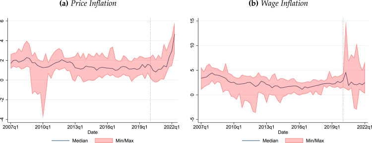
Before presenting the empirical strategy of our paper, we set the stage by discussing the behavior of prices and wage inflation internationally over the past few decades. A glimpse of their recent behavior is provided in Fig. 1, which reports a range of inflation and wage growth readings for set of OECD countries.4 Panels (a) and (b) of Fig. 1 show that price and wage inflation in these developed economies have mostly moved together in the past decade and right up to the pandemic. The common movements in inflation among developed, and even emerging, economies in the past decade is well documented in the literature, and seem to hold irrespective of their monetary policy framework (Jordà and Nechio, 2020), as inflation increasingly become a more global phenomenon. Since mid-2020, this relative smooth comovement has waned quite a bit, particularly for wages.
Fig. 1.
Price and wage inflation convergence and divergence across countries. Notes: Sample: Australia, Austria, Belgium, Canada, Denmark, Finland, France, Germany, Ireland, Italy, Netherlands, Norway, Portugal, Spain, Sweden, the United Kingdom, and the United States. Inflation based on core CPI and wage inflation measured by hourly wage compensation. Shaded area corresponds to 90% interquantile range, and vertical line marks the start of Covid-19 pandemic (2020Q1). See Section 4 for additional data details.
OECD.
A variety of factors are cited as possible drivers of the most recent rise of inflation. The Covid-19 pandemic disrupted supply chains, primarily from aggressive lockdowns implemented in China initially, and worldwide later on. Moreover, the pandemic saw a shift in consumption from services—which are usually non-tradable—to goods—which usually are—at a time when goods are in short supply (di Giovanni et al., 2022). On the demand side, strong responses from governments, which included the provision of direct payments to households, expanded demand at a time when supply was constrained. Similarly, recent upward pressures on wages have been reported in several countries (e.g., Domash and Summers, 2022, Vacas-Soriano and Kostolny, 2022, Bank of Canada, 2022, European Commission, 2021). However, the remarkable feature in both panels of the figure is how much more quickly price and wage inflation has risen in these countries.
The relative convergence of inflation before the onset of the pandemic plays an important role in our empirical analysis. In difference-in-differences analysis it is important to establish whether the parallel trends assumption holds. The idea is that before the pandemic, treated and control countries should share similar trends for the inflation process. Fig. 1 seems to indicate that this is indeed the case though we provide a more formal test later.
What may explain the relative experiences in these advanced economies? While the nature of the challenges and policy responses to the pandemic were similar in many countries, their scope varied widely. Focusing on the latter, the complexity and heterogeneity of the support measures implemented in each country make it difficult to get an accurate measure of the size and impact of their programs. For example, in the U.S., in addition to direct cash transfers to households, the government also provided loans to businesses, expanded unemployment insurance funding, and paused payments on student loans, among several other measures. Of course, each of these programs will have its own multiplier effect, not just because households at different income brackets have different marginal propensities to consume, but also because some programs enter household pockets directly (such as cash transfers and unemployment insurance, for example), while other programs have more indirect effects (such as support to businesses). Moreover, the size of the support packages varied wildly. In many countries, the size of the packages was insufficient to make up for the short-falls in demand, whereas in others (such as in the U.S.), it more than made up for it.
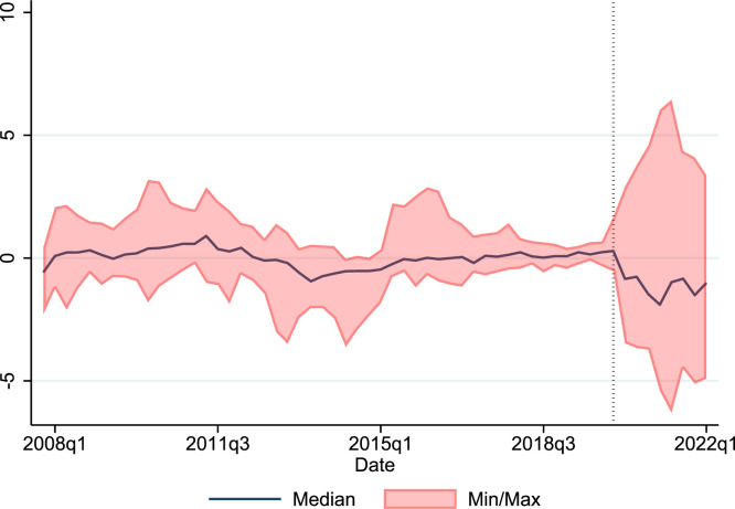
As a way to examine the effect of these programs on household incomes, we find that real disposable income per capita (RDI) offers a viable summary statistic. Fig. 2 helps visualize the effects of the programs provided across OECD economies on RDI. The figure shows that deviations of real disposable income from trend before the pandemic fluctuated in the range of , a range that has doubled to since.
Fig. 2.
The divergence of real disposable income relative to trend across countries. Notes: Sample: Australia, Austria, Belgium, Canada, Denmark, Finland, France, Germany, Ireland, Italy, Netherlands, Norway, Portugal, Spain, Sweden, the United Kingdom, and the United States. Real disposable income in deviations from trend. Shaded area corresponds to 90% interquantile range, and vertical line marks the start of Covid-19 pandemic (2020Q1). See Section 4 for additional data details.
OECD.
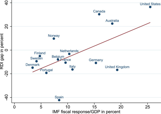
How well does the divergence in deviations of RDI from trend – the RDI gap – shown in Fig. 2 correlate with the reported fiscal effort of the countries in our sample? This is shown in Fig. 3. The figure plots the RDI gap following the pandemic (cumulative RDI gap from 2020Q1 to 2021Q4) against data from the IMF on a measure of fiscal effort as a share of GDP (total spending up to 2021 as a share of 2020 GDP). The picture shows a strong relationship between the two measures, reinforcing our interpretation that the RDI gap provides a reasonable proxy for an economic activity gap that reflects the demand shifts generated by pandemic-motivated fiscal policy.
Fig. 3.
The divergence of real disposable income relative to trend across countries. Notes: Sample: Australia, Austria, Belgium, Canada, Denmark, Finland, France, Germany, Ireland, Italy, Netherlands, Norway, Portugal, Spain, Sweden, the United Kingdom, and the United States. Real disposable income in deviations from trend. See Section 4 for additional data details.
IMF.
So why not use the IMF measures of fiscal policy shown in Fig. 3 directly? Firstly, RDI is available at a quarterly frequency, which allows us to explore the time-series properties of the effects of fiscal policies given the short sample available. Moreover, as we explained earlier, the package of measures passed by each country varied considerably and included items that resulted in direct cash transfers whereas other programs included loans and other measures that, while having similar fiscal impact, had very different effects on disposable income. Thus, we view the RDI gap as a better measure of how government actions translated into a boost of the public’s finances and thereby, a better measure of activity gap.
3. Statistical design
The previous section established two important features of the recent international experience. First, in our sample, some countries have experienced a more rapid increase in price and wage inflation than others. Second, at the same time, economies implemented a wide range of support measures during the worst of the pandemic, as Fig. 2 showed. Are these connected? Did the expansion of the public’s spending capacity push demand well beyond supply and cause prices and wages to rise? Fig. 1, Fig. 2 are not enough to provide a definitive answer. Proper statistical analysis is required.
The pandemic provides an unusual quasi-experimental setting to answer this question. All countries in our sample are affected by COVID-19 disruptions, however, different countries pursue different economic policies in response. Clearly, disruptions in supply chains and a variety of other factors affect all countries (perhaps to varying degrees). Thus, while accounting for all this heterogeneity may appear a daunting task, we think that it also offers opportunities to disentangle long-standing forces that have remained elusively documented in the literature, specially in relation to the slope of the Phillips curve—a topic that remains contentious to this date.
We tackle these issues with an identification strategy that stands on three pillars, broadly speaking: (1) a Phillips curve specification based on the real personal disposable income per capita gap () as a proxy for conditions in the demand side of the economy; (2) a difference-in-differences (DiD) approach based on sorting countries into two bins, those that pursued aggressive fiscal support (such as the U.S.)—call it the “active” group—, versus those that did not—call it the “passive” group; and (3) a local projections approach to evaluate the effects of these policies over time.
The pandemic acts as a natural exogenous event. Some countries will act as the control group, in the sense that they pursued relatively small support programs—the passive group. Other countries were considerably more aggressive – the active group – and we will think of them as the experimental or treatment group. Key to a DiD identification strategy is the assumption that the choice of fiscal response depends on factors that stayed the same before and after the pandemic. Examples may include different political traditions, access to financial markets and credibility, and so on. Moreover, we also realize that the effect of any support measure may show up on outcomes not just on impact, but over the next few periods after implementation. For these reasons and to take advantage of the unusual nature of the pandemic to achieve identification, in what follows we follow Dube et al. (2023) in formally stating our assumptions, and then in estimating the dynamic responses of interest.
3.1. Identification
We present the main assumptions by momentarily assuming treatment is binary for simplicity. When the treatment variable is continuous, it can be simply interpreted as spelling out the dose under linearity. Using the potential outcomes paradigm, we denote for the potential outcomes of our quasi-experiment with and without treatment, respectively. We think of potential outcomes as latent unobserved variables. In our analysis, , that is, price or wage inflation. Next, we will split the cross section of countries in our sample into two groups, active countries, which pursued aggressive pandemic support policies and selected by the dummy versus passive countries, which were less aggressive and for which we set . We also define the dummy variable to denote the pandemic period, and to denote the period before the pandemic. Given these two dummies, we further define as the treatment indicator.
Thus for are two latent unobserved variables. The data that we observe is a latent mixture distribution given by . The typical quantity of interest is the average treatment effect, given by . Because intervention happens only at some time , in practice, we can only estimate the average treatment effect on the treated, as is common in this literature. Moreover, since we will be interested in the dynamic effects of treatment (not just on impact but over subsequent quarters), we define our object of interest as:
| (1) |
where refers to information available when treatment is administered in country .
We depart from the DiD literature to make a more direct connection with the macroeconomic tradition of plotting impulse responses. In the DiD literature (and in Dube et al., 2023 for example), interest is in characterizing the effect of a one-time treatment, even when the outcome is exposed to several subsequent interventions, as in our case. In such settings, the information set would condition on such future treatments to sterilize their effect.
Instead, we pursue two alternative paths. First, we calculate the more traditional impulse response, which by construction incorporates the possibility that a fiscal intervention could be implemented over a number of periods. This is the interpretation of an impulse response in a typical vector autoregression (VAR), for example. Second, we will calculate multipliers, which we will define more carefully below. These are the ratio of the total effect on inflation over a period of time, divided by the total amount of fiscal interventions over that same period. The multiplier therefore looks at the total change in inflation relative to the total amount of fiscal support and thus turns out to provide an approximate measure to the one-off effect favored by the DiD tradition. Importantly, multipliers have the advantage that they are not affected by expectations mechanisms. That is, the extent to which agents anticipate future fiscal treatment will affect their current and future behavior in a way that cannot be simply sterilized by conditioning on future treatment. This is not the case with multipliers.
Two main assumptions form the basis of our identification strategy. Because the effects can be felt over several periods, we use a slightly modified version from what is traditional (see, e.g., Wooldridge, 2021 for a statement of the usual assumptions), specifically:
Assumption 1 Conditional No Anticipation —
For all i, and for all , then:
That is, since the pandemic was an exogenous event, it stands to reason that economies did not adapt in anticipation to the pandemic support that would later on be provided. We make the statement conditional on covariates observed until time (which are included in the definition of ), thereby further reinforcing the assumption.
Assumption 2 Conditional Parallel Trends —
For all i, and for all , then:
That is, treatment does not influence the evolution of the potential outcome for the control group (the “trend” in the parlance of this literature). The relative stability and similarity of price and wage inflation across economies in the lead up to the pandemic displayed in Fig. 1 (essentially the pre-trends) justify our assumption.
With these two assumptions, we can now revisit Eq. (1), repeated here for convenience:
where the second line uses the fact that when . Next, note that:
where we use the no anticipation and the parallel trends assumptions stated earlier, and the fact that when . Putting these results together, Eq. (1) can be written as:
| (2) |
which is written solely in terms of observables and thus implemented on a sample of data. Lastly, we assume that treatment effects are homogeneous, that is, we assume that the timing of when treatment is administered does not affect the treatment effect. This assumption is implicit in macroeconomics since we rely on time series regularities to identify impulse response functions. But in panel data, the cross-section dimension permits greater flexibility. That said, we will not explore this possibility in our data set since the sample available after the pandemic is much too short. The next section presents the details of how we may operationalize the local projection estimator in a DiD setting.
3.2. Local projections difference-in-differences (LP-DiD)
Building on the standard difference-in-differences approach, now let denote core CPI inflation at annual rate; let denote one-year-ahead inflation expectations (whose construction we will detail below); let denote the real personal disposable income gap (whose construction we will also detail below); let denote country-fixed effects, and time-fixed effects. Finally, define if country belongs in the active group and otherwise. Similarly, denote for the pandemic period and otherwise. Define the dummy variable . With these definitions, consider the DiD specification of a local projection:
| (3) |
In particular, the key coefficients of interest are the , which identify the effect of the RDI gap on inflation, and the , which measure the effect of shifts in expectations of inflation. Country-fixed effects, allow for heterogeneity across economies—some countries may have higher rates of inflation than others, on average, given the configuration of their economies. Similarly, time-fixed effects, help us with the evolution of the pandemic and the waves of disruptions that affected all countries at the same time, as well as controlling for global economic cycles. Importantly, the DiD approach focuses on shifts in the regression following the pandemic that happen for active countries, but not for control countries.
Specifically, note that, for example, the coefficient of Eq. (3) is not directly interpretable from an economic point of view. It is not an estimate of the slope of the Phillips curve before the pandemic. More generally, Eq. (3) should not be interpreted as a regression estimated across two regimes where one compares the slope of the Phillips curve before and after the pandemic. Rather, the slope of the Phillips curve is appropriately identified from the coefficient by exploiting variation across time and across countries. This is not obvious from a cursory glance at Eq. (3) but is an important point.
For later use in the calculation of multipliers, we use a version of Eq. (3) to estimate the response of to its own perturbations. We could use a simple autoregression, however, to work in parallel fashion to the Phillips type relations that we exploit for prices and wages (as we show in a moment), we will also estimate:
| (4) |
The coefficient of interest will be , which will collect the dynamic properties of how fiscal support measures were implemented in active countries.
Relatedly, the expression for wages takes on a similar format. Here the literature is less settled (e.g, Galí and Gambetti, 2020, Del Negro et al., 2020, Galí, 2011, and Sbordone, 2006). The specification that we will adopt here closely follows the one in Galí (2011). More specifically, let denote a measure of wage inflation (we discuss the specific measures of labor compensation below), and and as defined before. Eq. (5) poses that wages are determined by a hybrid version of a wage Phillips curve such that:
| (5) |
Several observations deserve comment. First, as with the inflation equation, country- and time-fixed effects allow us to control for substantial unobserved heterogeneity. Second, we include an inflation-expectations term to capture the idea that when nominal wages are negotiated, inflation is taken into account. Third, we leave the hybrid dynamics of these models unrestricted. We also leave the treatment effect coefficients unrestricted. Fourth, the coefficients of interest are , which are an estimate of the average treatment effect on the treated introduced in Eq. (1), . Note that these coefficient are interacted with , the gap variable, so that countries with programs of different magnitudes are properly accommodated (obviously, this works since we are working with a linear setting). In addition, we will be interested in the coefficients , which measure the effect of inflation expectations on wages and will allow us to investigate the spillover of inflation on to wages. Fifth, we also allow the coefficients on expected and past inflation to possibly vary in the active group in the pandemic period. Finally, when estimating Eqs. (3) and (5), standard errors are clustered around countries to allow for non-parametric unstructured time series features in the covariance matrix of the residuals.
We conclude this section with a brief discussion of multipliers. Because fiscal support programs were implemented over a period of time, it is natural to ask how the totality of the fiscal impetus is felt on price and wage inflation. Thus, consider the following definition, which can be found in, e.g., Mountford and Uhlig, 2009, Ramey, 2016 and Ramey and Zubairy (2018):
| (6) |
and the wage multiplier can be defined similarly. Note also that the ratio of to is also of interest as it compares the total response of inflation to the total response of wages. In the analysis, we will report estimates for all three of these quantities.
4. The data
Before discussing the sources of the data used in the analysis in detail, it is worth discussing how we construct the main variables in our analysis. Specifically:
Construction of: For all countries but Australia, we rely on one-year-ahead mean inflation projections from Consensus Economics.5 For Australia, we construct one-period-ahead inflation expectations by predicting future CPI from historical inflation data as in Hamilton et al. (2016). More specifically, using rolling windows of 20 years of quarterly data, we estimate:
| (7) |
and obtain .
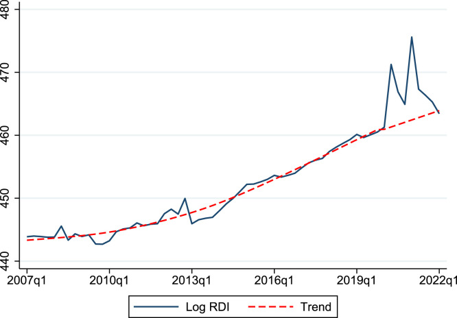
Construction of: we use the Hodrick–Prescott (HP) filter with parameter on data for the log of the real personal disposable income (RDI) index up to the start of the pandemic (2019Q4). In order to avoid over-smoothing the pandemic period (since the HP-filter would want to adjust the trend toward the boom in RDI during that period, and hence, minimize the gap), we compute a linear trend using data on log RDI from 2014 to 2019 and then use that trend from 2020 to the end of the sample. As an example of how this procedure works in practice, consider the U.S., displayed in Fig. 4. The figure shows that the HP trend is nearly linear in the years leading to the pandemic. Thus, by taking the log transformation, can be read as the approximate percent deviation from trend.6 Finally, we take a four-quarter rolling average (one year) of this gap since a boost in income does not immediately turn into increased consumption, but rather it can get smoothed over (in our case, we assume that over one year).
Fig. 4.
Calculating the U.S. RDI gap. Notes: The figure reports log RDI for the U.S. and its trend. HP filter used until 2019. Linear extrapolation from then to the end of the sample. See text.
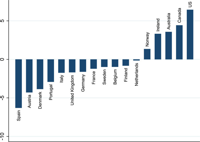
Our list of active countries, i.e., those for which , includes Australia, Canada, Ireland, Norway, and the United States. The list of passive countries, i.e., those for which , include Austria, Belgium, Denmark, Finland, France, Germany, Italy, Ireland, Netherlands, Portugal, Spain, Sweden, and the United Kingdom. The dividing line is based on whether the cumulative RDI gap was positive by 2021Q2. We choose that quarter as our benchmark as it closely marked the end of the passage of most fiscal packages. Fig. 5 depicts RDI gaps by country at that date. We experimented with alternative categorizations of countries into active and passive, which did not materially change our results.7
Fig. 5.
RDI gaps by 2021Q2. Notes: The figure reports RDI gaps by country as of 2021Q2. Countries with a positive gap implemented “active” fiscal policies, while countries with a negative gap implemented “passive” policies. See text.
We obtain cross-country data on real household gross disposable income per capita from the OECD’s “Household Dashboard: cross-country comparisons”. Our sample includes quarterly data from 2007Q1 to 2021Q4 for Australia, Austria, Belgium, Canada, Denmark, Finland, France, Germany, Ireland, Italy, Netherlands, Norway, Portugal, Spain, Sweden, the United Kingdom, and the United States.
For our estimation of Eq. (3), we rely on core CPI (Consumer Price Inflation) indices to measure inflation stripped from the effect of food and energy prices, which tend to be volatile. For our estimation of Eq. (5), we rely on headline inflation instead, which is more likely to matter for households when negotiating wage contracts than core inflation. We consider variations of these specifications in our robustness exercises. All inflation series are also sourced from OECD.
Finally, we collect data on private sector hourly wage compensation from OECD for all countries in our sample, except for Australia, Canada, Ireland and Norway. For Australia, we rely on total hourly rates (excluding bonuses) from the Australian Bureau of Statistics. For Canada, we rely on average weekly hourly earnings for all employees from Statistics Canada. For Ireland, we rely on average earnings from the National Statistical Office. And for Norway, we rely on the labor cost index for all employees from Statistics Norway.
5. Revisiting the Phillips curve mechanism
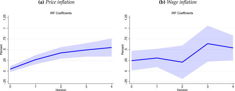
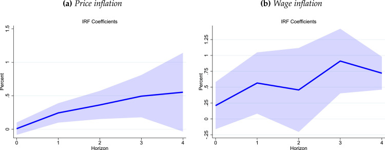
This section contains our main results. We report the dynamic response of inflation and wages to shifts in the RDI gap based on our estimates of Eqs. (3), (5).8 Fig. 6 presents the main results from estimating Eqs. (3) and (5). Panel (a) reports estimates of the activity gap coefficient for price inflation while Panel (b) reports the effects on wage inflation based on the coefficient . That is, these are the local projection estimates of the effect of changes in the activity gap from the LP-DiD procedure in Eqs. (3), (5), respectively.
Fig. 6.
The average response of price and wage inflation to pandemic support. Notes: The solid blue line reports results from the estimation of Eqs. (3), (5). The shaded area corresponds to 90% confidence bands.
The way to interpret these impulse responses is as follows. Take an increase in the activity gap of, say, 5% (this was larger in the U.S., but smaller in other countries). Then, all else equal, Panel (a) implies that this has the effect of raising inflation by about 0.1 percentage point (pp) on impact, percentage points (pps) after one quarter, over pps after two quarters, and peaking at nearly pps after quarters. The error bands displayed (90% confidence level) suggest that these effects are estimated with moderate uncertainty though they appear to be statistically different from zero and economically large.
Panel (b) of Fig. 6 displays the impulse response of the effect of the gap in economic activity (measured with RDI per capita) on wage inflation, as described in Eq. (5). Compared to the effects on price inflation, Panel (b) suggests that the effects of RDI are stronger on impact, peak a little earlier, and reach about the same level as the price inflation impulse response at the 4 quarter mark. Like the response of prices, the response of wages appears to be mostly statistically different from zero and economically large.
The effects of a boost to demand measured by a widening of the real disposable income gap with respect to trend seem large. But like any impulse response study, these impulse responses factor the likelihood of subsequent shifts in the gap. This tends to make their effect look bigger than it is. One way to address this is by calculating multipliers, which we introduced in Section 3.2, Eq. (6). As discussed there, the multiplier looks at all the changes in the RDI gap over a number of quarters and not just the gap on impact.
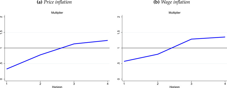
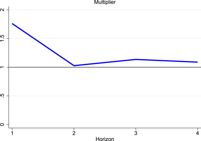
Hence, Fig. 7 reports the price and wage inflation multipliers. There are two features worth noting immediately. First is that the magnitudes are considerably smaller, as it should be. Relative to the overall increase in real disposable income, the total increase in price and wage inflation is more moderate, hovering about 1:1 at the year mark ( quarters). That is, if over a quarter period, the RDI gap increases by pp then inflation will be expected to increase by pp. Second, the price and inflation multipliers are quite similar to one another. This was perhaps not quite as evident from the impulse response figures. Since the multipliers for price and wage inflation use the same impulse response of RDI to itself in the denominator, we can take the ratio of multipliers to display a sort of price-to-wage multiplier. This is shown in Fig. 8. As expected, the figure shows that inflation is a bit quicker to respond than wages, but eventually the multiplier ratio settles around one.
Fig. 7.
The multiplier effect of pandemic support. Notes: The solid blue line is based on Fig. 7 and on Fig. 6 in addition to the impulse response of RDI gap to itself.
Fig. 8.
The inflation–wage multiplier ratio. Notes: This figure is based on the ratio of the multiplier for price inflation divided by the multiplier for wage inflation as shown in Fig. 7, See text.
What are the economic implications of our analysis? Our goal was to explore the strength of the Phillips mechanism in light of the recent pick-up in inflation. Our results suggests that this mechanism is quite important and we have provided a way to quantify how important using state-of-the art methods.
Our approach has many strengths. First, by using international data, we are able to boost the power of our conclusions. Second, our identification approach is an important departure from those used in existing studies and therefore provides a complementary way to analyze this problem. Third, our results can be used to study how important recent fiscal policy actions have been in contributing to current inflation. We will illustrate this shortly using the U.S. as an example.
However, we should also recognize the weaknesses of our approach. Since we rely on the pandemic, we cannot explore asymmetries. Should we expect the effect on inflation from fiscal restraint to be of a similar magnitude? We cannot tell. We are also limited by the particular historical episode that we have lived through during which monetary policy was specially accommodating almost everywhere. However, recent research by Cloyne et al. (2023) suggests that the fiscal multiplier depends critically on the stance of monetary policy. Thus, we cannot speak about the strength of the Phillips mechanism when monetary policy is more or less accommodating.
6. The feedback of inflation to wages
The previous section showed that the unprecedented direct fiscal support provided in during the pandemic had a significant effect on price and wage inflation since the pandemic. Moreover, inflation in many developed countries has reached levels not seen in decades. Of course, on top of the effects of the fiscal boosts, there are other reasons behind this elevated inflation readings, such as disruptions to supply chains (Santacreu and LaBelle, 2022) and, more recently, the war in Ukraine (Caldara et al., 2022). Meanwhile, the labor market upheaval brought upon by pandemic lockdowns has largely been resolved. Although the labor force has yet to fully recover, the unemployment rate sits at historically low levels and vacancy rates are at historical highs.
In such a tight labor market and elevated inflation environment, workers are likely to demand to be compensated to retain their purchasing power and have implications for how wages are set. When negotiating contracts, workers may demand higher compensation to make up for the loss of purchasing power already experienced and may want to compensate for the loss they expect to have in the future. In an environment with elevated inflation, even when longer-term inflation expectations remain well anchored and workers expect inflation to be eventually brought down to heel, their shorter-term views may become more relevant for wage setting (Glick et al., 2022).
The question that we ask in this section is a modest one. We investigate the pass-through of inflation into wages by assessing whether wage setting dynamics have changed since the pandemic. To answer this question, we once again depart from Galí (2011), which derives the wage Phillips curve by assuming that wages are set as a function of average inflation over the previous four quarters, steady-state inflation, and productivity. We modify this specification in two ways. First, we replace steady-state price inflation with inflation expectations. Next, since changes in productivity are not measured directly, we rely on time fixed effects to capture these changes. The resulting wage Phillips curve is such that wage inflation is a function of lagged wage inflation, past and expectations of price inflation, and the unemployment gap (the unemployment rate minus the natural rate).
More specifically, let refer to annual nominal wage inflation as before and define the average of annual price inflation over the previous four quarters as . Denote one-year-ahead inflation expectations as , and as deviation of the unemployment rate from its natural rate. In addition, let refer to country fixed effects, and to time fixed effects. Finally, let if , otherwise; if , otherwise. We omit and since labor markets behaved quite erratically in the early stages of the pandemic. Including these data points did not materially change our results. We estimate:
| (8) |
It is important to note the difference between this specification and the analysis we presented earlier based on DiD identification. Unlike Eq. (3), Eq. (8) is simply measuring the sensitivity of wages to headline inflation before and after the pandemic by controlling for other factors generally thought to affect the wage setting mechanism. That is, we do not claim here that, for example, and can be interpreted causally.
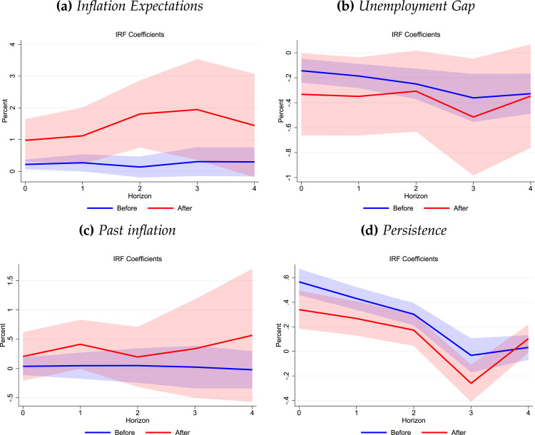
The results from estimating Eq. (8) are presented in Table 1. The table shows that before the pandemic, the pass-through of past price inflation to wage inflation is essentially zero, while inflation expectations have a coefficient of 0.18. Both are not statistically different from zero. Moreover, the unemployment gap has the correct sign and is statistically significant though, again, these are not structurally interpretable in our setup. Since the pandemic, we see an important shift in the pass-through of inflation expectations. Its coefficient increases to 0.96 (statistically significant), essentially a 1 to 1 pass-through. In addition, with the pandemic, wages exhibit somewhat lower persistence, from 0.55 to 0.34, as would be expected when price inflation is not stable and feeds more directly into wages. Finally, the coefficient on past inflation is 0.22, though still statistically no different from zero, and the coefficient on unemployment gap still has the correct sign, but its effect fades somewhat.9
Table 1.
Nominal wage setting estimation results. Eq. (8).
| Dependent variable nominal wages: | Pre-pandemic () | Post-pandemic () | |
|---|---|---|---|
| Unemployment gap: | −0.17** | −0.35 | |
| (0.07) | (0.20) | ||
| Lagged nominal wages: | 0.55*** | 0.34*** | |
| (0.07) | (0.09) | ||
| Inflation expectations: | 0.18 | 0.96** | |
| (0.14) | (0.42) | ||
| Past inflation: | 0.05 | 0.22 | |
| (0.09) | (0.25) | ||
| N. observations: | 866 | ||
| 0.48 | |||
Notes: Standard errors (in parentheses) are clustered by country. Regression includes time and fixed effects. See text.
Eq. (8) provides a static snapshot of the wage Phillips curve. To get a better sense of how the dynamics of this equation evolve over time across the two samples, Fig. 9 shows the responses calculated using local projections.10 Several features stand out. Panel (a) is the more striking. It shows a considerable difference between the role of inflation expectations across the two time samples. After the pandemic, these have clearly become quite important. Panel (b) suggests that the role of the unemployment gap is not substantially different from the economic and statistical senses. Panel (c) shows that past inflation is playing a slightly more important role since the pandemic, though its effects are imprecisely measured. Panel (d) suggests a decline in the persistence of wage inflation. Overall, these results point to an increased role for inflation expectations in explaining the dynamics of wage inflation since the pandemic.
Fig. 9.
The dynamics of the Phillips curve before and after the pandemic. Notes: Impulse responses based on Eq. (8). Before is with sample up to 2019Q4; After is with sample beginning in 2020Q3. See text.
7. Inflation and wage growth in the U.S. since the pandemic
In this section we take our empirical findings to the data to analyze their implications to recent dynamics of U.S. price and wage inflation.
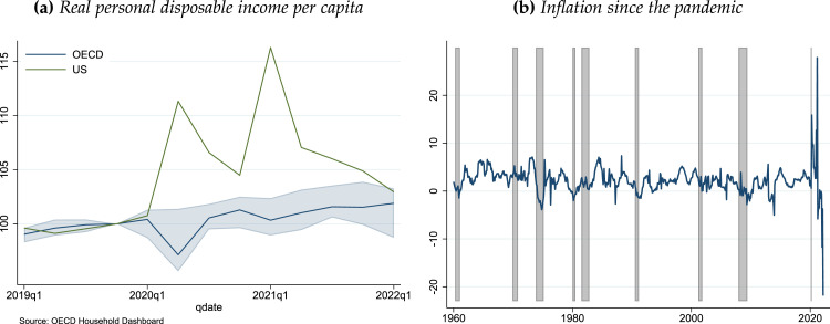
In response to the pandemic, the U.S. implemented several policies to counterbalance the effects of the pandemic. More specifically, it introduced unprecedented fiscal and monetary policy responses to provide rapid economic relief. The Coronavirus Aid, Relief, and Economic Security (CARES) Act was signed into law in March 2020 and the American Rescue Plan (ARP) Act of 2021, signed about a year later. Both Acts resulted in an unprecedented injection of direct assistance with a relatively short duration. Panel (a) of Fig. 10 provides a nice contrast between the effects of the programs provided in the U.S. versus those implemented in other OECD economies on RDI. Moreover, to put in context the magnitude of these programs relative to the post-WW2 experience in the U.S., panel (b) of Fig. 10 shows the percentage change in RDI with respect to the previous year.
Fig. 10.
The generous and unprecedented support provided by the U.S. during the pandemic. Notes: Bureau of Economic Analysis. See Section 4 for additional details.
OECD and U.S.
These panels highlight the unusual nature of the programs implemented in the U.S., whether cast against other countries, or whether compared to its own historical experience. These programs place the U.S. among the “active” countries in our sample, as detailed on Section 3.2 and illustrated in Fig. 5.
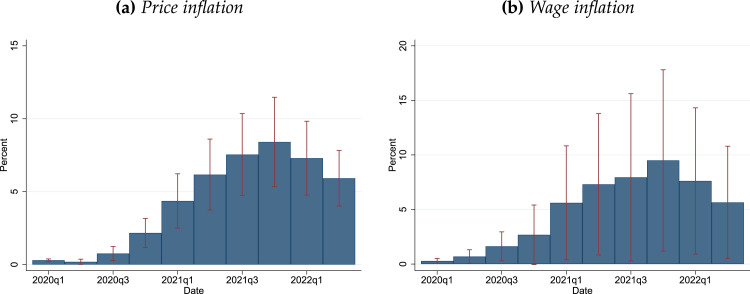
Using the estimates from Section 5 we can construct an estimate of the contribution of the Coronavirus Aid, Relief, and Economic Security (CARES) Act and the American Rescue Plan (ARP) Act to inflation in prices and wages. The CARES Act was passed into law on March 27, 2020 at the tune of $2.2 trillion. The ARP Act provided and additional $1.9 trillion and was passed into law March 11, 2021. Based on these numbers and estimates from Eqs. (3) and (5) we present their estimated contributions to inflation in prices and wages in Fig. 11.
Fig. 11.
The contribution of pandemic support to U.S. price and wage inflation. Notes: Contribution to price and wage inflation from the effects of pandemic stimulus in the U.S. on the RDI gap. Whisker bands are reported at the 90% confidence level. See text.
Several features of this figure deserve comment. Panel (a) shows that the contribution of the massive stimulus in the CARES and ARP Acts to price inflation peaks at the end of 2021, which approximately aligns with the peak of inflation in the U.S. (core PCE inflation, for example, peaked February 2022). And the contribution is estimated with relatively good precision. The peak effect on wages happens around the same time though the estimates are much more imprecise, as the whisker bands show. As we move into 2022, the effects of the stimulus begins to gradually recede and this seems to be also the case with observed price and wage inflation. The effects essentially evaporate by the end of 2023.
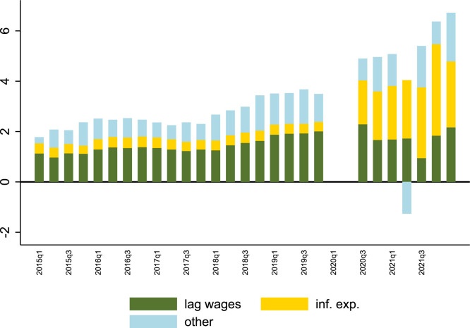
We can also reply on the estimates from Section 6 to assess the effects of inflation expectations to wage growth in the U.S. since the pandemic. As a way to visualize the contribution of each component to the evolution of wage inflation, Fig. 12 uses a stacked bar chart and shows the contributions of each regressor to wage inflation over time. The figure re-emphasizes the results reported in Table 1 in a different way, as the relative size of the bars provides some perspective that is perhaps lost when simply looking at the estimates reported in Table 1. For simplicity, we display the effects of lag wages and inflation expectations and merge all other factors in a unique item. The figure shows that since the pandemic, inflation expectations has played a much larger role than before.
Fig. 12.
Wage inflation has become more sensitive to inflation expectations. Notes: Decomposition based on estimates of Eq. (8). 2020Q1 and Q2 omitted from the sample for clarity. Lag wages refers to the lag of wage inflation; inf. exp. refers to the Consensus Forecasts of 1-year-ahead inflation; and others collects all other regressors reported in Table 1. See text.
8. Conclusion
After the pandemic, many have been surprised by the pickup in inflation. During the decade following the Great Recession, inflation had remained dormant globally. This appeared to be a challenge to the traditional Phillips mechanism and an extensive literature documented this feature, not without a great deal of controversy (see, e.g. Blanchard, 2016). However, while there are many forces common to all economies – supply chain disruptions, spikes in commodity prices due to geopolitical factors – there are growing differences in the inflation experiences around the world. In this paper we tried to find out why that is.
We use an new approach to achieve identification based on the unusual nature of the pandemic. We take this dramatic, global health event as a natural experiment. Using novel tools borrowed from the policy evaluation literature (local projections + difference-in-differences estimation), we were able to show two important features of the Phillips mechanism. First, we measure an economically and statistical Phillips mechanism via our measure of the RDI gap. Second, we show that inflation does not immediately respond to this gap. Rather it takes a few quarters. These are two important observations in the way we should think about the Phillips curve.
Credible central banks usually keep inflation expectations stable. However, the recent pick-up in inflation, at least in the short- to medium-run, means that expectations have been revised upward. Thus, in thinking how inflation may spillover into wages, we proposed a similar Phillips mechanism for wages. Wages respond to the activity gap, if anything, perhaps more strongly than prices. This is not surprising as firms have other margins over which they can adjust prices. However, we also find that wages respond to inflation expectations, though the dynamics are much slower going, as one would expect. Since the response of expectations (up to this point) has been relatively slow, the effects on wages have been relatively more modest.
What lessons should policymakers take from this research? First, we provide strong evidence that the Phillips mechanism is alive and well. A demand–supply imbalance inevitably results in inflation. Second, credibility moderates revisions of inflation expectations and this is a helpful factor in controlling price and wage inflation. Of course, maintaining this credibility requires keeping inflation at bay. The more inflation continues to grow, the more expectations will drift, and the larger the effect on price and wage inflation. Should this dynamic linger, one risks the makings of an inflation-wage spiral.
Footnotes
We are thankful for great comments from Evi Pappa, Michele Lenza, and participants of the conference “The COVID-shock and the new macroeconomic landscape: taking stock and looking ahead,” held at the European Commission in Brussels, October 6-7, 2022. Anonymous referees helped improve the paper. Celeste Liu and Fabián Rivera-Reyes provided excellent research assistance. The views expressed in this paper are the sole responsibility of the authors and do not necessarily reflect the views of the Federal Reserve Bank of San Francisco or the Federal Reserve System.
For example, the U.S. signed the Coronavirus Aid, Relief, and Economic Security (CARES) Act into law in March 2020 which among other measures, included payments up to $1,200 per eligible individuals. The American Rescue Plan Act passed in March 2021, raised that amount to $1,400.
The program is known as Kurzarbeit in Germany.
As of writing this paper, core inflation in the U.S., U.K., and Canada is running around 2 percentage points higher than in the euro area.
OECD countries included in the analysis are Australia, Austria, Belgium, Canada, Denmark, Finland, France, Germany, Ireland, Italy, Netherlands, Norway, Portugal, Spain, Sweden, the United Kingdom, and the United States.
Consensus Forecasts are published by Consensus Economics. The publication surveys over 250 financial and economic forecasters on their projections for a range of variables, including GDP growth, inflation, interest rates and exchange rates. We take mean quarterly one-year-ahead “consumer price” inflation projections.
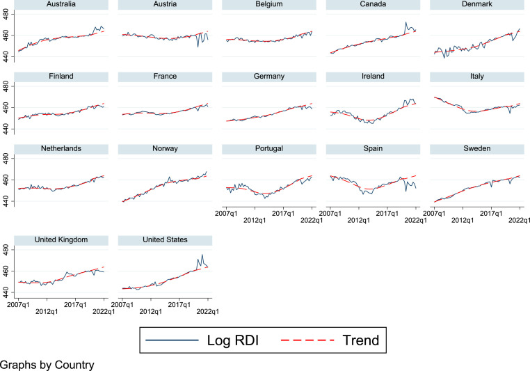
The Appendix Fig. A.1 shows RDI and its trend for all countries in our sample.
In particular, we redid our exercise after dropping Norway, Netherlands, Finland, and Belgium from our sample. These are the countries where the RDI gap is closest to zero in Fig. 5. Results are qualitatively unchanged and reported on Fig. A.2. We also considered, alternatively, setting the threshold such that “active” countries are those in which the (four-quarter rolling average) cumulative RDI gap exceeded 1% (as in Jordà et al., 2022). The set of countries in the active and passive groups are exactly the same as in our benchmark exercise.
In our benchmark results, we exclude from our sample the first two quarters of 2020 since labor markets behaved quite erratically in the early stages of the pandemic. Including these data points did not materially change our results.
Galí (2011) estimates a similar specification in Table 2 of his paper. He includes 2 lags of the unemployment gap whose coefficients add up to −0.096, which are close to our findings. Similarly, his estimate of the parameter on the lagged wage inflation average is 0.642, close to our estimate of 0.55 in the pre-pandemic period, and not far from 0.34 in the post-pandemic period given the uncertainty of this estimate. Of course, his sample and specification are quite different from ours, hence, it is reassuring that we find similar results for the pre-pandemic sample. He relies on U.S. data only and his sample runs from to .
The left-hand side is wage inflation at some point in the future.
Supplementary material related to this article can be found online at https://doi.org/10.1016/j.euroecorev.2023.104474.
Appendix A.
Fig. A.1.
RDI gap by country. Notes: The figure reports log RDI and its trend for each country in our sample. HP filter used until 2019. Linear extrapolation from then to the end of the sample. See text.
Fig. A.2.
The average response of price and wage inflation to pandemic support. Notes: The solid blue line reports results from the estimation of Eqs. (3), (5). The shaded area corresponds to 90% confidence bands. The sample excludes Norway, Netherlands, Finland, and Belgium, whise RDI gap is nearly zero by 2021Q2.
Appendix B. Supplementary data
The following is the Supplementary material related to this article.
.
Data availability
The authors do not have permission to share data.
References
- Bank of Canada . Bank of Canada; 2022. Business Outlook Survey — First Quarter of 2022: Technical Report 19.1. [Google Scholar]
- Blanchard O. The Phillips Curve: Back to the’60s?Am. Econ. Rev. 2016;106(5):31–34. [Google Scholar]
- Brinner R.E. The Death of the Phillips Curve ReconsideredQ. J. Econ. 1977;91(3):389–418. [Google Scholar]
- Caldara D., Conlisk S., Iacoviello M., Penn M. The Effect of the War in Ukraine on Global Activity and Inflation. Board of Governors of the Federal Reserve System; Washington: 2022. (FEDS Notes). [Google Scholar]
- Cameron A.C., Trivedi P.K. Cambridge University Press; 2005. Microeconometrics: Methods and Applications. [Google Scholar]
- Cloyne J.S., Jordà Ò., Taylor A.M. National Bureau of Economic Research; 2023. State-dependent local projections: Understanding impulse response heterogeneity: Technical Report 30971. [Google Scholar]
- Del Negro M., Lenza M., Primiceri G.E., Tambalotti A. What’s Up with the Phillips Curve?Brook. Pap. Econ. Act. 2020:301–357. [Google Scholar]
- di Giovanni J., Kalemli-Özcan S., Silva A., Yildirim M.A. National Bureau of Economic Research; 2022. Global Supply Chain Pressures, International Trade, and Inflation: Working Paper 30240. [Google Scholar]
- Domash A., Summers L.H. National Bureau of Economic Research; 2022. How Tight are U.S. Labor Markets?: Working Paper 29739. [Google Scholar]
- Dube A., Girardi D., Jordà Ò., Taylor A.M. National Bureau of Economic Research; 2023. A Local Projections Approach to Difference-in-Differences Event Studies: Technical Report 31184. [Google Scholar]
- European Commission A. European Commission; 2021. Labour Market and Wage Developments in Europe: Annual Review. [Google Scholar]
- Galí J. The Return of The Wage Phillips CurveJ. Eur. Econ. Assoc. 2011;9(3):436–461. [Google Scholar]
- Galí J., Gambetti L. Has the U.S. Wage Phillips Curve Flattened? A Semi-structural ExplorationSer. Banca Cent. Anál. Polít. Econ. 2020;(27) [Google Scholar]
- Ghanem D., Sant’Anna P.H., Wüthrich K. Selection and Parallel Trends. 2022. arXiv preprint arXiv:2203.09001. [Google Scholar]
- Glick R., Leduc S., Pepper M. Will Workers Demand Cost-of-Living Adjustments?FRBSF Econ. Lett. 2022;2022–21 [Google Scholar]
- Hamilton J.D., Harris E.S., Hatzius J., West K.D. The Equilibrium Real Funds Rate: Past, Present, and FutureIMF Econ. Rev. 2016;64(4):660–707. [Google Scholar]
- Jordà Ò. Estimation and Inference of Impulse Responses by Local ProjectionsAm. Econ. Rev. 2005;95(1):161–182. [Google Scholar]
- Jordà Ò., Liu C., Nechio F., Rivera-Reyes F. Why Is U.S. Inflation Higher than in Other Countries?FRBSF Econ. Lett. 2022;2022(07):1–06. [Google Scholar]
- Jordà Ò., Nechio F. Inflation GloballySer. Banca Cent. Anál. Polít. Econ. 2020;(27) [Google Scholar]
- McLeay M., Tenreyro S. Optimal Inflation and the Identification of the Phillips CurveNBER Macroecon. Annu. 2020;34(1):199–255. [Google Scholar]
- Mountford A., Uhlig H. What are the Effects of Fiscal Policy Shocks?J. Appl. Econom. 2009;24(6):960–992. [Google Scholar]
- Phillips A.W. The Relation between Unemployment and the Rate of Change of Money Wage Rates in the United Kingdom, 1861-1957Economica. 1958;25(100):283–299. [Google Scholar]
- Ramey V.A. Macroeconomic Shocks and their PropagationHandb. Macroecon. 2016;2:71–162. [Google Scholar]
- Ramey V.A., Zubairy S. Government Spending Multipliers in Good Times and in Bad: Evidence from US Historical DataJ. Polit. Econ. 2018;126(2):850–901. [Google Scholar]
- Ratner D., Sim J.W. Board of Governors of the Federal Reserve System; 2022. Who Killed the Phillips Curve? A Murder Mystery: Finance and Economics Discussion Series 2022–028. [Google Scholar]
- Rubin D.B. Estimating Causal Effects of Treatments in Randomized and Nonrandomized StudiesJ. Educ. Psychol. 1974;66(5):688. [Google Scholar]
- Santacreu A.M., LaBelle J. Global Supply Chain Disruptions and Inflation During the COVID-19 PandemicFed. Reserv. Bank St. Louis Rev. 2022;Second Quarter [Google Scholar]
- Sbordone A.M. U.S. Wage and Price Dynamics: A Limited-Information ApproachInt. J. Cent. Bank. 2006;2(3) [Google Scholar]
- Vacas-Soriano C., Kostolny J. European Foundation for the Improvement of Living and Working Conditions; 2022. Minimum Wages in 2022: Bigger Hikes this Time Around: Technical Report EF22041. [Google Scholar]
- Wooldridge J.M. MIT Press; 2010. Econometric Analysis of Cross Section and Panel Data. [Google Scholar]
- Wooldridge J. Two-way Fixed Effects, the Two-Way Mundlak Regression, and Difference-in-Differences Estimators. 2021. Available at SSRN 3906345. [Google Scholar]
Associated Data
This section collects any data citations, data availability statements, or supplementary materials included in this article.
Supplementary Materials
.
Data Availability Statement
The authors do not have permission to share data.


