Stationary distribution and density function analysis of SVIS epidemic model with saturated incidence and vaccination under stochastic environments

Abstract

In this article, we study the dynamical properties of susceptible-vaccinated-infected-susceptible (SVIS) epidemic system with saturated incidence rate and vaccination strategies. By constructing the suitable Lyapunov function, we examine the existence and uniqueness of the stochastic system. With the help of Khas’minskii theory, we set up a critical value $R_s^{\ast }$ with respect to the basic reproduction number $R^{\ast }$ of the deterministic system. A unique ergodic stationary distribution is investigated under the condition of $R_s^{\ast }>1$. In the epidemiological study, the ergodic stationary distribution represents that the disease will persist for long-term behavior. We focus for developing the general three-dimensional Fokker–Planck equation using appropriate solving theories. Around the quasi-endemic equilibrium, the probability density function of the stochastic system is analyzed which is the main theme of our study. Under $R_s^{\ast }>1$, both the existence of ergodic stationary distribution and density function can elicit all the dynamical behavior of the disease persistence. The condition of disease extinction of the system is derived. For supporting theoretical study, we discuss the numerical results and the sensitivities of the biological parameters. Results and conclusions are highlighted.

Introduction

Recently, global social economics and human health are greatly affected by the infectious disease. The awareness has been increased for preventing and to control the world-wide spreading of COVID-19. Mathematical model is one of the most important tools to describe the behavior of the epidemic in epidemiology. Kermack and Mckendric (1927) investigated a susceptible-infected-susceptible (SIS) model and discussed its dynamical properties. The transmissions of various epidemics (Liu et al. 2008; Li et al. 2017, 2001; Jerubet and Kimathi 2019; Hove-Musekwa and Nyabadza 2009; Iwami et al. 2007; Cai and Wu 2009; Vincenzo and Gabriella 1978; Carter et al. 2020; Mahato et al. 2021; Das et al. 2021) were developed with realistic ordinary differential equation. (Kuniya and Wang 2018) established a susceptible-infected-recovered (SIR) epidemic model. They studied the existence of the global stability of disease-free equilibrium for basic reproduction number $R_0<1$ and investigated the uniform persistence of the system under $R_0>1.$ (Naik et al. 2020a) formulated a SIR epidemic model with Crowley–Martin incidence rate and Holling type–II treatment. With the help of La-Salle invariance principle and the Lyapunov function, they examined the existence and stability of both equilibrium points. A nonlinear fractional infectious disease model in HIV transmission was discussed by Naik et al. (2020b). A SIRS epidemic model with mixed vaccination strategies was established by Gao et al. (2011). They added the seasonal variability on infection in their study. A SVIR (Susceptible-Vaccinated-Infected-Recovered) epidemic model was studied by Liu et al. (2008). They discussed the vaccine strategies for controlling the disease. Xing and Li (2021) established a SVIR epidemic model with relapse and investigated the persistence of the epidemic. Lee and Lao (2018) described an epidemic model with bilinear incidence rate and investigated the transmission dynamics of the disease.

Environmental variations (Liu et al. 2018; Cai and Kang 2015) may perturb the travel of population, design of control strategies. Many researchers formulated the stochastic differential equation for epidemic and analyzed their dynamical behavior. A stochastic SIS epidemic model with vaccination was studied by Zhao and Jiang (2014). The theory of extinction and persist in mean of the epidemic was investigated in their work. In Caraballo et al. (2020), Carballo et al. formulated a stochastic SIRS epidemic model and discussed the condition of stationary distribution. The existence of ergodic stationary distribution and the probability density function of the SVIS epidemic model were studied by Zhou et al. (2020). Zhou et al. (2021) solved the general three-dimensional Fokker–Planck equation. The existence of stationary distribution and ergodicity of the system has been discussed. They have studied the impact of random noises on the disease extinction.

Concentration in the vaccination on infected individuals and random oscillation, the main theme of our study is to improve SIVS epidemic model in stochastic nature with vaccination strategies. The disease which will be persistent depends on the corresponding basic reproduction number of the system. There is no positive equilibrium exists in the stochastic system for the environmental fluctuation. So, the stochastic permanence of the epidemic can be greatly affected by the existence of a stationary distribution and the properties of ergodicity. For controlling the outbreak of epidemic, we must need for statistical data of the disease in our real life. For difficulties to solve the higher-order Fokker–Planck equations, we have analyzed the probability density function. In this work, some studies of probability density function of stationary distribution are discussed. For this, we focus for three points.

• (i)Comprise stochastic threshold $R_S^{\ast }$ with respect to the basic reproduction number $R^{\ast }.$
• (ii)Look into the persistence of the disease of stochastic SVIS system under the condition of $R_S^{\ast }>1.$
• (iii)Discuss the numerical simulation and the sensitivities of the ecological parameters of the system get a clear view of our study.

This work is represented as follows: Sect. "Model calibration and dynamical behavior:" presents model formulation and necessary notation for the model. Sect. "Persistence and extinction of the system" introduces the persistence and the extinction of the stochastic system. The ergodic stationary distribution under $R_S^{\ast }>1$ is investigated in the subsection of 3. Sect. "Numerical results:" shows some numerical results and Sect. "Sensitivities of the parameters:" represents the sensitivities of the parameters. Finally, results are discussed and conclusions are drawn in Sect. "Discussion of results."

Model calibration and dynamical behavior

In this section, the deterministic and stochastic SVIS epidemic models are developed after considering some suitable conditions.

Deterministic SVIS epidemic system

Suppose, $N(t)$ is the total investigated population. This population is divided into susceptible $S\left(t\right),$ vaccinated $V\left(t\right),$ infected $I(t)$ populations at any instant $t.$ In this study, the susceptible individuals obey the rule of logistic growth model which is the growth process of species in natural way (Jiang et al. 2007; Arino et al. 2006; Xu et al. 2015). We formulate a deterministic SVIS epidemic system (Zhou et al. 2020, 2021) with saturated incidence and vaccination strategies, which is given as

$$\frac{dS\left(t\right)}{\mathit{dt}}=pS\left(t\right)\left(1-\frac{S\left(t\right)}{q}\right)-\frac{\lambda S\left(t\right)I\left(t\right)}{1+k_{1}I\left(t\right)}-\psi S\left(t\right)-{\alpha }_{1}S\left(t\right)+{\beta }_{2}I\left(t\right)+{\beta }_{1}V\left(t\right)$$

$$\frac{dV\left(t\right)}{\mathit{dt}}={\alpha }_{1}S\left(t\right)-\left({\beta }_1+\psi \right)V\left(t\right)$$

$$\frac{dI\left(t\right)}{\mathit{dt}}=\frac{\lambda S\left(t\right)I\left(t\right)}{1+k_{1}I\left(t\right)}-\left(\psi +{\alpha }_2+{\beta }_2\right)I\left(t\right)$$ 1

where $p,q,\lambda ,k_1,\psi ,{\alpha }_1,{\beta }_2,{\beta }_1$ and ${\alpha }_2$ are all positive constants. The parameter $p$ is the intrinsic growth rate of susceptible individuals, and $q$ depicts the carrying capacity of $S\left(t\right).$ The term $\frac{\lambda S\left(t\right)I\left(t\right)}{1+k_{1}I\left(t\right)}$ is more sensitive than the bilinear incidence rate in epidemiological study (Zhu et al. 2020; Xu et al. 2016; Batabyal and Batabyal 2021; Chong et al. 2014). Here, $\lambda$ denotes the disease transmission rate between susceptible and infected individuals, and $k_1$ is the half-saturation constant. The parameters $\psi$ and ${\alpha }_1$ represent the natural mortality rate of all individuals and vaccination rate of susceptible individuals, respectively. The disease-related death rate of the infected individuals is represented by ${\alpha }_2$. The immunity loss coefficient of the vaccinated individuals and the recovery rate of the infected individuals are depicted by the parameters ${\beta }_1$ and ${\beta }_2$, respectively. Ecological description of the parameters and its units are shown in Appendix 1.

The disease-free equilibrium point of the system is given by

$$E^{\#}=\left(S^{\#},V^{\#},I^{\#}\right)=\left[\frac{q}{p}\left\{\frac{\left(p-\psi -{\alpha }_1\right)\left({\beta }_1+\psi \right)+{\beta }_1{\alpha }_1}{{\beta }_1+\psi }\right\},\frac{{\alpha }_1}{({\beta }_1+\psi )}\frac{q}{p}\left\{\frac{\left(p-\psi -{\alpha }_1\right)\left({\beta }_1+\psi \right)+{\beta }_1{\alpha }_1}{{\beta }_1+\psi }\right\},0\right].$$

Now, we compute the basic reproduction number (Driessche and Watmough 2002) of the deterministic system.

$R^{\ast }=\frac{\lambda q\left\{\left(p-\psi -{\alpha }_1\right)\left({\beta }_1+\psi \right)+{\beta }_1{\alpha }_1\right\}}{p({\beta }_1+\psi )\left(\psi +{\alpha }_2+{\beta }_2\right)}$ (see Appendix 2). Actually, the basic reproduction number $R^{\ast }$ can be defined as the number of new infections started from infective individuals at disease-free equilibrium. $R^{\ast }<1$ indicates infected population creates less than one new infected population at time of its infective situation and the disease becomes extinct. In other way, $R^{\ast }>1$ represents that each infected populations create more than one new infection, and then, the infection can spread over the population.

For the endemic equilibrium point of the system (1), we obtain.

$E^{@}=\left(S^{@},V^{@},I^{@}\right)$ and $S^{@}=\frac{({\beta }_1+\psi )V^{@}}{{\alpha }_1}$, $I^{@}=\frac{1}{\psi +{\alpha }_2}\left[\frac{({\beta }_1+\psi )}{{\alpha }_1}\left\{p\left(1-\frac{k_1}{q}\right)-\left(\psi +{\alpha }_1\right)\right\}+{\beta }_1\right]V^{@}$. where $V^{@}$ is the root of the following equation

$E_1{\left(V^{@}\right)}^2+E_2{V}^{@}+E_3=0$ and $E_1=\frac{\left(\psi +{\alpha }_2+{\beta }_2\right)p}{{\alpha }_1\left(\psi +{\alpha }_2\right)q}$, $E_2=\frac{\lambda }{\alpha ({\beta }_1+\psi )}-\frac{p\left(\psi +{\alpha }_2+{\beta }_2\right)}{{\alpha }_1\left(\psi +{\alpha }_2\right)\left({\beta }_1+\psi \right)}$,

$$E_3=\frac{\psi +{\alpha }_2+{\beta }_2}{{({\beta }_1+\psi )}^2}.$$

Stochastic SVIS epidemic system

In real life, the dynamical properties of the maximum epidemiological model are greatly influenced by random perturbation in the environments. With the help of relevant study (Cai and Kang 2015; Zhao and Jiang 2014; Khan and Khan 2018; Zhang 2017; Caraballo et al. 2020; Wang and Jiang 2019; Wang and Wang 2018; Liu et al. 2019a; Zhou et al. 2020), we consider the stochastic perturbations are directly proportional to $S\left(t\right),V\left(t\right)$, $I\left(t\right)$. Stochastic perturbations are influenced by multiplicative noises. These multiplicative noises are considered for describing the non-equilibrium systems to better understand the fluctuations which are not self-originating. So, the corresponding stochastic SVIS epidemic system with vaccination strategies is formulated by

$$dS\left(t\right)=\left[pS\left(t\right)\left(1-\frac{S\left(t\right)}{q}\right)-\frac{\lambda S\left(t\right)I\left(t\right)}{1+k_{1}I\left(t\right)}-\psi S\left(t\right)-{\alpha }_{1}S\left(t\right)+{\beta }_{2}I\left(t\right)+{\beta }_{1}V\left(t\right)\right]dt+{\tau }_{1}Sd{G}_1\left(t\right)$$

$$dV\left(t\right)=\left[{\alpha }_{1}S\left(t\right)-\left({\beta }_1+\psi \right)V\left(t\right)\right]dt+{\tau }_{2}Vd{G}_2\left(t\right)$$

$$dI\left(t\right)=\left[\frac{\lambda S\left(t\right)I\left(t\right)}{1+k_{1}I\left(t\right)}-\left(\psi +{\alpha }_2+{\beta }_2\right)I\left(t\right)\right]dt+{\tau }_{3}Id{G}_3\left(t\right)$$ 2

Here, $G_i\left(t\right)\left(i=1,2,3\right)$ are the independent standard Brownian motions and ${\tau }_i\left(i=1,2,3\right)$ are their intensities.

Existence and uniqueness

Now, we have investigated the existence and uniqueness of the solutions.

Theorem 1

The solutions $\left\{S\left(t\right),V\left(t\right),I\left(t\right)\right\}\in R_3^{+}$ of the stochastic system (2) are unique and exist in the region $R_3^{+}$ for the initial values $\left\{S\left(0\right),I\left(0\right),V\left(0\right)\right\}\in R_3^{+}.$

Proof

The coefficients of the system (2) are locally Lipschitz continuous as reported by of Mao et al. (Mao 1997). $\left\{S\left(t\right),V\left(t\right),I\left(t\right)\right\}\in R_3^{+},t\in \left(0,{\sigma }_0\right)$ is the solution of the system (2) for the initial values $\left\{S\left(0\right),I\left(0\right),V\left(0\right)\right\}\in R_3^{+}$. ${\sigma }_0$ depicts the explosion time. For proving the global solution, we must prove ${\sigma }_0=\infty$ a.s. The stopping time is satisfied the following conditions.

${\sigma }_n=\text{inf}\{0<t<{\sigma }_0:\text{min}\left\{S\left(t\right),V\left(t\right),I\left(t\right)\right\}\le \frac{1}{\delta }$ or max $\left\{S\left(t\right),V\left(t\right),I\left(t\right)\right\}\ge \delta \}$.where, $\left\{S\left(0\right),I\left(0\right),V\left(0\right)\right\}\in \left[\frac{1}{{\delta }_0},{\delta }_0\right]$ and $\delta \ge {\delta }_0.$

We also assume the set inf{Φ} = $\infty$, when $n\to \infty$ then ${\sigma }_n$ is increasing. Thus, we get ${\sigma }_{\infty }=\underset{n\to \infty }{lim}{\sigma }_n.$ If we show that ${\sigma }_{\infty }=\infty$ almost surely, then ${\sigma }_0=\infty$ almost surely. This implies that $\left\{S\left(t\right),V\left(t\right),I\left(t\right)\right\}\in R_3^{+}$ almost surely for $t\ge 0.$ When ${\sigma }_{\infty }<\infty$, then there exist two positive constants $M$ and $\epsilon$ such that $P\left\{{\sigma }_{\infty }\le M\right\}>\epsilon$. Again, we define.

$P\left\{{\sigma }_n\le M\right\}\ge \epsilon$ for any integer ${\delta }_1\ge {\delta }_0.$

Let us assume a fundamental function $\widehat{F:}{R}_3^{+}\to R$ such that $\widehat{F}\left(S,V,I\right)=\left(S-\text{In}S-1\right)+\left(V-\text{InV}-1\right)+\left(I-1-\text{In}I\right).$ As $w>0$, then $\left(w-1-\text{In}w\right)\ge 0$. Thus $\widehat{F}\left(S,V,I\right)$ is non-negative $C^2$ function.

Using It $\widehat{\text{o}}$’s formula, we obtain

$$\text{d}\widehat{F}\left(S,V,I\right)=\mathbb{L}\widehat{F}\left(S,V,I\right)\text{d}t+{\tau }_1\left(S-1\right)\text{d}{G}_1\left(t\right)+{\tau }_2\left(V-1\right)\text{d}{G}_2\left(t\right)+{\tau }_3\left(I-1\right)\text{d}{G}_3\left(t\right)$$

where $\mathbb{L}\widehat{F}\left(S,V,I\right)=\left(1-\frac{1}{S}\right)\left[pS\left(1-\frac{S}{q}\right)-\frac{\lambda SI}{1+k_{1}I}-\psi S-{\alpha }_{1}S+{\beta }_{2}I+{\beta }_{1}V\right]+\frac{{\tau }_1^2}{2}+\left(1-\frac{1}{V}\right)\left[{\alpha }_{1}S-\left({\beta }_1+\psi \right)V\right]+\frac{{\tau }_2^2}{2}+\left(1-\frac{1}{I}\right)\left[\frac{\lambda SI}{1+k_{1}I}-\left(\psi +{\alpha }_2+{\beta }_2\right)I\right]+\frac{{\tau }_3^2}{2}$

$$\le p+3\psi +{\alpha }_1+{\alpha }_2+{\beta }_1+{\beta }_2+\frac{{\tau }_1^2+{\tau }_2^2+{\tau }_3^2}{2}-p\left(1-\frac{S}{q}\right)+\frac{\lambda I}{1+k_{1}I}$$

$$\le p+3\psi +{\alpha }_1+{\alpha }_2+{\beta }_1+{\beta }_2+\frac{{\tau }_1^2+{\tau }_2^2+{\tau }_3^2}{2}\le \widehat{H}.$$

Therefore, we get. $\text{d}\widehat{F}\left(S,V,I\right)\le \widehat{H}\text{d}t+\left[{\tau }_1\left(S-1\right)\text{d}{G}_1\left(t\right)+{\tau }_2\left(V-1\right)\text{d}{G}_2\left(t\right)+{\tau }_3\left(I-1\right)\text{d}{G}_3\left(t\right)\right]$.

We integrate both sides with respect to limit runs from $0$ to ${\sigma }_n\wedge \text{M}$ and take expectation,

$$\mathbb{E}\widehat{F}\left(S\left({\sigma }_n\wedge M\right),V\left({\sigma }_n\wedge M\right),I\left({\sigma }_n\wedge \text{M}\right)\right)\le \widehat{H}\mathbb{E}\left({\sigma }_n\wedge \text{M}\right)+\widehat{F}\left(S\left(0\right),V\left(0\right),I\left(0\right)\right)\le \widehat{H}M+\widehat{F}\left(S\left(0\right),V\left(0\right),I\left(0\right)\right).$$

Let us consider ${\mathrm{\Omega }}_m=\left\{{\sigma }_n\le M\right\}$. for $m\ge m_1$., then $P\left({\mathrm{\Omega }}_m\right)\ge \epsilon .$.

For every $\eta \in {\mathrm{\Omega }}_m,$ such that $S\left({\sigma }_n,\eta \right),V\left({\sigma }_n,\eta \right),I\left({\sigma }_n,\eta \right)$ is equal to $\frac{1}{m}$ or $m.$

So, $\widehat{F}\left(S\left({\sigma }_m,\eta \right),V\left({\sigma }_m,\eta \right),I\left({\sigma }_m,\eta \right)\right)$ is not less than either $m-1-\text{ln}m$ or $\frac{1}{m}-1+\text{ln}m.$

$$\widehat{H}M+\widehat{F}\left(S\left(0\right),V\left(0\right),I\left(0\right)\right)\ge \mathbb{E}[T_{{\mathrm{\Omega }}_m}(\eta )\widehat{F}\left(S\left({\sigma }_m,\eta \right),V\left({\sigma }_m,\eta \right),I\left({\sigma }_m,\eta \right)\right)]$$

$$\ge \epsilon \left\{m-1-\text{ln},m\right\}\wedge \left\{\frac{1}{m}-1+\text{ln},m\right\}$$

Here, $T_{{\mathrm{\Omega }}_m}$ represents the indicator function of ${\mathrm{\Omega }}_m.$ Applying $m\to \infty$ both sides, that gives a contradiction

$$\infty =\widehat{H}M+\widehat{F}\left(S\left(0\right),V\left(0\right),I\left(0\right)\right)<\infty .$$

This gives us ${\sigma }_{\infty }=\infty$ a.s. Hence, the proof is completed.

Persistence and extinction of the system

In this section, we have discussed the persistence and the extinction of the system. For this purpose, we define that the stochastic reproductive ratio of the system (2) is $R_S^{\ast }=\frac{\lambda q\left\{{\alpha }_1{\beta }_1+\left({\beta }_1+\psi \right)\left(p-\psi -{\alpha }_1\right)\right\}}{\left(p+\frac{{\tau }_1^2}{2}\right)\left({\beta }_1+\psi +\frac{{\tau }_2^2}{2}\right)\left(\psi +{\alpha }_2+{\beta }_2+\frac{{\tau }_3^2}{2}\right)}$.

Stationary Distribution and ergodic property of the Stochastic System

Since the stochastic system (2) has no endemic equilibrium point, we examine the ergodic stationary distribution that represents the persistence of the disease. Now, we study some important lemma of the theory of Khas’minskii (Khas’miniskii RZ 1980).

Let us assume a stochastic differential equation

$$\text{d}Y\left(t\right)=g\left(y\right)\text{d}t+\sum _{k=1}^n{h}_k\left(y\right)\text{d}{G}_k\left(t\right)$$

where $Y\left(t\right)$ is a homogeneous Markov process in d-dimensional Euclidean space ${\gamma }_d.$ The diffusion matrix is $B\left(Y\right)=\left(b_{\mathit{ij}}\left(y\right)\right);$ and $b_{\mathit{ij}}\left(y\right)=\sum _{l=1}^n{h}_l^{\left(i\right)}\left(y\right)h_l^{\left(j\right)}\left(y\right).$

Lemma 1

Zhou et al. 2021; Khas’miniskii RZ 1980): The Markov process $Y\left(t\right)$ has a unique ergodic stationary distribution $\pi \left(.\right)$ for any bounded region $R$ with boundary $\pi$ and.

• (i)There is a non-negative integer $N$ such that $\sum _{i,j=1}^d{b}_{\mathit{ij}}\left(y\right){\kappa }_i{\kappa }_j\ge N{\left|k\right|}^2$, $y\in R,\kappa \in R^d.$
• (ii)There is a non-negative $C^2$ function $F\left(Y\left(t\right)\right)$ such that $LF\left(Y\left(t\right)\right)$ is negative for $y\in {\mathrm{\Omega }}_R\backslash R$. Then, for all $y\in R^d$ and integral function $\chi \left(.\right)$ with respect to the measure $\chi \left(.\right)$, it follows that

$P\left\{\underset{q\to \infty }{lim}\frac{1}{q}\underset{0}{\overset{q}{\int }}\chi (y\left(t\right))=\int \chi \left(y\right)\pi \left(\text{d}y\right)\right\}=1$.

Theorem 2

The stochastic system (2) has ergodic property and a unique stationary distribution $\pi \left(.\right)$ for the initial value $\left\{S\left(0\right),V\left(0\right),I\left(0\right)\right\}\in R_3^{+}$ and $R_S^{\ast }>1.$

Proof

In the previous theorem, we prove the unique global positive solution for the initial values $\left\{S\left(0\right),V\left(0\right),I\left(0\right)\right\}\in R_3^{+}.$ For proving this theorem, we only verify Lemma 1.

We choose a $C^2$ function $Z$ such that

$$Z\left(S,V,I\right)=N_0\left(S+V+I-b_1\text{ln}S-b_1{b}_2\text{ln}V-b_3\text{ln}I\right)-\text{ln}S-\text{ln}V+\left(S+V+I\right)$$

where $b_1,b_2,b_3$ all are positive constants and $N_0=\frac{p\left(1-\frac{S}{q}\right)+2\psi +{\beta }_1+{\alpha }_1+\frac{{\tau }_1^2+{\tau }_2^2}{2}+2}{3p\left(\sqrt[3]{R_S^{\ast }}-1\right)\left(1-\frac{S}{q}\right)}>0.$

From above expression, we have

$$-3N_{0}p\left(1-\frac{S}{q}\right)\left(\sqrt[3]{R_S^{\ast }}-1\right)+p\left(1-\frac{S}{q}\right)+2\psi +{\beta }_1+{\alpha }_1+\frac{{\tau }_1^2+{\tau }_2^2}{2}=-2$$

For simplification,

$$Z_1=\left(S+V+I-b_1\text{ln}S-b_1{b}_2\text{ln}V-b_3\text{ln}I\right)$$

$$Z_2=-\text{ln}S-\text{ln}V;Z_3=S+V+I$$

Using It ${\widehat{o}}^{\prime }$ s formula to $Z_1$ (see Appendix 3) we derive

$$L{Z}_1=p\left(1-\frac{S}{q}\right)-\psi \left(S+V+I\right)-{\alpha }_{2}I-b_1\left[p\left(1-\frac{S}{q}\right)-\frac{\lambda I}{1+k_{1}I}+{\beta }_2\frac{I}{S}+{\beta }_1\frac{V}{S}-\left(\psi +{\alpha }_1+\frac{{\tau }_1^2}{2}\right)\right]-b_1{b}_2\left[{\alpha }_1\frac{S}{V}-\left({\beta }_1+\psi +\frac{{\tau }_2^2}{2}\right)\right]-b_3\left[\frac{\lambda S}{1+k_{1}I}-\left(\psi +{\alpha }_2+{\beta }_2+\frac{{\tau }_3^2}{2}\right)\right]$$

$$\le p\left(1-\frac{S}{q}\right)-\left[\psi N+b_{1}p\left(1-\frac{S}{q}\right)+\frac{b_3\lambda S}{1+k_{1}I}\right]+b_1\left(\psi +{\alpha }_1+\frac{{\tau }_1^2}{2}\right)+b_3\left(\psi +{\alpha }_2+{\beta }_2+\frac{{\tau }_3^2}{2}\right)-\left(\frac{b_1{\beta }_{2}I}{S}+\frac{b_1{b}_2}{V}{\alpha }_{1}S\right)+b_1{b}_2\left({\beta }_1+\psi +\frac{{\tau }_2^2}{2}\right)+\frac{b_1\lambda I}{1+k_{1}I}$$

$$\le p\left(1-\frac{S}{q}\right)-3{\left\{\lambda b_1{b}_{3}p\left(1-\frac{S}{q}\right)\right\}}^{\frac{1}{3}}-2{(b_1^2{b}_2{\beta }_1\psi )}^{1/2}+b_1\left(\psi +{\alpha }_1+\frac{{\tau }_1^2}{2}\right)+b_3\left(\psi +{\alpha }_2+{\beta }_2+\frac{{\tau }_3^2}{2}\right)+\frac{b_1\lambda I}{1+k_{1}I}$$

where $b_1,b_2,b_3$ represents

$$b_2\left(\psi +{\alpha }_1+\frac{{\tau }_1^2}{2}\right)=\lambda {\alpha }_1,$$

$$b_1\left[\psi +{\alpha }_2+{\beta }_2+\frac{{\tau }_3^2}{2}-\frac{\lambda {\alpha }_1}{\psi +{\alpha }_1+\frac{{\tau }_1^2}{2}}\right]=b_3\left(\psi +{\alpha }_2+{\beta }_2+\frac{{\tau }_3^2}{2}\right)=p\left(1-\frac{S}{q}\right)$$

Above expressions imply the following values.$b_1=\frac{\lambda {\alpha }_1}{{\left(\psi +{\alpha }_2+\frac{{\tau }_2^2}{2}\right)}^2},b_2=\frac{p\left(1-\frac{S}{q}\right)}{\psi +{\alpha }_1+\frac{{\tau }_1^2}{2}-\frac{\lambda {\alpha }_1}{\psi +{\alpha }_1+\frac{{\tau }_2^2}{2}}}$ and $b_3=\frac{p\left(1-\frac{S}{q}\right)}{\psi +{\alpha }_2+{\beta }_2+\frac{{\tau }_3^2}{2}}$

Therefore,

$$L{Z}_1\le 3p\left(1-\frac{S}{q}\right)-3p\left(1-\frac{S}{q}\right){\left(R_S^{\ast }\right)}^{1/3}+\frac{b_1\lambda I}{1+k_{1}I}$$ 3

Next, we use It ${\widehat{o}}^{\prime }s$ formula on $Z_2$ and $Z_3$. We obtain

$$L{Z}_2=\left[-p\left(1-\frac{S}{q}\right)+\left(\psi +{\alpha }_1+\frac{{\tau }_1^2}{2}\right)+\frac{\lambda I}{1+k_{1}I}-\frac{{\beta }_{1}V}{S}-\frac{{\beta }_{2}I}{S}\right]-\frac{{\alpha }_{1}S}{V}+\left(\psi +{\alpha }_1+\frac{{\tau }_1^2}{2}\right)$$

$$\le -p\left(1-\frac{S}{q}\right)-\frac{{\beta }_{1}V}{S}-\frac{{\beta }_{2}I}{S}+2\psi +{\alpha }_1+\frac{{\tau }_1^2+{\tau }_2^2}{2}$$ 4

$$L{Z}_3=p\left(1-\frac{S}{q}\right)-\psi \left(S+I\right)-\left(\psi +{\alpha }_2\right)\le p\left(1-\frac{S}{q}\right)-\psi N-\frac{{\alpha }_{1}S}{V}$$ 5

Since $Z\left(S,V,I\right)$ is continuous function,

$$\underset{t\to +\infty }{lim}\text{inf}Z\left(S,V,I\right)=\infty ,\left(S,V,I\right)\in R_{+}^3\backslash E_{\mu }.$$

Now, we obtain.

$Q\left(S,V,I\right)=Z\left(S,V,I\right)-Z_0$, where $Z_0$ is minimum value of $Z_1$ and $Q\left(S,V,I\right)\in R_{+}^3$.

Using (2, 3, 4, 5), we get

$$LQ\le -3N_{0}p\left(1-\frac{S}{q}\right)\left\{{\left(R_S^{\ast }\right)}^{\frac{1}{3}}-1\right\}+p\left(1-\frac{S}{q}\right)-\frac{{\alpha }_{1}S}{V}+\frac{\lambda I}{1+k_{1}I}+\left\{p\left(1-\frac{S}{q}\right)+2\psi +{\alpha }_1+\frac{{\tau }_1^2+{\tau }_2^2}{2}\right\}-\psi N$$

$$=-2+\frac{\left(b_1{N}_0+1\right)\lambda I}{N}-p\left(1-\frac{S}{q}\right)-\frac{{\alpha }_{1}S}{V}-\psi N$$ 6

We define a compact subset $E_{\mu }=\left\{\left(S,V,I\right)\in R_{+}^3:S\ge \mu ;V\ge {\mu }^2;I\ge {\mu }^3;S+V+I\le \frac{1}{\mu }\right\}$.

Here, μ is a small positive constant which satisfy the condition

$$-2+\left(b_1{N}_0+1\right)\lambda -\frac{min\left(\psi ,{\alpha }_1,p\right)}{\mu }\le -1$$ 7

$$-2+\left(b_1{N}_0+1\right)\lambda \mu \le -1$$ 8

Using the following subsets of $R_{+}^3\backslash E_{\mu }$

$$E_{1,\mu }^c=\left\{\left(S,V,I\right)\in R_{+}^3:S<\mu \right\};E_{2,\mu }^c=\left\{\left(S,V,I\right)\in R_{+}^3:V<{\mu }^2,S\ge \mu \right\}$$

$$E_{3,\mu }^c=\{\left(S,V,I\right)\in R_{+}^3:I<{\mu }^3,V\ge {\mu }^2\};E_{4,\mu }^c=\{\left(S,V,I\right)\in R_{+}^3:S+V+I>\frac{1}{\mu }\}$$

Therefore, $LQ\le -1,$ where $\left(S,V,I\right)\in E_{i,\mu }\left(i=1,2,3,4\right)$.

• (i)
  When $\left(S,V,I\right)\in E_{1,\mu }$ then we get from (6) & (7)

  $$LQ\le -2+\left(b_1{N}_0+1\right)\lambda -\frac{{\alpha }_{1}S}{V}\le -2+\left(b_1{N}_0+1\right)\lambda -p\left(1-\frac{S}{q}\right)\le -1$$
• (ii)
  When $\left(S,V,I\right)\in E_{2,\mu }$ then we get from (6) & (7)

  $$LQ\le -2+\left(b_1{N}_0+1\right)\lambda -\frac{\text{min}\left(\psi ,{\alpha }_1,p\right)}{\mu }\le -1$$
• (iii)
  When $\left(S,V,I\right)\in E_{3,\mu }$ then we get from (6) & (7)

  $$LQ\le -2+\left(b_1{N}_0+1\right)\frac{\lambda I}{V}\le -2+\left(b_1{N}_0+1\right)\lambda \mu \le -1$$
• (iv)
  When $\left(S,V,I\right)\in E_{4,\mu }$ then we get from (6) & (8)

  $$LQ\le -2+\left(b_1{N}_0+1\right)\lambda -\psi N\le -2+\left(b_1{N}_0+1\right)\lambda -\frac{\text{min}\left(\psi ,{\alpha }_1,p\right)}{\mu }\le -1$$

So, $LQ\le -1$, for all $\left(S,V,I\right)\in R_{+}^3\backslash E_{\mu }=E_{1,\mu }\cup E_{2,\mu }\cup E_{3,\mu }\cup E_{4,\mu }$.

Therefore, the condition (i) of Lemma 1 holds. The corresponding diffusion matrix is given by.

$L=\left(\begin{array}{ccc}{\tau }_1^2{S}^2& 0& 0\\ 0& {\tau }_2^2{V}^2& 0\\ 0& 0& {\tau }_3^2{I}^2\end{array}\right)$.

Here, ${\tau }_1^2{S}^2>0,{\tau }_2^2{V}^2>0,{\tau }_3^2{I}^2>0$, so $L$ is positive definite matrix. Then, the condition (ii) of Lemma 1 also holds. Therefore, the global positive solution $\left(S\left(t\right),V\left(t\right),I\left(t\right)\right)$ of the system (2) satisfies a unique ergodic stationary distribution $\pi \left(·\right)$. This completes the proof of Theorem (2).

Density function analysis

In this portion, we have to obtain the probability density function of the stochastic model (2). For this purpose, we apply logarithmic transformation and equilibrium offset transformation.

Let us assume that $g_1=\text{ln}S,g_2=\text{ln}V,g_3=\text{ln}I.$ Using It $\widehat{o}$ s formula in the system (2), we derive

$$d{g}_1=p\left(1-\frac{e^{g_1}}{q}\right)-\frac{\lambda e^{g_3}}{1+k_1{e}^{g_3}}-\left(\psi +{\alpha }_1+\frac{{\tau }_1^2}{2}\right)+{\beta }_2\frac{e^{g_3}}{e^{g_1}}$$

$$d{g}_2={\alpha }_1\frac{e^{g_1}}{e^{g_2}}-\left({\beta }_1+\psi +\frac{{\tau }_2^2}{2}\right)$$

$$d{g}_3=\frac{\lambda e^{g_1}}{1+k_1{e}^{g_3}}-\left(\psi +{\alpha }_2+{\beta }_2+\frac{{\tau }_3^2}{2}\right)$$ 9

For considering random effect, we have a critical value

$$R_0^c=\frac{\lambda q\left\{{\alpha }_1{\beta }_1+\left({\beta }_1+\psi +\frac{{\tau }_2^2}{2}\right)\left(p-\psi -{\alpha }_1-\frac{{\tau }_3^2}{2}\right)\right\}}{p\left({\beta }_1+\psi +\frac{{\tau }_2^2}{2}\right)\left(\psi +{\alpha }_2+{\beta }_2+\frac{{\tau }_3^2}{2}\right)}$$

If $R_0^c>1,$ the equation.$f\left(x\right)=E_1{V}^2+E_{2}V+E_3$ has unique positive root $V_{+}^{\ast }$. where $E_1=\frac{\left(\psi +{\alpha }_2+{\beta }_2\right)p}{{\alpha }_2\left(\psi +{\alpha }_2\right)q}>0;E_2=\frac{\lambda }{{\alpha }_1\left({\beta }_1+\psi \right)}-\frac{p\left(\psi +{\alpha }_2+{\beta }_2\right)}{{\alpha }_1\left({\beta }_1+\psi \right)\left(\psi +{\alpha }_2\right)}>0;E_3=\frac{\left(\psi +{\alpha }_2+{\beta }_2\right)}{{\left({\beta }_1+\psi \right)}^2}>0$

Clearly, $\left(S_{+}^{\ast },V_{+}^{\ast },I_{+}^{\ast }\right)=\left(e^{g_1^{\ast }},e^{g_2^{\ast }},e^{g_3^{\ast }}\right)$ are same with the endemic equilibrium point $E^{@}=\left(S^{@},V^{@},I^{@}\right)$ of the system (2).

Now, we choose $\left(h_1,h_2,h_3\right)=\left(g_1-g_1^{\ast },g_2-g_2^{\ast },g_3-g_3^{\ast }\right)$ such that $g_1^{\ast }=\text{ln}{S}_{+}^{\ast },g_2^{\ast }=\text{ln}{V}_{+}^{\ast },g_3^{\ast }=\text{ln}{I}_{+}^{\ast }.$ The system (9) can be represented as linear form,

$$\text{d}{g}_1=\left(-b_{11}{h}_1-b_{12}{h}_2-b_{13}{h}_3\right)\text{d}t+{\tau }_1\text{d}{G}_1\left(t\right)$$

$$\text{d}{g}_2=\left(b_{21}{h}_1-b_{21}{h}_2\right)\text{d}t+{\tau }_2\text{d}{G}_2\left(t\right)$$

$$\text{d}{g}_3=\left(b_{31}{h}_1-b_{32}{h}_2\right)\text{d}t+{\tau }_3\text{d}{G}_3\left(t\right)$$ 10

where $b_{11}=\frac{p}{q}{e}^{g_1^{\ast }}$, $b_{12}=\frac{\lambda e^{g_3^{\ast }}}{{\left(1+k_1{e}^{g_3^{\ast }}\right)}^2},b_{13}=\psi +{\alpha }_1,b_{21}={\beta }_1+\psi$, $b_{31}=\frac{\lambda e^{g_1^{\ast }}}{1+k_1{e}^{g_3^{\ast }}}$, $b_{32}=\psi +{\alpha }_2+{\beta }_2.$ It is obvious that $b_{11}>0$, $b_{12}>0,b_{13}>0,b_{21}>0,b_{31}>0$, $b_{32}>0$.

Theorem 3

When $R_0^C>1,$ then there exists a local normal density function $\mathcal{T}\left(h_1,h_2,h_3\right)$ at the quasi-stationary state $\left(S_{+}^{\ast },V_{+}^{\ast },I_{+}^{\ast }\right)$ with the initial value $\left(h_1\left(0\right),h_2\left(0\right),h_3\left(0\right)\right)$ which satisfy the following condition.

$$\mathcal{T}\left(h_1,h_2,h_3\right)={\left(2\pi \right)}^{-\frac{3}{2}}{\left|\rho \right|}^{-\frac{1}{2}}{e}^{-\frac{1}{2}\left(h_1,h_2,h_3\right){\rho }^{-1}{\left(h_1,h_2,h_3\right)}^T}$$

where $\rho$ can be written as following way, and $\rho$ is a positive definite matrix. If $\mathrm{\Lambda }\ne V_{+}^{\ast }$, then

$$\rho =r_1^2{\left(N_1{L}_1\right)}^{-1}{\rho }_0{\left[{\left(N_1{L}_1\right)}^{-1}\right]}^T+r_2^2\left[{\left(N_2{L}_2\right)}^{-1}{\rho }_0{\left(N_2{L}_2\right)}^{-1}\right]+$$

$$r_3^2{\left(N_3{Q}_3{L}_3\right)}^{-1}{\rho }_0{\left[{\left(N_3{Q}_3{L}_3\right)}^{-1}\right]}^T$$

If $\mathrm{\Lambda }=V_{+}^{\ast }$, then

$$\rho =r_1^2{\left(N_1{L}_1\right)}^{-1}{\rho }_0{\left[{\left(N_1{L}_1\right)}^{-1}\right]}^T+r_2^2\left[{\left(N_2{L}_2\right)}^{-1}{\rho }_0{\left(N_2{L}_2\right)}^{-1}\right]+r_{3u}^2{\left(N_{3u}{Q}_3{L}_3\right)}^{-1}{\xi }_0{\left[N_{3u}{Q}_3{L}_3\right)}^{-1}{]}^T$$

where $\mathrm{\Lambda }=\frac{\left(\psi +\frac{{\tau }_2^2}{2}\right)k_1-\left(\psi +\frac{{\tau }_1^2}{2}\right)k_1}{\psi +\frac{{\tau }_1^2}{2}+k_1-\psi -\frac{{\tau }_2^2}{2}},u=\frac{b_{21}\left(b_{11}-b_{21}\right)}{b_{13}},$$r_1=-b_{21}{b}_{31}{\tau }_1$, $r_2=-b_{13}{b}_{32}{\tau }_2,r_3=-b_{21}\left(b_{11}-b_{22}\right){\tau }_3$, $r_{3u}=-b_{13}{\tau }_3$,

$${\rho }_0=\left(\begin{array}{ccc}\frac{B_2}{2\left(B_1{B}_2-B_3\right)}& 0& -\frac{1}{2\left(B_1{B}_2-B_3\right)}\\ 0& \frac{1}{2\left(B_1{B}_2-B_3\right)}& 0\\ -\frac{1}{2\left(B_1{B}_2-B_3\right)}& 0& \frac{B_1}{2B_3\left(B_1{B}_2-B_3\right)}\end{array}\right),{\xi }_0=\left(\begin{array}{ccc}\frac{1}{2d_1}& 0& 0\\ 0& \frac{1}{2d_1{d}_2}& 0\\ 0& 0& 0\end{array}\right)$$

$B_1=b_{11}+b_{21}+b_{32}$, $B_2=b_{21}\left(b_{11}-b_{12}+b_{32}\right)+\left[b_{11}{b}_{13}\left(b_{32}+b_{32}\right)\right]$, $B_3=b_{21}{b}_{32}(b_{11}-b_{12}-b_{32})$,$d_1=b_{11}+b_{21},d_2=b_{21}\left(b_{11}-b_{12}-b_{32}\right)$

$$N_3=\left(\begin{array}{ccc}-b_{32}u& -\left(b_{11}+b_{21}\right)u& b_{21}^2\\ 0& u& -b_{21}\\ 0& 0& 1\end{array}\right),N_{3u}=\left(\begin{array}{ccc}-b_{13}& -b_{11}& 0\\ 0& u& 0\\ 0& 0& 1\end{array}\right),Q_3=\left(\begin{array}{ccc}1& 0& 0\\ 0& 1& 0\\ 0& -\frac{b_{21}}{b_{31}}& 1\end{array}\right)$$

$$L_1=\left(\begin{array}{ccc}0& 0& 0\\ 1& 0& 0\\ 0& 1& 0\end{array}\right),L_3=\left(\begin{array}{ccc}0& 0& 0\\ 1& 0& 0\\ 0& 1& 0\end{array}\right),N_1=\left(\begin{array}{ccc}-b_{21}{b}_{31}& b_{21}\left(b_{22}+b_{31}\right)& b_{21}^2+b_{21}{b}_{32}\\ 0& -b_{23}& -b_{21}\\ 0& 0& 1\end{array}\right)$$

$$N_2=\left(\begin{array}{ccc}-b_{13}{b}_{32}& b_{13}\left(b_{11}+b_{32}\right)& b_{11}^2+b_{13}{b}_{31}\\ 0& -b_{13}& -b_{11}\\ 0& 0& 1\end{array}\right)$$

Lemma 2

(Zhou et al. 2020, 2021) Let us consider the equation $H_0^2+B_0{\rho }_0+{\rho }_0{B}_0^T=0$, with $H_0=$ diag $\left(1,0,0\right)$, $B_0=\left(\begin{array}{ccc}-B_1& -B_2& -B_3\\ 1& 0& 0\\ 0& 1& 0\end{array}\right).$ If $B_1>0,B_2>0$ and $B_1{B}_2-B_3>0$ then matrix ${\rho }_0$ have all positive eigen values. Here, $B_0$ is the standard $R_1$ matrix and $B_1,B_2,B_3$ are the coefficients of the characteristic polynomial $x^3+B_1{x}^2+B_{2}x+B_3$ of $B_0.$

Lemma 3

(Zhou et al. 2020, 2021) Let us consider the equation $H_0^2+C_0{\xi }_0+{\xi }_0{C}_0^T=0$. Here, $H_0=$ diag $\left(1,0,0\right)$,

$$C_0=\left(\begin{array}{ccc}-d_1& -d_2& -d_3\\ 1& 0& 0\\ 0& 0& d_{33}\end{array}\right)$$

If $d_1>0$ and $d_2>0$ then ${\xi }_0$ is semi-positive. Here, $d_1-d_{33},d_2-d_1{d}_{33}$ and $-d_2{d}_{33}$ are the coefficient of the polynomial $x^3+\left(d_1-d_{33}\right)x^2+(d_2-d_1{d}_{33})x+-d_2{d}_{33}$ of $C_0.$ Here, $C_0$ represents standard $R_2$ matrix.

Proof of Theorem

From the system of equation of (10), we construct.

$X={\left(h_1,h_2,h_3\right)}^T$, $Y=$ diag $\left({\tau }_1,{\tau }_2,{\tau }_3\right).$ The system becomes.$dX=BXdt+YdB\left(t\right)$ where $B=\left(\begin{array}{ccc}-b_{11}& 0& -b_{13}\\ 0& -b_{22}& -b_{23}\\ b_{31}& b_{32}& -b_{33}\end{array}\right).$

The Fokker–Plank equation is given by

$$-\sum _{j=1}^3\frac{{\tau }_j^2}{2}\frac{{\partial }^2}{\partial h_j^2}T+\frac{\partial }{\partial h_1}\left[\left(-b_{11}{h}_1-b_{13}{h}_3\right)T\right]+\frac{\partial }{\partial h_2}\left[\left(-b_{21}{h}_2-b_{23}{h}_3\right)T\right]+\frac{\partial }{\partial h_3}\left[(b_{31}{h}_1+b_{32}{h}_2-b_{32}{h}_3\right)T]=0.$$ 11

The above three dimension Fokker–Plank equation approximates the density function $T\left(X\right)=T\left(h_1,h_2,h_3\right)$ with help of (Roozen 1989) research work.

Eq. (11) can be approximated with the help of Gaussian distribution

$$T\left(X\right)=c\text{exp}\left\{-\frac{1}{2}\left(X-X^{\ast }\right)\theta {\left(X-X^{\ast }\right)}^T\right\}$$ 12

Here, $X=\left(0,0,0\right)$ and the real symmetric matrix $\theta$ satisfies the equation.

$\theta Y^2\theta +B^T\theta +\theta B=0.$ If all the eigenvalues of $\theta$ are positive and ${\theta }^{-1}=\rho$, we obtain

$$Y^2+B\rho +\rho B^T=0$$ 13

Equation (13) is equivalent to the equation

$$Y_j^2+B{\rho }_j+{\rho }_j{B}^T=0,\left(j=1,2,3\right)$$

where $Y_1=$ diag $\left({\tau }_1,0,0\right)$, $Y_2=$ diag $\left(0,{\tau }_2,0\right)$, $Y_3=$ diag $\left(0,0,{\tau }_3\right)$

$${\rho }_j={\rho }_1+{\rho }_2+{\rho }_3$$

$Y_j^2=Y_1^2+Y_2^2+Y_3^2.$

Now, we choose a polynomial of $B$ such that

$${\psi }_B\left(x\right)=x^3+b_1{x}^2+b_{2}x+b_3$$

where $b_1=b_{11}+b_{21}+b_{32}>0$, $b_2=b_{11}\left(b_{21}+b_{32}\right)+b_{21}{b}_{32}+b_{12}{b}_{32}+b_{13}{b}_{31}>0$, $b_3=b_{21}{b}_{32}\left(b_{11}-b_{12}-b_{13}\right)>0.$

Applying the theory of matrix similar transformation ${\psi }_B\left(x\right)$ is similarly invariant.

For solving Eq. (13), we have followed some steps.

For step 1

We choose the algebraic equation

$$Y_1^2+B{\rho }_1+{\rho }_1{B}^T=0$$ 14

where $Y_1=$ diag $\left({\tau }_1,0,0\right)$

Let, $B_1=J_{1}B{J}_1^T,$ $J_1=\left(\begin{array}{ccc}1& 0& 0\\ 0& 0& 1\\ 0& 1& 0\end{array}\right)$ then, $B_1=\left(\begin{array}{ccc}-b_{11}& -b_{13}& 0\\ b_{31}& -b_{32}& 0\\ 0& -b_{21}& -b_{21}\end{array}\right).$

$C_1=N_1{B}_1{N}_1^{-1},$ where $N_1=\left(\begin{array}{ccc}-b_{21}{b}_{31}& b_{21}\left(b_{21}+b_{33}\right)& b_{21}^2+b_{21}{b}_{32}\\ 0& -b_{21}& -b_{32}\\ 0& 0& 1\end{array}\right).$

With the help of uniqueness of standard $R_1$ matrix of $B$, we derive.

$B=\left(\begin{array}{ccc}-b_1& -b_2& -b_3\\ 1& 0& 0\\ 0& 1& 0\end{array}\right)$.

Then, we obtain $b_1{b}_2-b_3=\left(b_{21}+b_{32}\right)\left[b_{11}\left(b_{21}+b_{32}\right)+b_{21}{b}_{32}\right]+\left(b_{11}+b_{32}\right)b_{13}{b}_{31}]>0$.

From Eq. (14), it can be seen that

$$(N_1{J}_1)Y_1^2{(N_1{J}_1)}^T+(N_1{J}_1)B{(N_1{J}_1)}^{-1}(N_1{J}_1){\rho }_1{(N_1{J}_1)}^T+(N_1{J}_1){\rho }_1{(N_1{J}_1)}^T\left[(N_1{J}_1\right)B{(N_1{J}_1)}^{-1}{]}^T=0.$$

This gives $Y_0^2+C_1{\rho }_0+{\rho }_0{C}_1^T=0$. where ${\rho }_0=\frac{(N_1{J}_1){\rho }_1{(N_1{J}_1)}^T}{r_1^2}$, $r_1=-b_{32}{b}_{31}{\tau }_1$ and ${\rho }_0=\left(\begin{array}{ccc}\frac{b_2}{2\left(b_1{b}_2-b_3\right)}& 0& -\frac{1}{2\left(b_1{b}_2-b_3\right)}\\ 0& \frac{1}{2\left(b_1{b}_2-b_3\right)}& 0\\ -\frac{1}{2\left(b_1{b}_2-b_3\right)}& 0& \frac{b_1}{2b_3\left(b_1{b}_2-b_3\right)}\end{array}\right)$.

Hence, ${\rho }_1=r_1^2{(N_1{J}_1)}^{-1}{\rho }_0{\left[{(N_1{J}_1)}^{-1}\right]}^T$ has positive eigen value, i.e., positive definite.

For step 2

$$\text{Let us consider the equation be}{Y}_2^2+B{\rho }_2+{\rho }_2{B}^T=0$$ 15

where $Y_2=$ diag $\left(0,{\tau }_2,0\right)$, $B_2=\left(J_{2}B{J}_2^{-1}\right)$ and $J_2=\left(\begin{array}{ccc}0& 1& 0\\ 0& 0& 1\\ 1& 0& 0\end{array}\right)$.

Thus, the matrix $B_2$ can be represented into the following form.

$B_2=\left(\begin{array}{ccc}-b_{21}& -b_{32}& 0\\ b_{32}& -b_{32}& b_{31}\\ 0& -b_{13}& -b_{11}\end{array}\right)$.

Again, $C_2=N_2{B}_2{N}_2^{-1}$ and $N_2=\left(\begin{array}{ccc}-b_{13}{b}_{32}& b_{13}\left(b_{11}+b_{32}\right)& b_{11}^2+b_{13}{b}_{31}\\ 0& -b_{13}& -b_{11}\\ 0& 0& 1\end{array}\right)$.

Here, $C_2$ is standard $R_1$ matrix and $C_2=C_1$.

Equation (15) is transformed into the following form

$$\left(N_2{J}_2\right)Y_2^2{\left(N_2{J}_2\right)}^T+\left(N_2{J}_2\right)B{(N_2{J}_2)}^{-1}(N_2{J}_2){\rho }_2{(N_2{J}_2)}^T+(N_2{J}_2){\rho }_2{(N_2{J}_2)}^T{\left(\left(N_2{J}_2\right)B{(N_2{J}_2)}^{-1}\right)}^T=0$$

This gives us $Y_0^2+C_2{\rho }_0+{\rho }_0{C}_2^T=0.$

All the eigen values of the matrix ${\rho }_0$ are positive and ${\rho }_2=r_2^2{(N_2{J}_2)}^{-1}{\rho }_0{[{(N_2{J}_2)}^{-1}]}^T$ is positive definite.

For step 3

Consider the equation

$$Y_3^2+B{\rho }_3+{\rho }_3{B}^T=0$$ 16

where $Y_3=$ diag $\left(0,0,{\tau }_3\right)$, $B_3=J_{3}B{J}_3^T$ and $J_3=\left(\begin{array}{ccc}0& 0& 1\\ 1& 0& 0\\ 0& 1& 0\end{array}\right)$.

Therefore, we obtain $Y_3=\left(\begin{array}{ccc}-b_{32}& b_{31}& b_{32}\\ -b_{31}& -b_{11}& 0\\ -b_{21}& 0& -b_{21}\end{array}\right)$.

Using the transformation $C_3=N_3{B}_3{N}_3^{-1}$, where $N_3=\left(\begin{array}{ccc}1& 0& 0\\ 0& 1& 0\\ 0& -\frac{b_{21}}{b_{13}}& 1\end{array}\right)$, We derive $C_3=\left(\begin{array}{ccc}-b_{32}& \frac{b_{13}+b_{11}+b_{21}{b}_{32}}{b_{13}}& b_{32}\\ -b_{13}& -b_{11}& 0\\ 0& \frac{b_{21}\left(b_{11}-b_{21}\right)}{b_{13}}& -b_{21}\end{array}\right)$.

Case-1

When $U=\frac{b_{21}\left(b_{11}-b_{21}\right)}{b_{13}}\ne 0$ and $\mathrm{\Lambda }\ne 0$, from step (1) and step (2),we obtain $D_3=N_3{C}_3{N}_3^{-1},N_3=\left(\begin{array}{ccc}-b_{13}U& -\left(b_{11}+b_{21}\right)U& b_{21}^2\\ 0& U& -b_{21}\\ 0& 0& 1\end{array}\right)$.

Transforming Eq. (15), it can be seen that.

$Y_0^2+D_3{\rho }_0+{\rho }_0{D}_3^T=0$,where ${\rho }_0=\frac{(N_3{D}_3{J}_3){\rho }_3{(N_3{D}_3{J}_3)}^T}{r_3^2}$ and $r_3=-b_{21}\left(b_{11}-b_{21}\right){\tau }_3.$

Therefore, the matrix ${\rho }_3$ has positive eigenvalues.

Case-2: If $U=\frac{b_{21}\left(b_{11}-b_{21}\right)}{b_{13}}=0$, $\mathrm{\Lambda }=0$ and $D_{3U}=N_{3U}{C}_3{N}_{3U}^{-1}$, then the transformation matrix is given by $N_{3U}=\left(\begin{array}{ccc}-b_{13}& -b_{11}& 0\\ 0& 1& 0\\ 0& 0& 1\end{array}\right)$.

The matrix $D_{3U}$ is represented by $\left(\begin{array}{ccc}-C_1& -C_2& -C_3\\ 1& 0& 0\\ 0& 0& -b_{11}\end{array}\right).$

With the help of similarity invariant of the characteristic polynomial of $B$ is

$${\mathrm{\Phi }}_B\left(x\right)=x^3+b_1{x}^2+b_{2}x+b_3={\mathrm{\Phi }}_{D_{3U}}\left(x\right)=x^3+\left(C_1+b_{11}\right)x^2+\left(C_2+C_1{b}_{11}\right)x+C_2{b}_{11}.$$

Above expression gives us,

$$C_1=b_1-b_{11}=b_{21}+b_{32}>0$$

$$C_2=b_2-C_1{b}_{11}=b_{21}{b}_{32}+b_{21}{b}_{12}+b_{13}{b}_{31}>0.$$

Transforming Eq. (16), we get

$$Y_0^2+D_{3U}{W}_0+W_0{D}_{3U}^T=0$$

where $W_0=\frac{(N_{3U}{D}_3{J}_3){\rho }_3{(N_{3U}{D}_3{J}_3)}^T}{r_{3u}^2}$, $N_{3U}=-b_{13}{\tau }_3$.

Hence, $W_0$ is semi-positive definite and $W_0=\left(\begin{array}{ccc}\frac{1}{2C_1}& 0& 0\\ 0& \frac{1}{2C_1{C}_2}& 0\\ 0& 0& 0\end{array}\right)$.

Therefore, ${\rho }_3=r_{3U}^2{(N_{3U}{D}_3{J}_3)}^{-1}{W}_0{\left({(N_{3U}{D}_3{J}_3)}^{-1}\right)}^T$.

Now, $\rho ={\rho }_1+{\rho }_2+{\rho }_3$ becomes real symmetric matrix, and hence, Eq. (13) represents the positive definite matrix.

The proof is completed.

Remark

Theorem 3 shows that there is local and exact probability density function around the quasi-stationary state $\left(S_{+}^{\ast },V_{+}^{\ast },I_{+}^{\ast }\right)$ if $R_0^c>1$, we easily obtain $R_0^c<R_S^{\ast }.$ In addition $R_S^{\ast }=R_0^c=R^{\ast }$ while ${\tau }_i=0\left(i=1,2,3\right)$. This means that the disease persistence is critically affected by the random fluctuation of the susceptible and infected individuals.

Extinction of the stochastic system

In this section, we discuss the suitable condition for the extinction of the system (2).

Theorem 4

Let, the solutions $\left(S\left(t\right),V\left(t\right),I\left(t\right)\right)$ of the system (2) with initial values $\left(S\left(0\right),V\left(0\right),I\left(0\right)\right)\in R_{+}^3,$ the epidemic will be eradicated for the long run if $R_0^{\ast }=\frac{\lambda }{\psi +{\alpha }_2+{\beta }_2+\frac{{\tau }_3^2}{2}}<1$ and $\underset{t\to \infty }{lim}sup\frac{\text{ln}I\left(t\right)}{t}\le \left(\psi +{\alpha }_2+{\beta }_2+\frac{{\tau }_3^2}{2}\right)\left(R_0^{\ast }-1\right)<0$ a.s.

Proof

Applying It $\widehat{\text{o}}$’s formula in $\text{In}I\left(t\right)$, we obtain

$$\text{d ln}I\left(t\right)=\left[\frac{\lambda S\left(t\right)}{1+k_{1}I\left(t\right)}-\left(\psi +{\alpha }_2+{\beta }_2+\frac{{\tau }_3^2}{2}\right)\right]\text{d}t+{\tau }_3\text{d}{G}_3\left(t\right)$$ 17

By integrating both sides and limiting runs from $0$ to $t_1$, we can get

$$\frac{\text{ln}I\left(t\right)}{t}\le \frac{\text{ln}I\left(0\right)}{t}+\frac{1}{t}\underset{0}{\overset{t_1}{\int }}\left[\frac{\lambda S\left(n\right)}{1+k_{1}I\left(n\right)}-\left(\psi +{\alpha }_2+{\beta }_2+\frac{{\tau }_3^2}{2}\right)\right]\text{d}n+\frac{{\int }_0^{t_1}{\tau }_{3}d{G}_3\left(t\right)}{t}$$

$$\le \frac{\text{ln}I\left(0\right)}{t}+\frac{1}{t}\left[\lambda -\left(\psi +{\alpha }_2+{\beta }_2+\frac{{\tau }_3^2}{2}\right)\right]\text{d}n+\frac{{\int }_0^{t_1}{\tau }_3\text{d}{G}_3\left(t\right)}{t}$$

$$=\frac{\text{ln}I\left(0\right)}{t}+\left(\psi +{\alpha }_2+{\beta }_2+\frac{{\tau }_3^2}{2}\right)\left(R_0^{\ast }-1\right)+\frac{{\int }_0^{t_1}{\tau }_3\text{d}{G}_3\left(t\right)}{t}$$ 18

With the help of Strong law of large number (Lipster 1980), we derive

$$\underset{t\to \infty }{lim}\frac{{\int }_0^{t_1}{\tau }_{3}d{G}_3\left(t\right)}{t}=0a.s.$$ 19

Using (19) and applying the superior limit of $t\to \infty$, we get $R_0^{\ast }\le R_S^{\ast }$.

Hence, the proof is completed.

Numerical results

In this section, applying the higher-order method improved by Milstein (Higham 2001) we have the following discretization equation of the system (2)

$$S^{\omega +1}=S^{\omega }+\left[p{S}^{\omega }\left(1-\frac{S^{\omega }}{q}\right)-\frac{\lambda S^{\omega }{I}^{\omega }}{1+k_1{I}^{\omega }}-\psi S^{\omega }-{\alpha }_1{S}^{\omega }+{\beta }_2{I}^{\omega }+{\beta }_1{V}^{\omega }\right]\mathrm{\Delta }t+\frac{{\tau }_1^2}{2}{S}^{\omega }\left({\eta }_{1\omega }^2-1\right)\mathrm{\Delta }t+{\tau }_1{S}^{\omega }\sqrt{\mathrm{\Delta }t}{\eta }_{1\omega }$$

$$V^{\omega +1}=V^{\omega }+\left[{\alpha }_1{S}^{\omega }-\left({\beta }_1+\psi \right)V^{\omega }\right]\mathrm{\Delta }t+\frac{{\tau }_2^2}{2}{V}^{\omega }\left({\eta }_{2\omega }^2-1\right)\mathrm{\Delta }t+{\tau }_2{V}^{\omega }\sqrt{\mathrm{\Delta }t}{\eta }_{2\omega }$$

$$I^{\omega +1}=I^{\omega }+\left[\frac{\lambda S^{\omega }{I}^{\omega }}{1+k_1{I}^{\omega }}-\left(\psi +{\alpha }_2+{\beta }_2\right)I^{\omega }\right]\mathrm{\Delta }t+\frac{{\tau }_3^2}{2}{I}^{\omega }\left({\eta }_{3\omega }^2-1\right)\mathrm{\Delta }t+{\tau }_3{I}^{\omega }\sqrt{\mathrm{\Delta }t}{\eta }_{3\omega }$$ 20

where $\mathrm{\Delta }t>0$ represents the time increment, and the independent Gaussian random variables are indicated by the variables ${\eta }_{1\omega },{\eta }_{2\omega }$ and ${\eta }_{3\omega }$. Here, all the random variables follow the distribution $N\left(0,1\right)$ for $\omega =1,2,\dots ,n.$

Result 1

We choose the environmental noise intensities $\left({\tau }_1,{\tau }_2,{\tau }_3\right)=\left(0.08,0.02,0.01\right)$ and the other parameters are $\left(p,q,\lambda ,k_1,\psi ,{\alpha }_1,{\alpha }_2,{\beta }_1,{\beta }_2\right)=\left(2,50,0.9,0.65,0.02,0.9,0.03,0.2,0.05\right)$. We can obtain.

$R^{\ast }=\frac{\lambda q\left\{\left(p-\psi -{\alpha }_1\right)\left({\beta }_1+\psi \right)+{\beta }_1{\alpha }_1\right\}}{p({\beta }_1+\psi )\left(\psi +{\alpha }_2+{\beta }_2\right)}>1$ and $R_S^{\ast }=\frac{\lambda q\left\{{\alpha }_1{\beta }_1+\left({\beta }_1+\psi \right)\left(p-\psi -{\alpha }_1\right)\right\}}{\left(p+\frac{{\tau }_1^2}{2}\right)\left({\beta }_1+\psi +\frac{{\tau }_2^2}{2}\right)\left(\psi +{\alpha }_2+{\beta }_2+\frac{{\tau }_3^2}{2}\right)}>1.$

If $R^{\ast }>1$ and $R_S^{\ast }>1$ satisfies then Theorem 2 represents unique ergodic stationary distribution $\pi \left(.\right).$ From Theorem 3, we have a unique log-normal density function around the quasi-endemic equilibrium $E^{@}.$

Result 2

We choose the environmental noise intensities $\left({\tau }_1,{\tau }_2,{\tau }_3\right)=\left(0.08,0.02,0.01\right)$ and the other parameters are.

$\left(p,q,\lambda ,k_1,\psi ,{\alpha }_1,{\alpha }_2,{\beta }_1,{\beta }_2\right)=\left(2,50,0.00009,0.65,0.02,0.9,0.03,0.2,0.05\right)$. We derive.

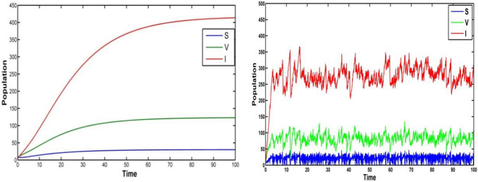
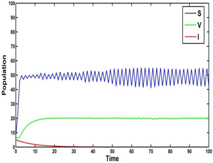
$R_0^{\ast }=\frac{\lambda }{\psi +{\alpha }_2+{\beta }_2+\frac{{\tau }_3^2}{2}}=0.00899<1$ and $\underset{t\to \infty }{lim}sup\frac{\text{ln}I\left(t\right)}{t}\le \left(\psi +{\alpha }_2+{\beta }_2+\frac{{\tau }_3^2}{2}\right)\left(R_0^{\ast }-1\right)=-0.0995<0$. It follows that Theorem 4 is verified and the epidemic will be eradicated for long run (Fig. 1). Figure 2 depicts the extinction of the system (2) for the long-term behavior.

Fig. 1.

Population trajectories in the system of (i) Deterministic system (ii) Stochastic system under the noise intensities ${\tau }_1=0.08,{\tau }_2=0.02,{\tau }_3=0.01.$

Fig. 2.

Extinction of the compartment of $I\left(t\right)$ under the noise ${\tau }_1=0.08,{\tau }_2=0.02,{\tau }_3=0.01$ and the other parameters $\left(p,q,\lambda ,k_1,\psi ,{\alpha }_1,{\alpha }_2,{\beta }_1,{\beta }_2\right)=\left(2,50,0.00009,0.65,0.02,0.9,0.03,0.2,0.05\right)$

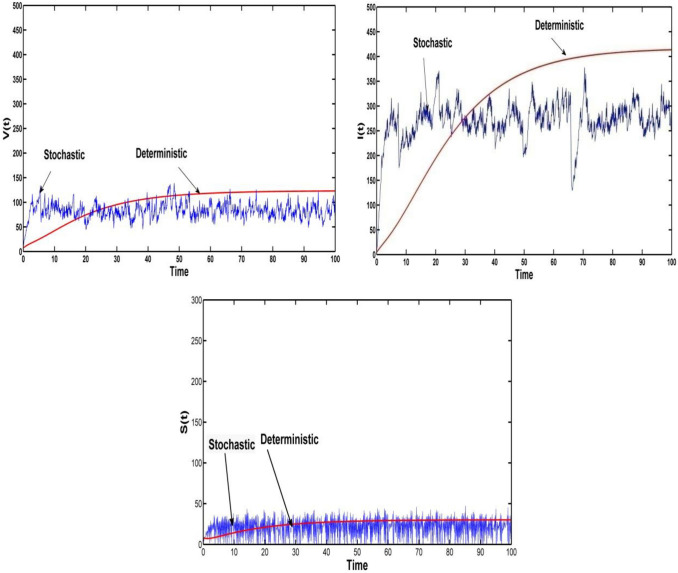
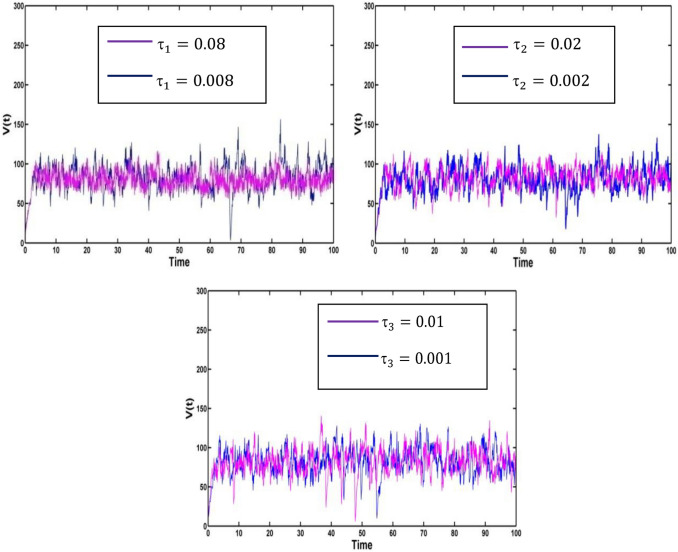
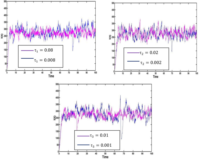
Figure 3 depicts the impact of random noises ${\tau }_i\left(i=1,2,3\right)$ on all compartment of $S\left(t\right),V\left(t\right),I\left(t\right)$ and Fig. 4 and Fig. 5 represent the effect of the noise intensities of ${\tau }_1,{\tau }_2,{\tau }_3$ on the compartment of $V\left(t\right),I\left(t\right)$. The stochastic perturbations are.

• (i)${\tau }_1=0.08,{\tau }_2=0.02,{\tau }_3=0.01$ ii)${\tau }_1=0.008,{\tau }_2=0.02,{\tau }_3=0.01$
• (iii)${\tau }_1=0.08,{\tau }_2=0.002,{\tau }_3=0.01$ iv) ${\tau }_1=0.08,{\tau }_2=0.02,{\tau }_3=0.001$, respectively.

Fig. 3.

Profile of the compartment $S\left(t\right),V\left(t\right),I\left(t\right)$ in deterministic system and stochastic system with intensities ${\tau }_1=0.08,{\tau }_2=0.02$, ${\tau }_3=0.01$ and other parameters are $\left(p,q,\lambda ,k_1,\psi ,{\alpha }_1,{\alpha }_2,{\beta }_1,{\beta }_2\right)=\left(2,50,0.9,0.65,0.02,0.9,0.03,0.2,0.05\right).$

Fig. 4.

Effect of the noise intensities ${\tau }_1,{\tau }_2,{\tau }_3$ on the compartment of $V\left(t\right)$

Fig. 5.

Effect of the noise intensities ${\tau }_1,{\tau }_2,{\tau }_3$ on the compartment of $I\left(t\right)$

For all the above cases, Fig. 3 and Fig. 4 represent the existence of a stationary distribution. The stationary distribution has an ergodicity property. But we mainly concentrate on the compartment of $V\left(t\right)$ and $I\left(t\right).$ When the perturbation intensities of vaccinated population or the infected population (${\tau }_2$ or ${\tau }_3$) increase, then the disease infection will be controlled.

Sensitivities of the parameters

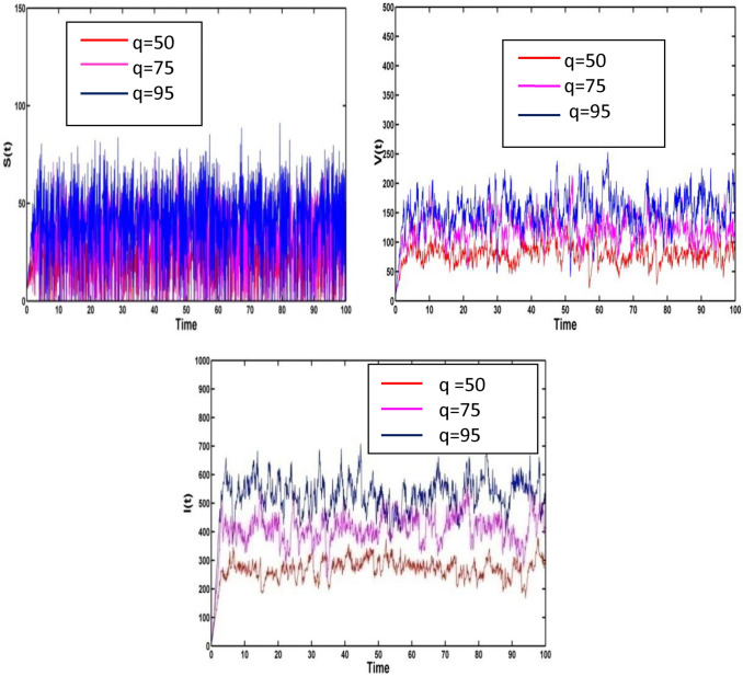
In this section, we have discussed the sensitivities of the biological parameters which influence greatly for all compartment. We consider that the epidemiological parameters are $\left(p,q,\lambda ,k_1,\psi ,{\alpha }_1,{\alpha }_2,{\beta }_1,{\beta }_2\right)=\left(2,50,0.9,0.65,0.02,0.9,0.03,0.2,0.05\right)$ and the random noises are ${\tau }_1=0.08,{\tau }_2=0.02$, and ${\tau }_3=0.01$. For the corresponding carrying capacity of the susceptible individuals $q=50,q=75,q=95$, the solutions $S\left(t\right),V\left(t\right)$ and $I\left(t\right)$ of the system (2) are presented in Fig. 6. Vaccinated population increases as carrying capacity increases. That implies disease infection can be controlled.

Fig. 6.

Effect of all the compartment $\left(S\left(t\right),V\left(t\right),I\left(t\right)\right)$ for the parameter $q$

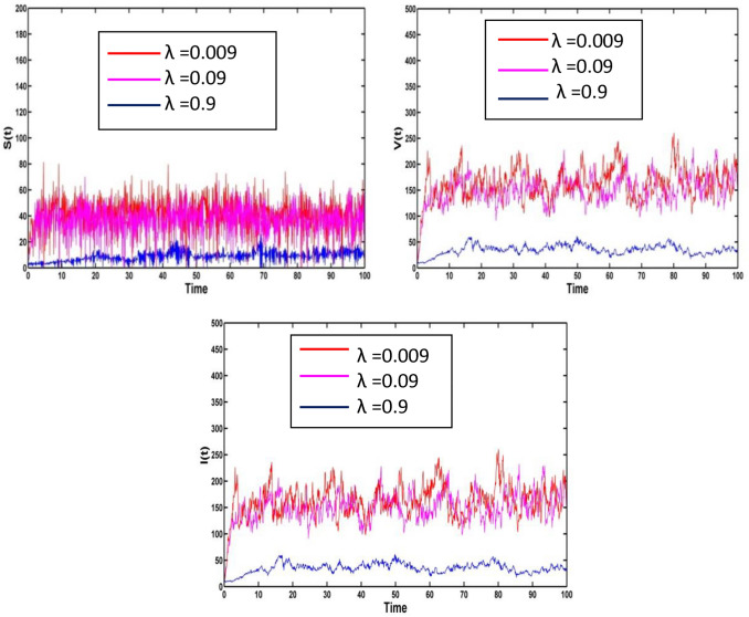
Figure 7 depicts the effect of all compartment for the different values of disease transmission rate. For the stochastic perturbation $\left({\tau }_1,{\tau }_2,{\tau }_3\right)=\left(0.08,0.02,0.01\right)$, the ecological parameters $\left(p,q,k_1,\psi ,{\alpha }_1,{\alpha }_2,{\beta }_1,{\beta }_2\right)=\left(2,50,0.65,0.02,0.9,0.03,0.2,0.05\right)$ and the disease transmission rate $\lambda =0.9,0.09,0.009$ the corresponding population intensities of susceptible, vaccinated and infected are presented in Fig. 7. The infection will decrease as the disease transmission rate increases.

Fig. 7.

Impact of all the compartment for the parameter $\lambda$

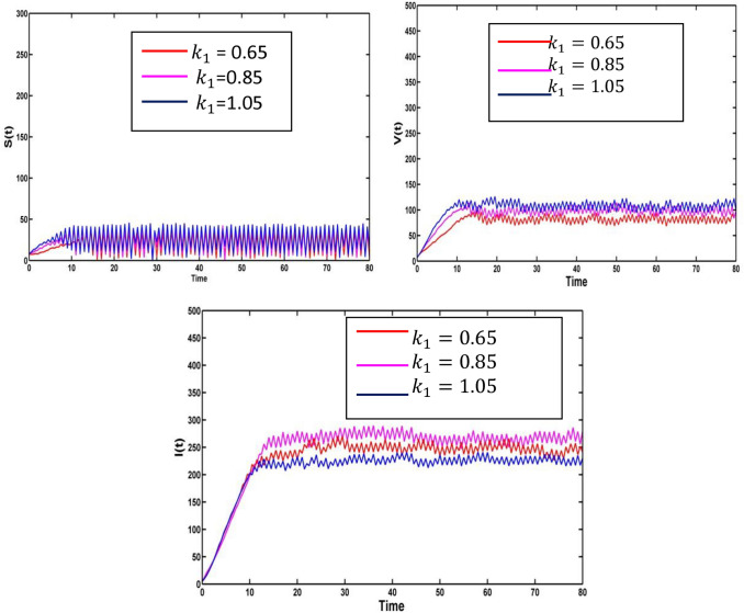
Choose the epidemiological parameter $\left(p,q,\lambda ,\psi ,{\alpha }_1,{\alpha }_2,{\beta }_1,{\beta }_2\right)=\left(2,50,0.9,0.02,0.9,0.03,0.2,0.05\right)$ and the random noises $\left({\tau }_1,{\tau }_2,{\tau }_3\right)=\left(0.08,0.02,0.01\right)$. Consider the saturation constant $k_1=0.65,0.85,1.05$, the corresponding population number of susceptible, vaccinated and infected individuals is represented in Fig. 8. The saturation rate is inversely proportional to infected individuals, i.e., the saturation increases, and then, the epidemic infection decreases.

Fig. 8.

Impact of all the compartment for the parameter $k_1$

Discussion of results

In this study, to the best of our knowledge, we establish the extinction of disease and disease persistence of the SVIS epidemic model, which adds the existence of ergodic stationary distribution and analysis of probability density function. The main study will be delivered in the following ways.

• With the linear random fluctuation (Cai and Kang 2015; Zhao and Jiang 2014; Khan and Khan 2018; Zhang 2017; Caraballo et al. 2020; Wang and Jiang 2019; Wang and Wang 2018; Liu et al. 2019a; Zhou et al. 2020, 2021; Qi and Jiang 2020; Li et al. 2010), we emphasize on SVIS epidemic model in stochastic nature with saturated incidence and vaccination strategies. With the help of Lyapunov functions, we derive the stochastic critical value $R_S^{\ast }$. Under $R_S^{\ast }>1$, a unique ergodic stationary distribution is obtained of the system (2) by the Khas’minskii theory. As the same expression of $R_S^{\ast }$ and basic reproduction number $R^{\ast }$, the dynamical properties of susceptible, vaccinated, infected individuals determine the stochastic positive equilibrium state. In the present study, ${\tau }_1,{\tau }_2,{\tau }_3$ are their corresponding random fluctuations. By using numerical results and sensitivities of parameters, we discuss some important measure to control the infectious disease.

• We cannot determine the clear view of statistical nature of disease persistence from the existence of ergodic stationary distribution. With the help Zhou et al. (Zhou et al. 2020), some algebraic equations are improved by the three-dimensional probability density function. The existence of stationary distribution with ergodic properties can obtain the corresponding persistence in the studies (Ma et al. 2015; Liu et al. 2019b). We obtain the expression of log-normal three-dimensional density function $\mathcal{T}\left(h_1,h_2,h_3\right).$ Using the algebraic equation $Y^2+B\rho +\rho B^T=0$, we solve the covariance matrix $\rho .$ It is more difficult to obtain $\rho$. Then, some standard matrices $R_1,R_2,R_3$ are taken. We can investigate the matrix $\rho$ is positive definite and the diffusion matrix $W_0$ is semi-positive definite.

For our future scope, we should add another population for recovered and analyze the disease persistence and the existence of ergodic stationary distribution. By considering the important effect of telegraph noises (Zhang et al. 2016) into the system and regime switching can be studied. It is expected that this task can be solved in later research work.

Appendix 1

Ecological description of the parameters and its units.

Parameters	Description	Unit
$\mathit{p}$	Intrinsic growth rate	day−1
$\mathit{q}$	Carrying capacity of the susceptible individuals	Human/area
$\mathit{\lambda }$	Disease transmission rate between susceptible and infected individuals	day−1
${\mathit{k}}_1$	Saturation constant	Cell/ml
$\mathit{\psi }$	Natural death rate	day−1
${\mathit{\alpha }}_1$	Vaccination rate of susceptible population	day−1
${\mathit{\alpha }}_2$	Death rate due to disease	day−1
${\mathit{\beta }}_1$	Immunity loss coefficient of vaccinated individuals	day−1
${\mathit{\beta }}_2$	Recovery rate of infected individuals	day−1

Appendix 2

The basic reproduction number $R^{\ast }$ can be computed by using the concept of next-generation matrix method (Driessche and Watmough 2002).

Let $Z={\left(I,V,S\right)}^T$, the deterministic system (1) can be written as

$$\frac{\mathit{dZ}}{\mathit{dt}}=T_1\left(z\right)-T_2\left(z\right)$$

where $T_1\left(z\right)=\left(\begin{array}{c}\frac{\lambda SI}{1+k_{1}I}\\ 0\\ 0\end{array}\right),T_2\left(z\right)=\left(\begin{array}{c}\left(\psi +{\alpha }_2+{\beta }_2\right)I\\ -{\alpha }_{1}S+\left({\beta }_1+\psi \right)V\\ \frac{\lambda SI}{1+k_{1}I}+\psi S+{\alpha }_{1}S-{\beta }_{2}I-{\beta }_{1}V-pS\left(1-\frac{S}{q}\right)\end{array}\right)$

Jacobian matrix of $T_1\left(z\right)$ & $T_2\left(z\right)$ at the disease-free equilibrium $E^{\#}=\left(S^{\#},V^{\#},I^{\#}\right)=\left[\frac{q}{p}\left\{\frac{\left(p-\psi -{\alpha }_1\right)\left({\beta }_1+\psi \right)+{\beta }_1{\alpha }_1}{{\beta }_1+\psi }\right\},\frac{{\alpha }_1}{({\beta }_1+\psi )}\frac{q}{p}\left\{\frac{\left(p-\psi -{\alpha }_1\right)\left({\beta }_1+\psi \right)+{\beta }_1{\alpha }_1}{{\beta }_1+\psi }\right\},0\right]$

$J(T_1\left(z\right))=\left(\begin{array}{cc}F& 0\\ 0& 0\end{array}\right)$ and $J(T_2\left(z\right))=\left(\begin{array}{cc}{V}_1& 0\\ J_3& J_4\end{array}\right)$.where $F=\lambda S^{\#}$, $V_1=\left(\begin{array}{cc}\psi +{\alpha }_2+{\beta }_2& 0\\ 0& {\beta }_1+\psi \end{array}\right)$, $J_3=\left(\lambda S^{\#}-{\beta }_2,-{\beta }_1\right)$,

$$J_4={\left(-{\alpha }_1,\psi +{\alpha }_1-p+\frac{2p{S}^{\#}}{q}\right)}^T$$

The basic reproduction number $\left(R^{\ast }\right)$ of the deterministic system is defined by the spectral radius of the matrix $\left(F.V_1^{-1}\right)=\frac{\lambda S^{\#}}{\left(\psi +{\alpha }_2+{\beta }_2\right)}=\frac{\lambda }{\left(\psi +{\alpha }_2+{\beta }_2\right)}\frac{q}{p}\left\{\frac{\left(p-\psi -{\alpha }_1\right)\left({\beta }_1+\psi \right)+{\beta }_1{\alpha }_1}{{\beta }_1+\psi }\right\}.$

Appendix 3

Let us assume that $\left\{\mathrm{\Omega },\mathrm{\Theta },{\left\{{\mathrm{\Theta }}_t\right\}}_{t\ge 0},\mathbb{P}\right\}$ be the complete probability space with filtration ${\left\{{\mathrm{\Theta }}_t\right\}}_{t\ge 0}$ satisfying the usual conditions (i.e., it is increasing and right continuous when ${\mathrm{\Theta }}_0$ contains all $\mathbb{P}$ null sets). For detailed study, the researcher is referred to Mao (Mao 1997). To explain the dynamical behavior of the stochastic system (2), some useful notations are defined in that space. Let us assume that ${\mathbb{R}}^n$ denotes the Euclidean space with $n$ dimension. We represent

$${\mathbb{R}}_{+}^m=\{\left(\left(y_1,\dots ..,y_m\right)\right|y_t>0,1\le t\le m\},$$

$${\mathrm{\Pi }}_{m,3}=\left(\frac{1}{m},m\right)\times \left(\frac{1}{m},m\right)\times \left(\frac{1}{m},m\right)$$

and let $B^t$ and $B^{-1}$ be the transpose matrix and inverse matrix of $B$, respectively.

Now, we choose the $m$ -dimensional stochastic differential equation.$dY\left(t\right)=g\left(Y\left(t\right),t\right)dt+h(\left(Y\left(t\right),t\right)dG\left(t\right)$ for $t\ge t_0$ and it satisfies the initial data $Y\left(0\right)=Y_0\in {\mathbb{R}}^m.$ The function $G\left(t\right)$ represents a $m$ -dimensional standard Brownian motion defined in that space. The differential operator $\mathcal{L}$ is defined by

$$\mathcal{L}=\frac{\partial }{\partial t}+\sum _{i=1}^m{g}_i\left(Y\left(t\right),t\right)\frac{\partial }{\partial Y_i}+\frac{1}{2}\sum _{i,j=1}^m{[h^T\left(Y\left(t\right),t\right)h\left(Y\left(t\right),t\right)]}_{\mathit{ij}}\frac{{\partial }^2}{\partial Y_i\partial Y_j}.$$

Here, the operator $\mathcal{L}$ is considered on a function $V\in C^{2.1}\left({\mathbb{R}}^m\times \left[t_0,\infty \right);\left[0,\infty \right)\right).$ Then, we have

$$\mathcal{L}V\left(Y,t\right)=V_t\left(Y\left(t\right),t\right)+V_Y\left(Y\left(t\right),t\right)g\left(Y\left(t\right),t\right)+\frac{1}{2}trace[h^T\left(Y\left(t\right),t\right)V_{\mathit{YY}}\left(Y\left(t\right),t\right)h\left(Y\left(t\right),t\right)],$$

where $V_t=\frac{\partial V}{\partial t},$ $V_Y=\left(\frac{\partial V}{\partial y_1},...,\frac{\partial V}{\partial y_m}\right)$ and $V_{\mathit{YY}}={\left(\frac{{\partial }^{2}V}{\partial y_i\partial y_j}\right)}_{m\times m}.$ If $Y\left(t\right)\in {\mathbb{R}}^m,$ we get

$$dV\left(Y\left(t\right),t\right)=\mathcal{L}V\left(Y\left(t\right),t\right)dt+V_Y\left(Y\left(t\right),t\right)h\left(Y\left(t\right),t\right)dG\left(t\right).$$

Declarations

Conflict of interest

The authors declare that they have no conflict of interest.

References

- Arino J, Wang L, Wolkowicz GSK. An alternative formulation for a delayed logistic equation. J Theo Biol. 2006;241:109–119. doi: 10.1016/j.jtbi.2005.11.007. [DOI] [PubMed] [Google Scholar]
- Batabyal B, Batabyal A. Mathematical computations on epidemiology: a case study of the novel coronavirus (SARS-CoV-2) Theory Biosci. 2021;140:123–138. doi: 10.1007/s12064-021-00339-5. [DOI] [PMC free article] [PubMed] [Google Scholar]
- Cai Y, Kang Y. A stochastic epidemic model incorporating media coverage. Commun Math Sci. 2015;14:893–910. doi: 10.4310/CMS.2016.v14.n4.a1. [DOI] [Google Scholar]
- Cai L, Wu J. Analysis of an HIV/AIDS treatment model with a nonlinear incidence. Chaos Soliton Fractals. 2009;41:175–182. doi: 10.1016/j.chaos.2007.11.023. [DOI] [Google Scholar]
- Caraballo T, Fatini ME, Khalifi ME. Analysis of a stochastic distributed delay epidemic model with relapseand Gamma distribution kernel. Chaos Soliton Fractals. 2020;133:109643. doi: 10.1016/j.chaos.2020.109643. [DOI] [Google Scholar]
- Carter E, Currie CC, Asuni A. The first six weeks setting up a UK urgent dental care centre during the COVID-19 pandemic. Br Dent J. 2020;228:842–848. doi: 10.1038/s41415-020-1708-2. [DOI] [PMC free article] [PubMed] [Google Scholar]
- Chong NS, Tchuenche JM, Smith RJ. A mathematical model of avian influenza with half-saturated incidence. Theory Biosci. 2014;133:23–38. doi: 10.1007/s12064-013-0183-6. [DOI] [PubMed] [Google Scholar]
- Das S, Mahato P, Mahato SK, Pal D. A mathematical study of pandemic COVID-19 virus with special emphasis on uncertain environment. J Appl Nonlinear Dyn. 2021;11:427–457. [Google Scholar]
- Gao S, Ouyang H, Nieto J. Mixed vaccination strategy in SIRS epidemic model with seasonal variability on infection. Int J Biomath. 2011;4:473–491. doi: 10.1142/S1793524511001337. [DOI] [Google Scholar]
- Higham DJ. An algorithmic introduction to numerical simulation of stochastic differential equations. SIAM Rev. 2001;43:525–546. doi: 10.1137/S0036144500378302. [DOI] [Google Scholar]
- Hove-Musekwa SD, Nyabadza F. The dynamics of an HIV/AIDS model with screened disease carriers. Comput Math Methods Med. 2009;10:287–305. doi: 10.1080/17486700802653917. [DOI] [Google Scholar]
- Iwami S, Takeuchi Y, Liu X. Avian-human influenza epidemic model. Math Biosci. 2007;207:1–25. doi: 10.1016/j.mbs.2006.08.001. [DOI] [PubMed] [Google Scholar]
- Jerubet R, Kimathi G. Analysis and modeling of tuberculosis transmission dynamics. J Adv Math Comput Sci. 2019;32:1–14. doi: 10.9734/jamcs/2019/v32i530159. [DOI] [Google Scholar]
- Jiang DQ, Zhang BX, Wang DH, Shi NZ. Existence, uniqueness, and global attractivity of positive solutions and MLE of the parameters to the logistic equation with random perturbation. Sci China Ser A-Math. 2007;50:977–986. doi: 10.1007/s11425-007-0071-y. [DOI] [Google Scholar]
- Kermack WO, McKendrick AG. A contribution to the mathematical theory of epidemics. Proc R Soc Lond A. 1927;115:700–721. doi: 10.1098/rspa.1927.0118. [DOI] [Google Scholar]
- Khan T, Khan A. The extinction and persistence of the stochastic hepatitis B epidemic model. Chaos Soliton Fractals. 2018;108:123–128. doi: 10.1016/j.chaos.2018.01.036. [DOI] [Google Scholar]
- Lee BH, Ibrahim RA. Stochastic bifurcation in non-linear structural systems near 1: 1 internal resonance. Probabilistic Eng Mech. 1994;9(1–2):23–32. doi: 10.1016/0266-8920(94)90026-4. [DOI] [Google Scholar]
- Kuniya T, Wang J. Global dynamics of an SIR epidemic model with nonlocal diffusion. Nonlinear Anal Real World Appl. 2018;43:262–282. doi: 10.1016/j.nonrwa.2018.03.001. [DOI] [Google Scholar]
- Lee H, Lao A. Transmission dynamics and control strategies assessment of avian influenza A (H5N6) in the philippines. Infect Dis Model. 2018;3:35–59. doi: 10.1016/j.idm.2018.03.004. [DOI] [PMC free article] [PubMed] [Google Scholar]
- Li MY, Smith HL, Wang L. Global dynamics of an SEIR epidemic model with vertical transmission. SIAM J Appl Math. 2001;62:58–69. doi: 10.1137/S0036139999359860. [DOI] [Google Scholar]
- Li MY, Shuai Z, Wang C. Global stability of multi-group epidemic models with distributed delays. J Math Anal Appl. 2010;361:38–47. doi: 10.1016/j.jmaa.2009.09.017. [DOI] [Google Scholar]
- Li J, Teng Z, Wang G, Zhang L, Hu C. Stability and bifurcation analysis of an SIR epidemic model with logistic growth and saturation treatment. Chaos Solit Fractals. 2017;99:63–71. doi: 10.1016/j.chaos.2017.03.047. [DOI] [Google Scholar]
- Lipster RA. Strong law of large numbers for local martingales. Stochastics. 1980;3:217–228. doi: 10.1080/17442508008833146. [DOI] [Google Scholar]
- Liu X, Takeuchi Y, Iwami S. SVIR epidemic models with vaccination strategies. J Theor Biol. 2008;253:1–11. doi: 10.1016/j.jtbi.2007.10.014. [DOI] [PubMed] [Google Scholar]
- Liu Q, Jiang D, Hayat T, Ahmad B. Analysis of a delayed vaccinated SIR epidemic model with temporary immunity and Lévy jumps. Nonlinear Anal Real. 2018;27:29–43. doi: 10.1016/j.na.2017.10.011. [DOI] [Google Scholar]
- Liu Q, Jiang D, Hayat T, Alsaedi A. Dynamical behavior of a stochastic epidemic model for cholera. J Frankl I. 2019;356:7486–7514. doi: 10.1016/j.jfranklin.2018.11.056. [DOI] [Google Scholar]
- Liu Q, Jiang D, Hayat T, Alsaedi A. Long-time behaviour of a stochastic chemostat model with distributed delay. Stochastics. 2019;91:1141–1163. doi: 10.1080/17442508.2019.1576689. [DOI] [Google Scholar]
- Ma Z, Zhou Y, Li C. Qualitative and stability methods for ordinary differential equations. Beijing: Science Press; 2015. [Google Scholar]
- Mahato P, Das S, Mahato SK. An epidemic model through information induced vaccination and treatment under fuzzy impreciseness. Model Earth Syst Environ. 2022;8:2863–2887. doi: 10.1007/s40808-021-01257-7. [DOI] [PMC free article] [PubMed] [Google Scholar]
- Mao X. Stochastic differential equations and applications. Chichester: Horwood Publishing; 1997. [Google Scholar]
- Naik PA, Zu J, Ghoreishi M. Stability analysis and approximate solution of sir epidemic model with crowley-martin type functional response and holling type-II treatment rate by using homotopy analysis method. J Appl Anal Comput. 2020;10:1482–1515. [Google Scholar]
- Naik PA, Zu J, Owolabi KM. Global dynamics of a fractional order model for the transmission of HIV epidemic with optimal control. Chaos Solitons Fractals. 2020;138:1–30. doi: 10.1016/j.chaos.2020.109826. [DOI] [PMC free article] [PubMed] [Google Scholar]
- Qi K, Jiang D. The impact of virus carrier screening and actively seeking treatment on dynamical behavior of a stochastic HIV/AIDS infection model. Appl Math Model. 2020;85:378–404. doi: 10.1016/j.apm.2020.03.027. [DOI] [Google Scholar]
- Roozen H. An asymptotic solution to a two-dimensional exit problem arising in population dynamics. SIAM J Appl Math. 1989;49:1793. doi: 10.1137/0149110. [DOI] [Google Scholar]
- Van den Driessche P, Watmough J. Reproduction numbers and sub-threshold endemic equilibria for compartmental models of disease transmission. Math Biosci. 2002;180:29–48. doi: 10.1016/S0025-5564(02)00108-6. [DOI] [PubMed] [Google Scholar]
- Vincenzo C, Gabriella S. A generalization of the Kermack–McKendrick deterministic epidemic model. Math Biosci. 1978;42:43–61. doi: 10.1016/0025-5564(78)90006-8. [DOI] [Google Scholar]
- Wang Y, Jiang D. Stationary distribution of an HIV model with general nonlinear incidence rate and stochastic perturbations. J Frankl I. 2019;356:6610–6637. doi: 10.1016/j.jfranklin.2019.06.035. [DOI] [Google Scholar]
- Wang L, Wang K. Nontrivial periodic solution for a stochastic brucellosis model with application to Xinjiang, China. Physica A. 2018;510:522–537. doi: 10.1016/j.physa.2018.06.061. [DOI] [Google Scholar]
- Xing Y, Li HX. Almost periodic solutions for a SVIR epidemic model with relapse. MBE. 2021;18:7191–7217. doi: 10.3934/mbe.2021356. [DOI] [PubMed] [Google Scholar]
- Xu R, Wang ZL, Zhang FQ. Global stability and Hopf bifurcations of an SEIR epidemiological model with logistic growth and time delay. Appl Math Comput. 2015;269:332–342. [Google Scholar]
- Xu R, Zhang S, Zhang F. Global dynamics of a delayed SEIS infectious disease model with logistic growth and saturation incidence. Math Methods Appl Sci. 2016;39:3294–3308. doi: 10.1002/mma.3774. [DOI] [Google Scholar]
- Zhang X. Global dynamics of a stochastic avian–human influenza epidemic model with logistic growth for avian population. Nonlinear Dyn. 2017;90:2331–2343. doi: 10.1007/s11071-017-3806-5. [DOI] [Google Scholar]
- Zhang X, Jiang D, Alsaedi A. Stationary distribution of stochastic SIS epidemic model with vaccination under regime switching. Appl Math Lett. 2016;59:87–93. doi: 10.1016/j.aml.2016.03.010. [DOI] [Google Scholar]
- Zhao Y, Jiang D. The threshold of a stochastic SIS epidemic model with vaccination. Appl Math Comput. 2014;243:718–727. [Google Scholar]
- Zhou B, Zhang X, Jiang D. Dynamics and density function analysis of a stochastic SVI epidemic model with half saturated incidence rate. Chaos Soliton Fractals. 2020;137:109865. doi: 10.1016/j.chaos.2020.109865. [DOI] [Google Scholar]
- Zhou B, Jiang D, Dai Y, Hayat T, Alsaedi A. Stationary distribution and probability density function of a stochastic SVIS epidemic model with standard incidence and vaccination strategies. Chaos Solitons Fractals. 2021;143:110601. doi: 10.1016/j.chaos.2020.110601. [DOI] [PMC free article] [PubMed] [Google Scholar]
- Zhu L, Wang X, Zhang H, Shen S, Li Y, Zhou Y. Dynamics analysis and optimal control strategy for a SIRS epidemic model with two discrete time delays. Phys Scr. 2020;95:035213. doi: 10.1088/1402-4896/ab495b. [DOI] [Google Scholar]