

Abstract
With the increasing awareness of the health impacts of particulate matter, there is a growing need to comprehend the spatial and temporal variations of the global abundance of ground level airborne particulate matter with a diameter of 2.5 microns or less (PM2.5). Here we use a suite of remote sensing and meteorological data products together with ground-based observations of particulate matter from 8,329 measurement sites in 55 countries taken 1997–2014 to train a machine-learning algorithm to estimate the daily distributions of PM2.5 from 1997 to the present. In this first paper of a series, we present the methodology and global average results from this period and demonstrate that the new PM2.5 data product can reliably represent global observations of PM2.5 for epidemiological studies.
Keywords: PM2.5, machine-learning, remote sensing
Introduction
Numerous studies show that among air pollutants, particulate matter (PM), especially with a diameter of 2.5 microns or less (PM2.5), has the strongest link with human health effects (Brook et al., 2010a,b, 2013a,b; Pope et al., 2011; Lary et al., 2014). Increased morbidity and mortality has been associated with exposure to PM2.5 suggesting that improved life expectancy is possible by reducing the exposure level (Pope et al., 2009). Not only in the United States of America (USA), but also in European studies, a significant number of premature deaths, including those due to cardiopulmonary and lung cancer, are attributed to long-term exposure to PM2.5 (Boldo et al., 2006, 2011; Ballester et al., 2008). The many health impacts of such particulate matter (Table 1) depend in part on its abundance at ground level in the atmospheric boundary layer where it can be inhaled.
Table 1.
Particulate matter and health outcomes for PM10, PM2.5 and ultrafine particles (UFPs).
| Health outcomes | Short-term studies | Long-term studies | ||||
|---|---|---|---|---|---|---|
| PM10 | PM2.5 | UFP | PM10 | PM2.5 | UFP | |
| Mortality | ||||||
| All causes | xxx | xxx | x | xx | xx | x |
| Cardiovascular | xxx | xxx | x | xx | xx | x |
| Pulmonary | xxx | xxx | x | xx | xx | x |
| Pulmonary effect | ||||||
| Lung function, e.g. PEF | xxx | xxx | xx | xxx | xxx | |
| Lung function growth | xxx | xxx | ||||
| Asthma and COPD exacerbation | ||||||
| Acute respiratory symptoms | xx | x | xxx | xxx | ||
| Medication use | x | |||||
| Hospital admission | xx | xxx | x | |||
| Lung cancer | ||||||
| Cohort | xx | xx | x | |||
| Hospital admission | xx | xx | x | |||
| Cardiovascular effects | ||||||
| Hospital admission | xxx | xxx | x | x | ||
| ECG-related endpoints | ||||||
| Autonomic nervous system | xxx | xxx | xx | |||
| Myocardial substrate and vulnerability | xx | x | ||||
| Vascular function | ||||||
| Blood pressure | xx | xxx | x | |||
| Endothelial function | x | xx | x | |||
| Blood markers | ||||||
| Pro inflammatory mediators | xx | xx | xx | |||
| Coagulation blood markers | xx | xx | xx | |||
| Diabetes | x | xx | x | |||
| Endothelial function | x | x | xx | |||
| Reproduction | ||||||
| Premature birth | x | x | ||||
| Birth weight | xx | x | ||||
| IUR/SGA | x | x | ||||
| Fetal growth | ||||||
| Birth defects | x | |||||
| Infant mortality | xx | x | ||||
| Sperm quality | x | x | ||||
| Neurotoxic effects | ||||||
| Central nervouse system | x | xx | ||||
x = few studies (6 or less); xx = many studies (7–10); xxx = large number of studies (>10).
For more than half a century, researchers have been studying the impact of PM on health. Initially the attempt was to learn about the possible adverse effects; then the focus shifted to investigate the exposure-response relationships. With further advancement in technology and more awareness of health-concerns, studies on composition-specific effects have emerged (Ayala et al., 2012). With implementation of computational fluid dynamics (CFD) models and digital imaging of organs, researchers have started to study the pathophysiology associated with PM to better understand the translocation of particulates in the human body after their deposition and how they impact health.
Most short-term exposure impact studies on PM2.5, whether for morbidity or mortality, focus on cardiovascular/cardiopulmonary (Brook et al., 2010b) or respiratory (Dockery et al., 1993) conditions. Our dataset, with daily temporal scale, is suitable for such studies. We are already studying daily asthma-related hospital admissions associated with PM2.5 using our estimated data. On the other hand, diseases, such as lung cancer, require study of long-term exposure. Data generated from this study are expected to contribute to Health Impact Assessment (HIA) in different parts of the world concerning long-term exposure to PM2.5. Currently, long-term values are not available in many localities and in many instances, PM2.5 values are estimated from PM10 for long-term HIA (Boldo et al., 2011). Studies also suggest that even low-level PM2.5 exposure can contribute to serious health impacts (Pope et al., 2006; Franklin et al., 2007; Crouse et al., 2012; Cesaroni et al., 2014). We have already created daily global estimates of PM2.5 with an associated uncertainty for more than 13 years providing an appropriate dataset for extended cohort studies for the areas with both high and mid-level concentrations of ambient PM2.5. In addition, long-range transportation of particles as, such dust can provide potential vectors for bacteria (Ginoux and Torres, 2003; Prospero, 2003). With global coverage of this study, tracking PM2.5 transport is now easier for public health surveillance.
In recent years, researchers are finding it worthy to investigate potential links between PM2.5 exposure and adverse birth outcomes (Slama et al., 2008; Dadvand et al., 2013), epigenetic alteration (Baccarelli et al., 2008; Salam et al., 2012; Byun et al., 2013; Hou et al., 2013) infant mortality (Woodruff et al., 1997; Lipfert et al., 2000; Dales et al., 2004; Glinianaia et al., 2004) atherosclerosis (Araujo et al., 2008; Araujo, 2011; Kaufman, 2011), stroke (Brook, 2008; Brook and Rajagopalan, 2009, 2012; Maheswaran et al., 2010, 2012), rheumatic autoimmune disease (Zeft et al., 2009; Farhat et al., 2011), central nervous system disorders (Sunderman, 2001; Kreyling et al., 2006; Block and Calderon-Garciduenas, 2009; Pearson et al., 2010; Wang et al., 2012) and diabetes (Andersen, 2012; Andersen et al., 2012). Since many of these health conditions are interlinked, comprehensive studies are required to better understand the impact of PM2.5. With increasing availability of electronic health records, reliable PM2.5 data with seamless temporal and geographic coverage can contribute to revealing many unknowns of PM2.5 impacts on health.
It could be noted that the type and degree of adverse effect greatly depends on the composition of the particulate matters. Composition mostly varies due to source materials. Our current study does not provide information on the composition of PM2.5. However, this study can be extended to examine the potential of source apportionment considering land use / land cover conditions and transportation mechanisms. Recent studies show specific adverse impacts of exposure to ultrafine particles (UFPs). Future studies are recommended to derive further size fractions beyond just PM2.5, particularly UFPs in the sub-micron size range. Various networks of ground-based sensors routinely measure the abundance of PM2.5. However, the spatial coverage has many large gaps and in some countries no observations are made at all. Globally more observations of PM10 are available than for PM2.5. This paper focuses on PM2.5, which has been related to a wider variety of health conditions than PM10 or UFPs (Table 1).
Several studies have sought to overcome this limitation of spatial coverage by using remote sensing and satellite-derived Aerosol Optical Depth (AOD) coupled with regression and/or numerical models to estimate the ground-level abundance of PM2.5 (e.g. Engel-Cox et al., 2004a; Zhang et al., 2009, 2011; Hoff and Christopher, 2009; Weber et al., 2010). Studies have shown that the relationship between PM2.5 and AOD is not always suitable for simple regression models. Rather it is determined by a multi-variate function of a large number of parameters, including: humidity, temperature, boundary layer height, surface pressure, population density, topography, wind speed, surface type, surface reflectivity, season, land use, normalised variance of rainfall events, size spectrum and phase of cloud particles, cloud cover, cloud optical depth, cloud top pressure and the proximity to particulate sources releasing PM2.5 (Liu et al., 2005; Lyamani et al., 2006; Choi et al., 2008; Paciorek et al., 2012; Zhang et al., 2009). The picture is further complicated by the biases present in satellite AOD products (e.g. Lary et al., 2009; Hyer et al., 2011; Shi et al., 2012; Reid et al., 2013), the difference in spatial scales of the in-situ point PM2.5 observations and remote sensing data (several km per pixel) and, finally, the sharp PM2.5 gradients that can exist in and around cities.
Zhang et al. (2009) presented a comprehensive study for the ten Environmental Protection Agency (EPA) regions across USA using multi-linear regression between the PM2.5 abundance observed by the EPA monitoring sites and the Moderate Resolution Imaging Spectroradiometer (MODIS), AOD and a set of meteorological parameters. In their multi-linear regression study (Zhang et al., 2009) found the best correlations of PM2.5 with AOD in the eastern states during summer and autumn, with EPA region number 4 having a correlation coefficient of more than 0.6. They observed the poorest correlation for the south-western USA, with EPA region number 9 having a correlation coefficient of approximately 0.2. Weber et al. (2010) extended the work by Zhang et al. (2009) for five EPA monitoring sites in the Baltimore/Washington DC Metro area by considering AOD from MODIS, the Multi-Angle Imaging Spectroradiometer (MISR) and the Geostationary Operational Environmental Satellite (GOES). These PM2.5 estimates are made available through the Infusing satellite Data into Environmental Applications (IDEA) website (http://www.star.nesdis.noaa.gov/smcd/spb/aq).
In a notable study, van Donkelaar et al. (2006) took the alternative approach of using remote sensing and a global transport model to present a global estimate of the long-term average PM2.5 concentrations between the years 2001 and 2006 using satellite observations of AOD from MODIS to estimate η = PM2.5/AOD. The three-dimensional (3D) chemical transport model used was GEOS-Chem (http://acmg.seas.harvard.edu/geos/), and the authors found a significant spatial agreement with their estimates; the correlation coefficient for North American PM2.5 measurements was 0.77 and elsewhere 0.83. PM2.5 estimates using this approach have since been used in a variety of health studies (van Donkelaar et al., 2010a; Anderson et al., 2012; Brauer et al., 2012; Crouse et al., 2012; Hystad et al., 2012). Meanwhile, Liu et al. estimated the ground level abundance of PM2.5 by using scaling factors from the GEOS-Chem, GOCART models and AOD from the MISR (Liu et al., 2004, 2005, 2007a,b,c, 2009a,b,c).
This study makes five incremental contributions:
we believe we have used the most comprehensive training dataset to date for a study that empirically relates hourly in situ PM2.5 observations to remote sensing, meteorological and other contextual, environmental data. This is important as the local context of the various PM2.5 observations varies widely and in order to have a robust estimation of the global PM2.5 distribution, we need representative observations in a wide range of conditions. Hourly PM2.5 observations were acquired from 1997-present from across the world. In this study we used hourly PM2.5 data from 8,329 measurement sites in 55 countries;
we believe we have used the widest range of contextual variables to date (over 30 identified from the literature and presented in the last section) in our analysis of the measured multivariate, non-linear, non-parametric relationship between ground based observations of PM2.5 and remote sensing observations, meteorological observations and associated contextual information;
we have used the most-suitable multivariate, non-linear, non-parametric machine-learning approach currently available (briefly described in the next section) and not previously used for investigating the empirical relationship between hourly in-situ PM2.5 observations and remote sensing, meteorological and other contextual environmental data;
we not only estimate the PM2.5 abundance, but also provide an uncertainty estimate; and
we cover the longest time period estimating the PM2.5 abundance on a daily basis (from September 1, 1997 to the present).
Materials and methods
Many studies have shown that the relationship between PM2.5 and AOD is a multi-variate function of a large number of parameters (Liu et al., 2005; Lyamani et al., 2006; Choi et al., 2008; Natunen et al., 2010; Liu and Harrison, 2011). Further, many of these relationships are non-linear, some are of unknown functional form and many have non-Gaussian distributions. Therefore, any successful description of the relationship between PM2.5 and AOD needs to be multi-variate, non-parametric (we do not know the functional form from theory) and able to deal with non-linear behaviour and non-Gaussian distributed variables. This would suggest that a machine-learning algorithm should be used.
Machine-learning can provide a valuable regression tool for empirically estimating variables of interest, when we do not have a complete theoretical description of a process but do have a useful set of observations. Machine-learning encompasses a broad range of algorithms (e.g. Neural Networks, Support Vector Machines, Gaussian Processes, Decision Trees, Random Forests, etc.) that can provide multi-variate, non-linear, non-parametric regression or classification based on a training dataset. We have used all of these approaches for estimating PM2.5 and have also developed our own proprietary ensemble approach with full error estimation (a description of which is beyond the scope of this text). The key points to highlight as relevant to this study are:
the approach includes a full independent validation. A fraction of the training data is randomly selected and held back for independent validation. These validation points are shown in red in Fig. 3;
at every location we considered, the approach provides both an estimate of the PM2.5 abundance as well as an error estimate;
an ensemble of independent predictors are used at every location, and our estimate of the PM2.5 abundance is the mean of the ensemble of estimates. A full error characterisation showed that beyond an ensemble size of 6, there was no significant error reduction. However, we used an ensemble size of 12 to be completely sure we had an ensemble that was large enough;
the approach provides a ranking of the relative importance of each of the variables used in the regression;
the approach can handle records with missing values. However, in this study we chose to ignore records with missing values.
Fig. 3.
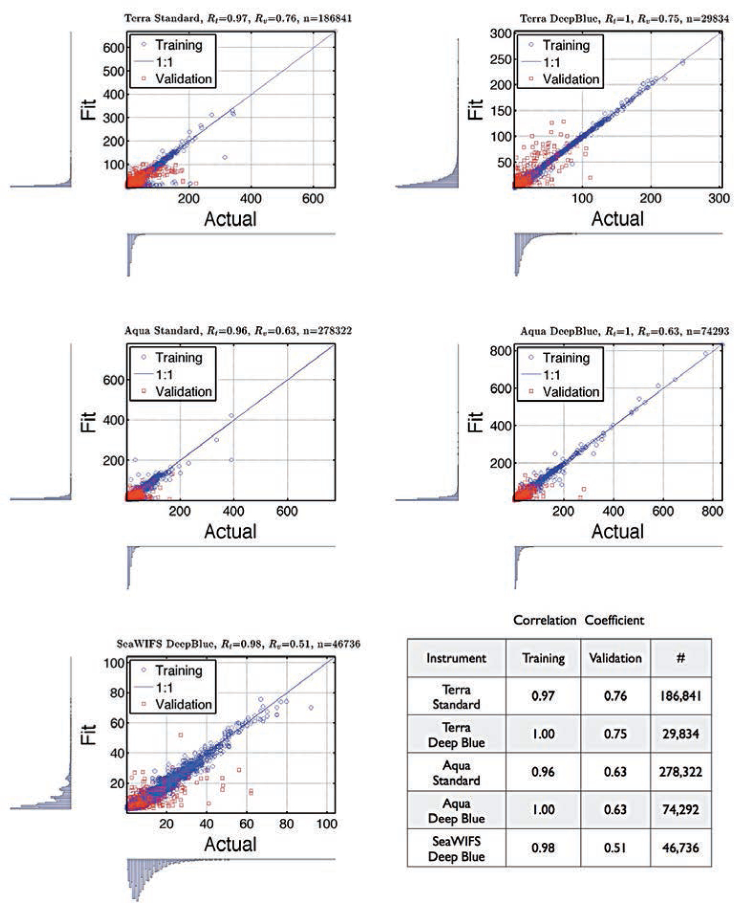
Scatter diagrams showing the hourly average PM2.5 abundance. PM2.5 load in μg/m3 on the x-axis and the machine-learning estimate (or fit) on the y-axis. The associated probability density function is also shown along each axis. The title of each plot shows the MODIS product used, the correlation coefficient for the training dataset (Rt), the correlation coefficient for the independent validation dataset (the 5% random selection of data left out of the training data set for independent validation - Rv and the sample size (n)). The blue circles represent the data used in the training and the red squares the independent validation dataset. The table insert gives the correlation coefficients in descending order of the correlation coefficient for the independent validation dataset.
Datasets used in machine-learning regression
PM2.5 data –
We used as many in-situ hourly PM2.5 observations as possible from 8,329 sites in 55 countries from August 1, 1997 to the present (shown as red squares in Fig. 1). Fig. 2 shows the spatial and temporal coverage of this training data. Most of the observation sites were in the northern hemisphere. The high-latitude satellite data coverage is greatest in summer, so the number of in-situ PM2.5 observations with satellite overpasses is greatest in summer as can be seen by the annual summer peaks in the Figure. Having training data from as many different physical environments as possible is critical, so a wide range of diverse conditions should be incorporated in the training data. The quality of the global machine-learning estimates of PM2.5 improved dramatically with the inclusion of data from the southern hemisphere (Chile, Brazil, South Africa, Australia and New Zealand) and Asia (China, India, Japan, Taiwan and Hong Kong). A random sample comprising 5% of each training dataset was held back for independent evaluation of the PM2.5 estimate produced using machine-learning.
Fig. 1.
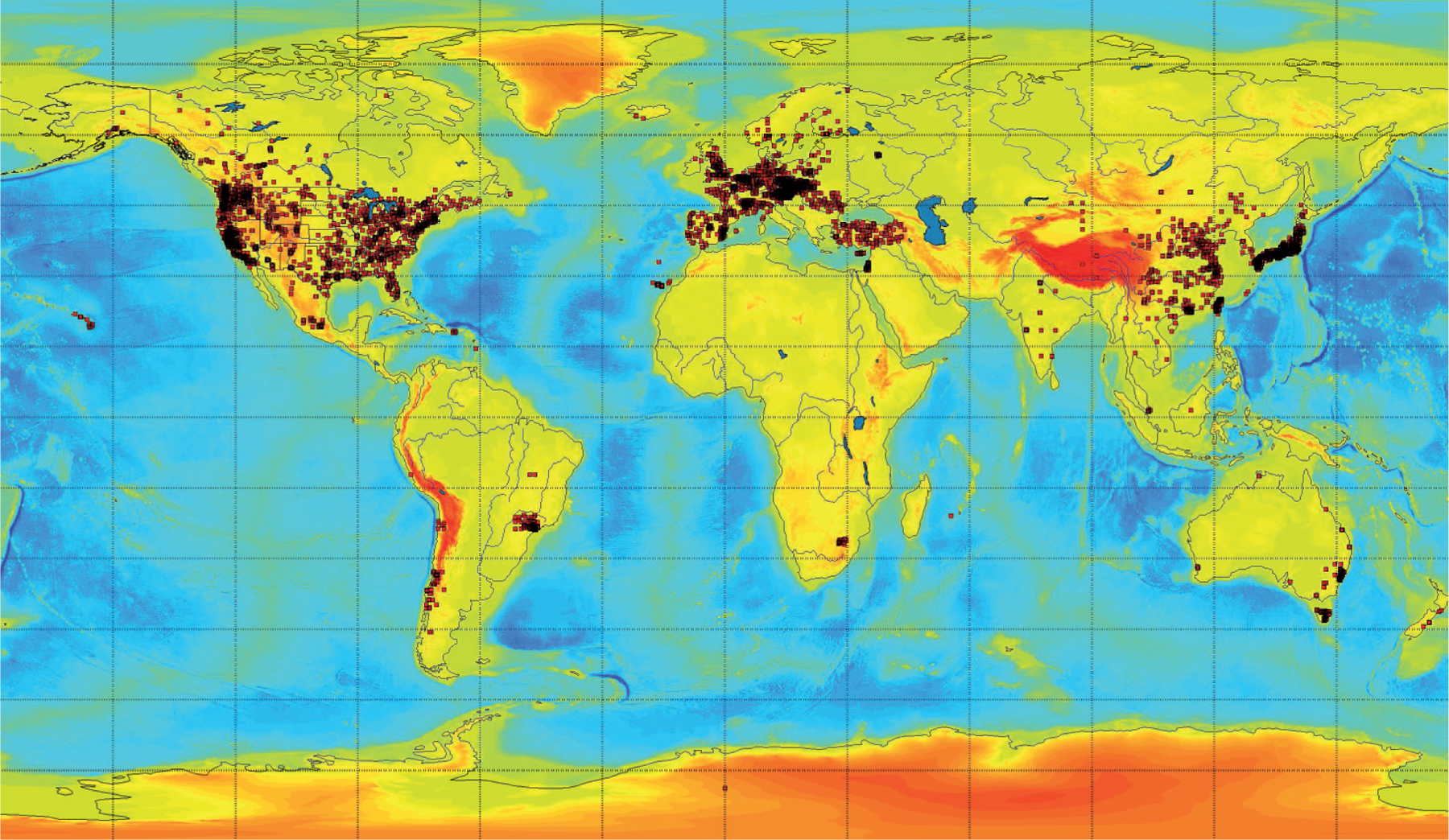
Map showing the 8,329 PM2.5 measurement site locations from 55 countries studied 1997–2014. Black squares show sites, where measurements were made against the background colour scale of global topography and bathymetry. North America, Europe and Asia have the greatest density of sites but there are also southern hemisphere sites in South America, South Africa, Australia and New Zealand.
Fig. 2.
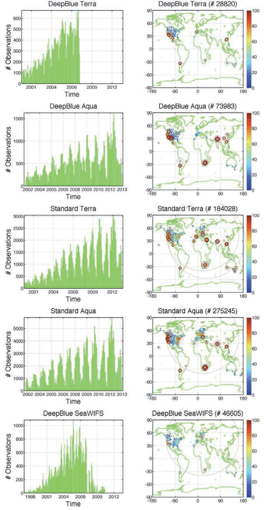
Temporal (left) and spatial distribution (right) of the training data. The temporal range is different for each instrument and algorithm combination. The size of the symbols in the panels to the right is proportional to the PM2.5 abundance.
Satellite AOD data –
This study used satellite data from three satellite instruments: the Sea-viewing Wide Field-of-view Sensor (SeaWIFS) launched on August 1, 1997 (Melin et al., 2013). Two MODIS instruments (one onboard the Terra satellite (EOS AM) launched in 1999, the other on Aqua (EOS PM) launched in 2002) (Remer et al., 2008) were chosen, both for their coverage and their near-real time data delivery. The latest distribution of MODIS data collection 5.1 was used. In this study we used the level 2 collection 5.1 data and a spatial grid with a resolution of 10 × 10 km (approximately 0.1° × 0.1°). MODIS collection 5 introduced the Deep Blue algorithm for retrieval of AOD over bright arid surfaces, an approach based on the idea that desert regions are darker at shorter wavelengths so the aerosol signal is clearer when using the shorter deep blue wavelengths (Hsu et al., 2004, 2006; Sayer et al., 2013).
The MODIS aerosol data files are called MOD04 for Aqua and MYD04 for Terra. In addition to the MODIS aerosol optical depth over land and ocean, the product data files include the viewing and solar illumination geometries, surface reflectance, scattering angle, angstrom exponent and various quality and cloud flags. These additional parameters turned out to be invaluable in providing an accurate multivariate, non-parametric regression to estimate the surface abundance of PM2.5.
In MODIS collection 5.1, Deep Blue Terra data are not available after 2007. When collection 6 is released this should be remedied, there will be greater Deep Blue data coverage and higher spatial resolution. Collection 6 will include various refinements to Deep Blue, including extended coverage to vegetated and bright land surfaces, improved cloud screening and surface reflectance and aerosol microphysical models. Many of these improvements were developed during the recent application of Deep Blue to SeaWiFS data.
Meteorological data –
The meteorological data used in this study come from the NASA Modern Era Retrospective analysis for Research and Applications (MERRA) (http://gmao.gsfc.nasa.gov/merra/) (Rienecker et al., 2011). The historic data are available from the Modeling and Assimilation Data and Information Services Center (MDISC) at http://disc.sci.gsfc.nasa.gov/mdisc/. The real-time and forecast data are available as part of the experimental forecast suite at http://gmao.gsfc.nasa.gov/forecasts/.
PM2.5 product evaluation
Let us now evaluate the quality of the machine-learning regression using several different approaches.
Scatter diagrams –
Scatter diagrams using data for the entire period of 1997 to present provide a visual means for evaluating the quality of the estimated PM2.5 abundance. A perfect fit would yield a scatter diagram with a slope of one and an intercept of zero. Fig. 3 shows scatter diagrams of the observed in-situ hourly average PM2.5 abundance in μg/m3 on the x-axis and the machine-learning estimate on the y-axis. The blue circles depict the training dataset and the red squares the randomly chosen independent validation dataset; the associated probability density function is shown along each axis. The title of each panel shows the satellite data product used, the correlation coefficient for the independent training dataset Rt, the correlation coefficient for the independent validation dataset Rv and the sample size n. The table tabulates the correlation coefficients in descending order of Rv. It should be noted that the correlation coefficient for each of the five training datasets is 0.96 or greater and that the estimates (blue circles) are tightly clustered about the 1:1 line. The correlation coefficient for each of the independent validation datasets (red squares) is 0.52 or greater and, as would be expected, there is a little more scatter. We see that the quality varies slightly by satellite with the best fits obtained from Terra data, followed by Aqua and then SeaWIFS.
Quintile-Quintile plots -
these permit comparison between the shapes of the observed and the estimated probability density functions. Two probability density functions of the same shape yield a straight line. For a good agreement we expect at least the 25th to 75th quintiles (the “overplotted” red squares) to form a straight line as it does for our machine-learning fits of the PM2.5 abundance.
The probability density functions (PDF) are shown along each axis of the scatter diagrams in Fig. 3. We can see that the PDFs of the in-situ observations and our machine-learning estimates have very similar shapes. The relative shapes of the independent validation PDFs are further tested graphically using quintile-quintile plots (Fig. 4). The observed PM2.5 abundance quintiles are plotted on the x-axis and the machine-learning estimated PM2.5 abundance quintiles for the independent validation dataset on the y-axis. Typically the 25th to 75th quintiles of globally observed PM2.5 abundance falls in the range of 5–20 μg/m3. The extremely polluted areas in Asia and around some large cities are outliers (falling above the 75th quintile) in the global PM2.5 abundance PDF.
Fig. 4.
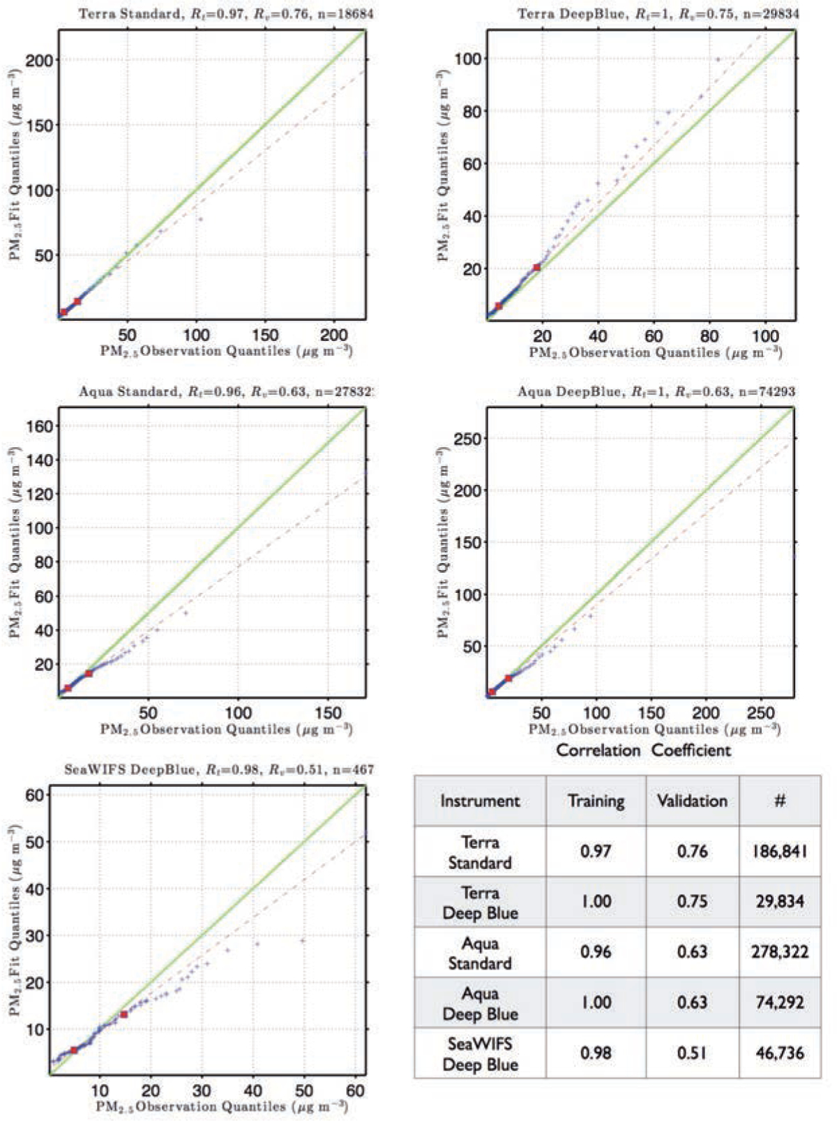
Quintile-quintile diagrams for the independent validation data showing the observed quintiles of in-situ hourly average PM2.5 abundance. PM2.5 abundance in μg/m3 on the x-axis and the machine-learning estimated quintiles on the y-axis. The blue circles represent the data used in the training and the red squares the independent validation dataset. The table insert gives the correlation coefficients in descending order for the independent validation dataset. Every percentile between 1 and 100 plotted.
If the quintile-quintile plot is a straight line y = ax + b, but the slope is not 1. This means that the machine-learning fit and the observed data distributions differ slightly in their location and scale (Chambers et al., 1983; Fowlkes, 1987). The slope and intercept provide estimates of the scale and location. In our case the left end of the pattern is generally slightly above the 1:1 line and the right end of the pattern is slightly below the line indicating that the PDF for the machine-learning fit has slightly shorter tails at each end of the distribution when compared to the PDF of the observations. In most cases the machine-learning approach slightly underestimates the largest PM2.5 abundances, but agrees with in-situ observations to within the estimated uncertainty.
Taylor diagrams –
This type of graph, intoduced by Taylor (2001) provides another visual way to compare the machine-learning fit to the hourly average PM2.5 abundance in μg/m3 to the observations (Fig. 5). The Taylor diagram quantifies the similarity between the fit and observations based on the correlation coefficient, the centred root-mean-square (RMS) difference between the fit and observations and the amplitude of their variations using the standard deviation. In each case the observations are denoted by point A on the x-axis. The green contours shown around A indicate the centred RMS differences between the fit and observations. The radial distance of a point from the origin is proportional to the amplitude of variation quantified by the standard deviation. Points lying on a radial arc the same distance from the origin as point A have the same standard deviation as the observations indicating that the simulated variations have the correct amplitude. We can see from Fig. 5 that all the machine-learning fits are of reasonable quality, but those using the Deep Blue data simulate the amplitude of variation seen in the observations better than the standard algorithm.
Fig. 5.
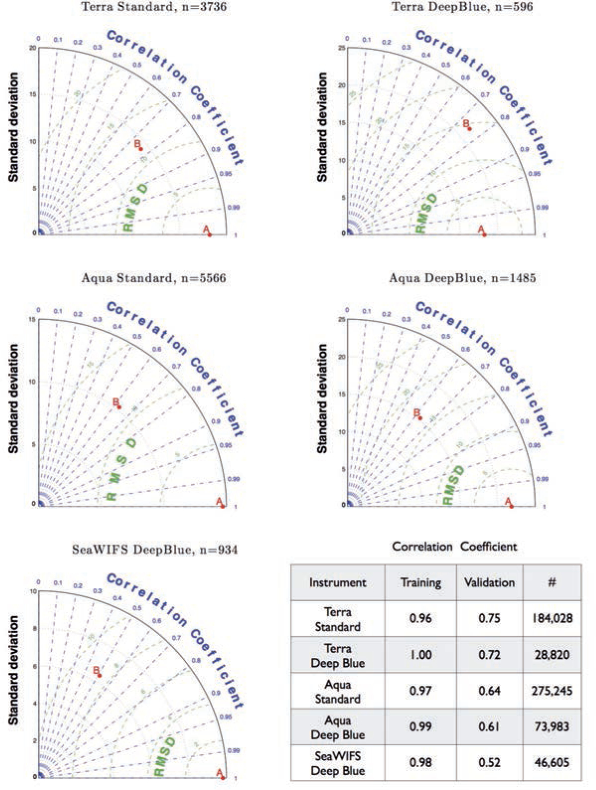
Taylor diagrams quantify the similarity between the fit and observations and the amplitude of their variations, i.e. the similarity between fit and observations based on the correlation coefficient and the centred RMS difference on the one hand, and the amplitude of their variations using the standard deviation on the other. In each case, the observations are denoted by point A on the x-axis. The green contours around A show the centred RMS differences between fit and observations. The radial distance of a point from the origin is proportional to the amplitude of variation quantified by the standard deviation. Points lying on a radial arc, at the same distance from the origin as point A, have the same standard deviation indicating that the simulated variations have the correct amplitude.
Ensemble errors –
Fig. 6 shows the ensemble training errors in μg/m3 for our PM2.5 abundance estimates. The blue lines show the RMS error evaluated for the training dataset and the red lines show the RMS error for the independent validation dataset. The ensemble training errors depend on how many members are in the machine-learning ensemble. There is a decrease in the error between one and six ensemble members that then plateaus with little benefit in having more than fifteen learners. In this study we have used an ensemble size of twelve.
Fig. 6.
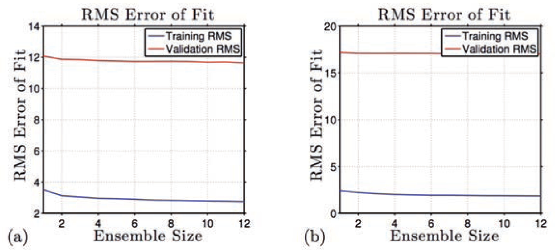
Ensemble training errors in μg/m3 for the Aqua Standard machine-learning PM2.5 estimates (a), and the Aqua Deep Blue machine-learning PM2.5 estimates (b). The blue lines show the RMS error evaluated for the training dataset, and the red lines the RMS error for the independent validation dataset.
Multi-annual estimate of PM2.5 abundance
A useful validation of the new PM2.5 data product is to survey the key features of the global PM2.5 distribution and see if they capture, what we expect to find, and what has been reported in the literature. The upper panel of Fig. 7 shows the global average of the surface PM2.5 abundance estimated using machine-learning of the 5,874 daily estimates from August 1 1997 to August 31 2013 in μg/m3. Overlaid as colour-filled circles are the observations for those locations, for which we have both a machine-learning estimate of the surface PM2.5 abundance and an observation for at least one third of the 5,874 days between August 1, 1997 to August 31, 2013. The agreement between the machine-learning estimate and the in-situ observations is well within the estimated uncertainty shown in the lower panel.
Fig. 7.
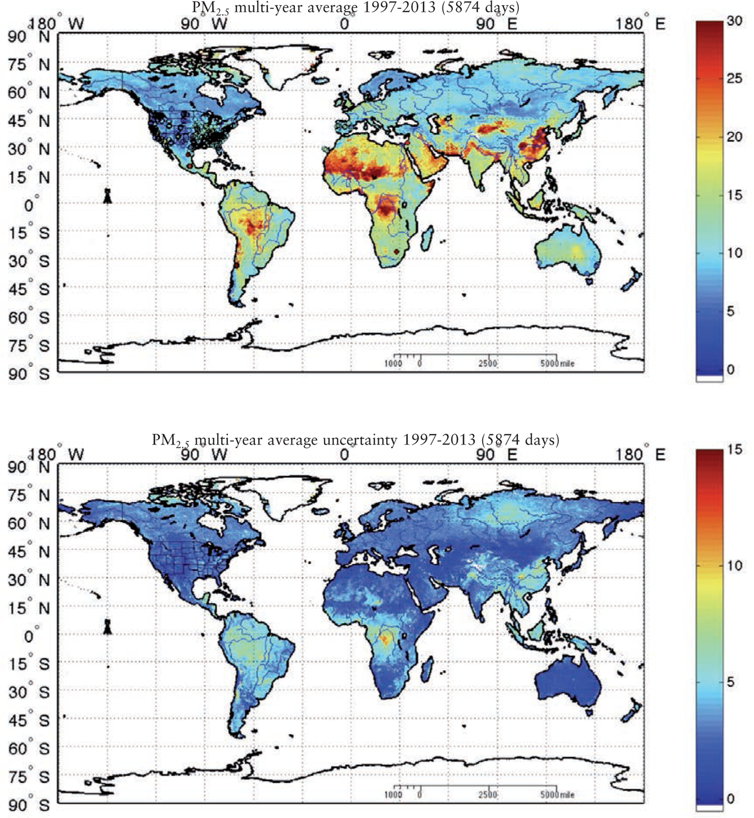
The global average of the surface PM2.5 abundance of the 5,874 daily estimates from August 1 1997 to August 31 2013 (upper panel) with the estimated uncertainty (lower panel). The surface load of PM2.5 is expressed in μg/m3 with the observations for those locations, for which we have both a machine-learning estimate of the surface PM2.5 abundance and an observation for at least one third of the 5,874, overlaid as colour-filled circles. The agreement between the machine-learning estimate and the in situ observations is well within the estimated uncertainty shown in the lower panel.
Results
Machine-learning estimates works best with a high volume of good quality training data (i.e. USA, Europe, Israel, Tasmania, a few sites in Chile and some parts of Asia). As can be seen in Fig. 2, the volume of training data has increased with time. The most significant recent data sources have come from a network of Chinese monitors. Asia is probably the most challenging region to accurately estimate PM2.5 abundance. This is due to both the magnitude of the sources and the large spatial and temporal gradients. The estimates in Asia were dramatically improved by the inclusion of the Asian monitoring sites in our training datasets. The second most challenging regions are Africa and South America due to the paucity of observations and a range of large PM2.5 sources. The inclusion of Israeli, South African, Mexican, Chilean and Brazilian monitoring sites in our training datasets did improve the quality for Africa and South America. The third most challenging regions are Australia and New Zealand. The inclusion of the excellent Tasmania network as well as Australian and New Zealand monitoring sites dramatically improved the quality of our PM2.5 abundance estimates in these countries. However, more PM2.5 monitoring stations are needed in the Arabian peninsula, Africa, the Philippines, Indonesia, India and South America.
It is worth noting that the uncertainty estimate is provided by our machine-learning approach. Just as we learnt the behaviour of the PM2.5 abundance as a function of the 30 plus parameters obtained from satellites, meteorological analyses and population density estimates, we also learnt a second quantity, namely the uncertainty of our PM2.5 abundance as a function of the same 30 plus parameters. So for Saharan Africa and the Middle East, where there are few PM2.5 monitors (apart from in Israel), the uncertainty is based objectively on how well the machine-learning algorithm was able to estimate the PM2.5 abundance for that part of the parameter space defined by the 30 plus parameters covering AOD, temperature, humidity etc. Sporadic wild-fires and biomass burning are a major source of PM2.5 in places such as sub-Saharan Africa, Amazonia, parts of Mexico, western USA, etc. These sporadic sources are not so pronounced in Fig. 7 as it represents such a long-term average as 5,874 daily estimates from August 1 1997 to August 31 2013. However, the burning in some regions is so persistent that it is evident even in the long-term average, e.g. in the Democratic Republic of Congo (marked M in Fig. 8).
Fig. 8.
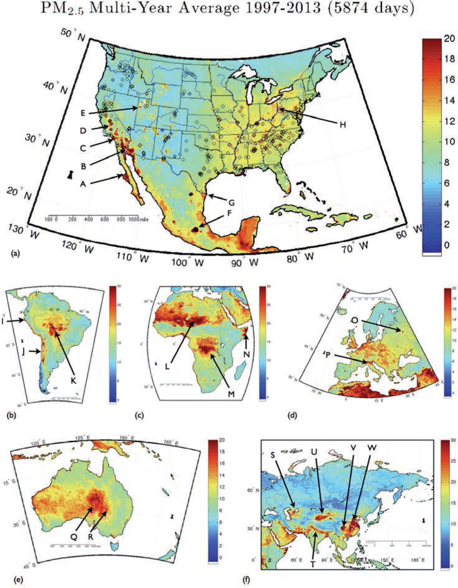
The average of the surface PM2.5 abundance of the 5,874 daily estimates from August 1, 1997 to August 31 2013 in μg/m3 for the world’s inhabited continents. Particularly high levels of PM2.5 are found in Muleg Municipality close to Guerrero Negro (A); the Sonoran Desert (B); Los Angeles (C); Central Valley in California (D); Great Salt Lake Desert, Utah (E); Mexico City (F); the Chihuahuan and the Big Bend deserts (G); Ohio River Valley (H);. Piura Desert (I); coast from Andean Altiplano Basin to Neuquen Basin (J); Amazon area, Bolivia (K); Bodelle depression in Chad (L); south of Congo River (M); coastal Somalia (N); Moscow (O); Po Valley (P); Lake Eyre (Q); Strzelecki Desert (R); Aral Sea (S) Ganges Valley (T); Taklimakan Desert (U); Sichuan Basin (V); and the region from Beijing to Guangxi in China (W).
Key features by region
The Americas –
In Fig. 8a we see that the eastern half has a higher average abundance of PM2.5than the western half of the USA with the exception of California (Herner et al., 2005). This is consistent with the overlaid EPA observations shown as colour-filled circles. The fill for the observations uses the same colour scale as the machine-learning background estimates. There are persistently high levels of PM2.5 in Mexico’s dusty and desolate Baja California Sur. The particularly high values are in Muleg Municipality close to Guerrero Negro (A). The Sonoran Desert (B), a region characterised by high average PM2.5 abundance and American dust storms (Haboobs) (Idso et al., 1972; Vasquez et al., 1998; Wilt et al., 1998), straddles the region close to the Mexico, Arizona and California borders (Brazel and Nickling, 1978; Holcombe et al., 1997). It covers an area of 311,000 km2 and is one of the hottest and dustiest parts of North America. This is clearly evident in the high 16-year average PM2.5 abundance in this region.
The persistently high PM2.5 abundance associated with Los Angeles (C) is visible. As observed by van Donkelaar et al. (2006), the regions of high population density coincide with the region of high particulate abundance. California’s heavily agricultural Central Valley (D) has a high PM2.5 load (note the good agreement of our estimates with the 16 year average observations). The EPA has designated Central Valley as a non-attainment area for the 24-hour PM2.5 National Ambient Air Quality Standards (NAAQS). The high PM2.5 abundance associated with the Great Salt Lake Desert in northern Utah (E) close to the Nevada border stands out. There is a nearby measurement “supersite” at Salt Lake City (Long et al., 2003) recording a particulate abundances consistent with our estimates.
Mexico City is known for its high levels of particulates and is clearly visible as a localised hotspot (F). Close to the Mexico/Texas border we see the elevated PM2.5 abundance associated with the Chihuahuan Desert and the Big Bend Desert (G). Dust storms in this area often impact El Paso in Texas and Ciudad Juarez in Mexico (Rivera et al., 2010, 2009; Baddock et al., 2011). The Ohio River Valley (H) encompasses several states and is home to numerous coal-fired power plants, chemical plants and industrial facilities, leading to high levels of ambient particulates (Khosah et al., 2000; Anderson et al., 2004; Yatavelli et al., 2006; Kim et al., 2007). The Ohio River Valley has a higher average abundance of PM2.5 than the rest of the East Coast. Our analysis agrees closely with the in-situ observations reported by (Yatavelli et al., 2006) for the Athens “supersite”. The Piura Desert in northern Peru (I) on the coast and western slopes of the Andes is a region of high particulate abundances. The region in South America (J) stretching from the high Andean semi-arid Altiplano basin in the North, coming down through the Salar de Uyuni Desert (the world’s largest salt flats), passing by Santiago in Chile (Koutrakis et al., 2005) and San Miguel de Tucumn, San Juan and Mendoza in Argentina and down to the Neuquen Basin in the South is characterised by a high abundance of particles from a combination of dust, salt and pollution. The southern Amazon in Bolivia and the surrounding region (K) has a lot of burning leading to persistently high particulate abundances.
Africa –
The Bodelle depression (L) is Chad’s lowest point on the Sahara’s southern edge that supplies the Amazon forest with the majority of its mineral dust (Washington and Todd, 2005; Koren et al., 2006; Washington et al., 2006a,b; Todd et al., 2007; Bouet et al., 2012). The high abundance of PM2.5 over the Bodelle is clearly visible. Typically, there are dust storms originating from the Bodelle depression around 100 days a year. Washington and Todd (2005) examined the dynamical controls of the Bodelle low-level jet features. The major source of the world’s Aeolian dust is the Sahara (Goudie and Middleton, 2001; Middleton and Goudie, 2001). The low, flat area that is Western Sahara is some of the most inhospitable and arid land on earth and a substantial dust source, clearly visible in the high abundance of PM2.5. Burning in the Democratic Republic of Congo (M) leads to high levels of particulates. Much of coastal Somalia (N) is desert characterised by high levels of particulates.
Europe –
An example of a local pollution hotspot in Europe is Moscow (O). Otherwise, the Italian Po Valley (P) has some of the highest average fine particle abundance in Europe with industrial emissions coupled with persistent fog leading to smog (Zappoli et al., 1999; Schaap et al., 2002; Putaud et al., 2004; Crosier et al., 2007).
Australia –
Lake Eyre (Q) is Australia’s largest lake and lowest point, but it usually only fills with water after heavy rains that typically occur only every three years; otherwise it consists of a salt crust. When the lake does fill, the depth is usually up to 1.5 m; once in a decade it will fill up to 4 m, after which the level falls by around 30 cm a month. When Lake Eyre has dried out, it is Australia’s largest dust source, while the PM2.5 abundance there and in its vicinity is lower than usual during the periods when it is filled with water. Just east of the Lake Eyre Basin is the Strzelecki Desert (R), another major Australian dust source. The arid region just south of the Hamersley Range in Western Australia, i.e. the Gibson Desert, Great Victoria Desert and MacDonnell Ranges, are also dusty environments with elevated average abundances of PM2.5.
Asia –
Asia has some of the highest particulate abundances anywhere on Earth. The Aral Sea (S) lying across the border of Kazakhstan and Uzbekistan is heavily polluted with major public health problems. The Ganges Valley (T) is home to 100 million people and is highly polluted. The cold Taklimakan Desert of northwest China (U) has an area of 337,000 km2 and is a major source of PM2.5, and so is the situatuion in the Sichhuan the Sichuan Basin (V) and in the western China in the region from Beijing in the North down to Guangxi in the South (W).
Discussion
A PM2.5 data product useful for human health studies needs to resolve both spatial and temporal variability. Figs. 3 and 4 show that our machine-learning approach well reproduces the shape of the probability distributions of the globally observed PM2.5 abundance. Figs. 7 and 8 show that it also reproduces the global average spatial distributions well.
A strength of this study is the daily global coverage from 1997 to the present. However, as a consequence of having a wide array of point sources, the PM2.5 abundance can contain high spatial variability on small scales. The spatial resolution of our study is 10 × 10 km (approximately 0.1° × 0.1°) determined by the spatial resolution of the MODIS collection-5 aerosol products. Spatial variability on scales smaller than 10 km is present. However, they are unresolved in our data product and there are also data gaps due to both cloud coverage and the difficulty that the standard MODIS retrieval algorithm has with retrievals over bright surfaces. MODIS collection-6 is about to be released and will help address several of these issues. This collection will have 3-km resolution and greater Deep Blue data coverage. Collection-6 will include various refinements, such as extended coverage to vegetated and bright land surfaces, improved cloud screening, surface reflectance and aerosol microphysical models. In addition, any satellite instrument has a finite life and both MODIS satellites (Terra and Aqua) are aging. We hope data continuity will be provided by the recently launched Visible Infrared Imaging Radiometer Suite (VIIRS) on the Suomi National Polar-orbiting Partnership weather satellite. When data quality from VIIRS becomes acceptable those data can also be used. Although to our knowledge, we have used more training data than any other studies of PM2.5 estimation, there are yet certain parts of the world from where we are still collecting such data. This lack of uniformity in training data may cause some inconsistency in data product quality. However, as we make progress in acquiring more ground PM2.5 data from different parts of the world with missing information, the quality of our dataset will be improved for those parts of the world as well.
Conclusions
A new approach to use ground-based observations of PM together with a suite of remote sensing and meteorological data products training a machine-learning algorithm to estimate the daily distributions of PM2.5 has been demonstrated. This new PM2.5 daily global data product reproduces global observations and spans an unprecedented 16 years from 1997 to the present. The correlation coefficient for each of the five training datasets is 0.96 or greater and the correlation coefficient for each of the independent validation datasets is 0.52 or greater. The quality varies slightly with satellite, with the best fits obtained from Terra data, followed by Aqua and SeaWIFS. In all cases the shape of PM2.5 data product reproduces the observations between the 25th and 75th quantiles. The machine-learning PM2.5 data product is useful for human health studies as it resolves both spatial and temporal variability.
Acknowledgments
It is a pleasure to acknowledge the Institute for Integrative Health, the University of Texas at Dallas, DoD TATRC for Award W81XWH-11-2-0165, Grant Number R21ES019713 from the National Institute of Environmental Health Sciences and NASA for research funding through the award NNX11AL18G. The content is solely the responsibility of the authors and does not necessarily represent the official views of the funding agencies. It is a pleasure to acknowledge the environment agencies of Albania, Australia, Austria, Azores Islands, Belarus, Belgium, Brazil, Canada, Canary Islands, Chile, China, Croatia, Cyprus, Czech Republic, Denmark, Estonia, Finland, France, Germany, Greece, Hong Kong, Hungary, Iceland, Iceland, India, Ireland, Israel, Italy, Japan, Latvia, Lithuania, Madeira Islands, Malaysia, Mexico, Mongolia, New Zealand, Netherlands, Norway, Peru, Poland, Portugal, Russia, Singapore, Slovakia, South Africa, South Korea, Spain, Sweden, Taiwan, Thailand, United Kingdom, United States and Vietnam for the use of their PM2.5 observations.
References
- Andersen ZJ, 2012. Health effects of long-term exposure to air pollution: an overview of major respiratory and cardiovascular diseases and diabetes. Chem Ind Chem Eng Q 18, 617–622. [Google Scholar]
- Andersen ZJ, Raaschou-Nielsen O, Ketzel M, Jensen SS, Hvidberg M, Loft S, Tjonneland A, Overvad K, Sorensen M, 2012. Diabetes incidence and long-term exposure to air pollution a cohort study. Diabetes Care 35, 92–98. [DOI] [PMC free article] [PubMed] [Google Scholar]
- Anderson HR, Butland BK, van Donkelaar A, Brauer M, Strachan DP, Clayton T, van Dingenen R, Amann M, Brunekreef B, Cohen A, et al. , 2012. Satellite-based estimates of ambient air pollution and global variations in childhood asthma prevalence. Environ Health Perspect 120, 1333–1339. [DOI] [PMC free article] [PubMed] [Google Scholar]
- Anderson RR, Martello DV, White CM, Crist KC, John K, Modey WK, Eatough DJ, 2004. The regional nature of PM2.5 episodes in the upper Ohio River Valley. J Air Waste Manag Assoc 54, 971–984. [DOI] [PubMed] [Google Scholar]
- Araujo JA, 2011. Particulate air pollution, systemic oxidative stress, inflammation, and atherosclerosis. Air Qual Atmos Health 4, 79–93. [DOI] [PMC free article] [PubMed] [Google Scholar]
- Araujo JA, Barajas B, Kleinman M, Wang X, Bennett BJ, Gong KW, Navab M, Harkema J, Sioutas C, Lusis AJ, Nel AE, 2008. Ambient particulate pollutants in the ultrafine range promote early atherosclerosis and systemic oxidative stress. Circ Res 102, 589–596. [DOI] [PMC free article] [PubMed] [Google Scholar]
- Ayala A, Brauer M, Mauderly JL, Samet JM, 2012. Air pollutants and sources associated with health effects. Air Qual Atmos Health 5, 151–167. [Google Scholar]
- Baccarelli A, Barretta F, Dou C, Zhang X, McCracken JP, Diaz A, Bertazzi PA, Schwartz J, Wang S, Hou L, 2011. Effects of particulate air pollution on blood pressure in a highly exposed population in Beijing, China: a repeated-measure study. Environ Health 10, 108. [DOI] [PMC free article] [PubMed] [Google Scholar]
- Baccarelli A, Tarantini L, Bonzini M, Apostoli P, Pegoraro V, Bollati V, Marinelli B, Cantone L, Rizzo G, Hou L, et al. , 2008. Effects of particulate matter on genomic DNA methylation content and inos promoter methylation. Epidemiology 19, S259–S260. [DOI] [PMC free article] [PubMed] [Google Scholar]
- Baccarelli A, Wright RO, Bollati V, Tarantini L, Litonjua AA, Suh HH, Zanobetti A, Sparrow D, Vokonas PS, Schwartz J, 2009. Rapid DNA methylation changes after exposure to traffic particles. Am J Respir Crit Care Med 179, 572–578. [DOI] [PMC free article] [PubMed] [Google Scholar]
- Baddock MC, Gill TE, Bullard JE, Dominguez Acosta M, Rivera NIR, 2011. Geomorphology of the Chihuahuan Desert based on potential dust emissions. J Maps 2011, 249–259. [Google Scholar]
- Ballester F, Medina S, Boldo E, Goodman P, Neuberger M, Iniguez C, Kunzli N, Apheis N, 2008. Reducing ambient levels of fine particulates could substantially improve health: a mortality impact assessment for 26 European cities. J Epidemiol Community Health 62, 98–105. [DOI] [PubMed] [Google Scholar]
- Block ML, Calderon-Garciduenas L, 2009. Air pollution: mechanisms of neuroinflammation and CNS disease. Trends Neurosci 32, 506–516. [DOI] [PMC free article] [PubMed] [Google Scholar]
- Boldo E, Linares C, Lumbreras J, Borge R, Narros A, Garcia-Perez J, Fernandez-Navarro P, Perez-Gomez B, Aragones N, Ramis R, et al. , 2011. Health impact assessment of a reduction in ambient PM2.5 levels in Spain. Environ Int 37, 342–348. [DOI] [PubMed] [Google Scholar]
- Boldo E, Medina S, LeTertre A, Hurley F, Muecke HG, Ballester F, Aguilera I, Eilstein D, Apheis G, 2006. Apheis: health impact assessment of long-term exposure to PM2.5 in 23 European cities. Eur J Epidemiol 21, 449–458. [DOI] [PubMed] [Google Scholar]
- Bouet C, Cautenet G, Bergametti G, Marticorena B, Todd MC, Washington R, 2012. Sensitivity of desert dust emissions to model horizontal grid spacing during the bodele dust experiment 2005. Atmos Environ 50, 377–380. [Google Scholar]
- Brauer M, Amann M, Burnett RT, Cohen A, Dentener F, Ezzati M, Henderson SB, Krzyzanowski M, Martin RV, Van Dingenen R, et al. , 2012. Exposure assessment for estimation of the global burden of disease attributable to outdoor air pollution. Environ Sci Technol 46, 652–660. [DOI] [PMC free article] [PubMed] [Google Scholar]
- Brazel AJ, Nickling WG, 1987. Dust storms and their relation to moisture in the Sonoran-Mojave desert region of the Southwestern United States. J Environ Manage 24, 279–291. [Google Scholar]
- Brook RD, 2008. Cardiovascular effects of air pollution. Clin Sci (Lond) 115, 175–187. [DOI] [PubMed] [Google Scholar]
- Brook RD, Bard RL, Kaplan MJ, Yalavarthi S, Morishita M, Dvonch JT, Wang L, Yang H-Y, Spino C, Mukherjee B, et al. , 2013. The effect of acute exposure to coarse particulate matter air pollution in a rural location on circulating endothelial progenitor cells: results from a randomized controlled study. Inhal Toxicol 25, 587–592. [DOI] [PMC free article] [PubMed] [Google Scholar]
- Brook RD, Rajagopalan S, 2009. Particulate matter, air pollution, and blood pressure. J Am Soc Hypertens 3, 332–350. [DOI] [PubMed] [Google Scholar]
- Brook RD, Rajagopalan S, 2012. Can what you breathe trigger a stroke within hours? Arch Intern Med 172, 235–236. [DOI] [PubMed] [Google Scholar]
- Brook RD, Rajagopalan S, Pope C, Arden I, Brook JR, Bhatnagar A, Diez-Roux AV, Holguin F, Hong Y, Luepker RV, et al. , 2010a. Particulate matter air pollution and cardiovascular disease an update to the scientific statement from the American Heart Association. Circulation 121, 2331–2378. [DOI] [PubMed] [Google Scholar]
- Brook RD, Xu X, Bard RL, Dvonch JT, Morishita M, Kaciroti N, Sun Q, Harkema J, Rajagopalan S, 2013. Reduced metabolic insulin sensitivity following sub-acute exposures to low levels of ambient fine particulate matter air pollution. Sci Total Environ 448, 66–71. [DOI] [PMC free article] [PubMed] [Google Scholar]
- Byun HM, Panni T, Motta V, Hou L, Nordio F, Apostoli P, Bertazzi PA, Baccarelli AA, 2013. Effects of airborne pollutants on mitochondrial dna methylation. Part Fibre Toxicol 10, 18. [DOI] [PMC free article] [PubMed] [Google Scholar]
- Cesaroni G, Forastiere F, Stafoggia M, Andersen ZJ, Badaloni C, Beelen R, Caracciolo B, de Faire U, Erbel R, Eriksen KT, et al. , 2014. Long term exposure to ambient air pollution and incidence of acute coronary events: prospective cohort study and meta-analysis in 11 European cohorts from the ESCAPE Project. BMJ 348, 12. [DOI] [PMC free article] [PubMed] [Google Scholar]
- Chambers JM, Cleveland WS, Kleiner B, Tukey PA, 1983. Graphical methods for data analysis, Wadsworth International Group, Belmont, Calif. [Google Scholar]
- Chen JC, Schwartz J, 2009. Neurobehavioral effects of ambient air pollution on cognitive performance in us adults. Neurotoxicology 30, 231–239. [DOI] [PubMed] [Google Scholar]
- Choi YS, Ho CH, Chen D, Noh YH, Song CK, 2008. Spectral analysis of weekly variation in PM10 mass concentration and meteorological conditions over China. Atmos Environ 42, 655–666. [Google Scholar]
- Crosier J, Allan JD, Coe H, Bower KN, Formenti P, Williams PI, 2007. Chemical composition of summertime aerosol in the Po Valley (Italy), Northern Adriatic and Black Sea. Q J Roy Meteor Soc 133, 61–75. [Google Scholar]
- Crouse DL, Peters PA, van Donkelaar A, Goldberg MS, Villeneuve PJ, Brion O, Khan S, Atari DO, Jerrett M, Pope C, et al. , 2012. Risk of non accidental and cardiovascular mortality in relation to long-term exposure to low concentrations of fine particulate matter: A Canadian national-level cohort study. Environ Health Perspect 120, 708–714. [DOI] [PMC free article] [PubMed] [Google Scholar]
- Dadvand P, Parker J, Bell ML, Bonzini M, Brauer M, Darrow LA, Gehring U, Glinianaia SV, Gouveia N, Ha EH, et al. , 2013. Maternal exposure to particulate air pollution and term birth weight: A multi-country evaluation of effect and heterogeneity. Environ Health Perspect 121, 367–373. [DOI] [PMC free article] [PubMed] [Google Scholar]
- Dales R, Burnett RT, Smith-Doiron M, Stieb DM, Brook JR, 2004. Air pollution and sudden infant death syndrome. Pediatrics 113, E628–E631. [DOI] [PubMed] [Google Scholar]
- De Prins S, Koppen G, Jacobs G, Dons E, Van de Mieroop E, Nelen V, Fierens F, Panis LI, De Boever P, Cox B, et al. , 2013. Influence of ambient air pollution on global DNA methylation in healthy adults: a seasonal follow-up. Environ Int 59, 418–424. [DOI] [PubMed] [Google Scholar]
- Dockery DW, Pope CA, Xu XP, Spengler JD, Ware JH, Fay ME, Ferris BG, Speizer FE, 1993. An association between air-pollution and mortality in 6 United States cities. N Engl J Med 329, 1753–1759. [DOI] [PubMed] [Google Scholar]
- Engel-Cox JA, Hoff RM, Haymet ADJ, 2004. Recommendations on the use of satellite remote-sensing data for urban air quality. J Air Waste Manag Assoc 54, 1360–1371. [DOI] [PubMed] [Google Scholar]
- Engel-Cox JA, Hoff RM, Rogers R, Dimmick F, Rush AC, Szykman JJ, Al-Saadi J, Chu DA, Zell ER, 2006. Integrating LIDAR and satellite optical depth with ambient monitoring for 3-dimensional particulate characterization. Atmos Environ 40, 8056–8067. [Google Scholar]
- Engel-Cox JA, Holloman CH, Coutant BW, Hoff RM, 2004. Qualitative and quantitative evaluation of MODIS satellite sensor data for regional and urban scale air quality. Atmos Environ 38, 2495–2509. [Google Scholar]
- Engel-Cox J, Oanh NTK, van Donkelaar A, Martin RV, Zell E, 2013. Toward the next generation of air quality monitoring: particulate matter. Atmos Environ 80, 584–590. [Google Scholar]
- Farhat SCL, Silva CA, Orione MAM, Campos LMA, Sallum AME, Braga ALF, 2011. Air pollution in autoimmune rheumatic diseases: a review. Autoimmun Rev 11, 14–21. [DOI] [PubMed] [Google Scholar]
- Fowlkes EB, 1987. A folio of distributions: a collection of theoretical quantile-quantile plots. New York: Marcel Dekker, 540 pp. [Google Scholar]
- Franklin M, Zeka A, Schwartz J, 2007. Association between PM2.5 and all-cause and specific-cause mortality in 27 US communities. J Expo Sci Environ Epidemiol 17, 279–287. [DOI] [PubMed] [Google Scholar]
- Ginoux P, Torres O, 2003. Empirical TOMS index for dust aerosol: applications to model validation and source characterization. J Geophys Res Atmos 108, 4534. [Google Scholar]
- Glinianaia SV, Rankin J, Bell R, Pless-Mulloli T, Howel D, 2004. Does particulate air pollution contribute to infant death? A systematic review. Environ Health Perspect 112, 1365–1370. [DOI] [PMC free article] [PubMed] [Google Scholar]
- Goudie AS, Middleton NJ, 2001. Saharan dust storms: nature and consequences. Earth-Sci Rev 56, 179–204. [Google Scholar]
- Herner JD, Aw J, Gao O, Chang DP, Kleeman MJ, 2005. Size and composition distribution of airborne particulate matter in northern California: I-particulate mass, carbon, and water-soluble ions. J Air Waste Manage Assoc 55, 30–51. [DOI] [PubMed] [Google Scholar]
- Hoff RM, Christopher SA, 2009. Remote sensing of particulate pollution from space: have we reached the promised land? J Air Waste Manage Assoc 59, 642–644. [PubMed] [Google Scholar]
- Hoffmann B, Moebus S, Dragano N, Stang A, Moehlenkamp S, Schmermund A, Memmesheimer M, Broecker-Preuss M, Mann K, Erbel R, et al. , 2009. Chronic residential exposure to particulate matter air pollution and systemic inflammatory markers. Environ Health Perspect 117, 1302–1308. [DOI] [PMC free article] [PubMed] [Google Scholar]
- Holcombe TL, Ley T, Gillette DA, 1997. Effects of prior precipitation and source area characteristics on threshold wind velocities for blowing dust episodes, Sonoran Desert 1948–78. J Appl Meteorol 36, 1160–1175. [Google Scholar]
- Hou L, Wang S, Dou C, Zhang X, Yu Y, Zheng Y, Avula U, Hoxha M, Diaz A, McCracken J, et al. , 2012. Air pollution exposure and telomere length in highly exposed subjects in Beijing, China: a repeated-measure study. Environ Int 48, 71–77. [DOI] [PMC free article] [PubMed] [Google Scholar]
- Hou L, Zhang X, Dioni L, Barretta F, Dou C, Zheng Y, Hoxha M, Bertazzi PA, Schwartz J, Wu S, et al. , 2013. Inhalable particulate matter and mitochondrial DNA copy number in highly exposed individuals in Beijing, China: a repeated-measure study. Part Fibre Toxicol 10. [DOI] [PMC free article] [PubMed] [Google Scholar]
- Hou L, Zhu ZZ, Zhang X, Nordio F, Bonzini M, Schwartz J, Hoxha M, Dioni L, Marinelli B, Pegoraro V, et al. , 2010. Airborne particulate matter and mitochondrial damage: a cross-sectional study. Environ Health 9. [DOI] [PMC free article] [PubMed] [Google Scholar]
- Hsu NC, Tsay SC, King MD, Herman JR, 2004. Aerosol properties over bright-reflecting source regions. IEEE Trans Geosci Remote Sens 42, 557–569. [Google Scholar]
- Hsu NC, Tsay SC, King MD, Herman JR, 2006. Deep blue retrievals of Asian aerosol properties during ACE-Asia. IEEE Trans Geosci Remote Sens 44, 3180–3195. [Google Scholar]
- Hyer EJ, Reid JS, Zhang J, 2011. An over-land aerosol optical depth data set for data assimilation by filtering, correction, and aggregation of MODIS collection 5 optical depth retrievals. Atmos Meas Tech 4, 379–408. [Google Scholar]
- Hystad P, Demers PA, Johnson KC, Brook J, van Donkelaar A, Lamsal L, Martin R, Brauer M, 2012. Spatiotemporal air pollution exposure assessment for a Canadian population-based lung cancer case-control study. Environ Health 11, 22. [DOI] [PMC free article] [PubMed] [Google Scholar]
- Hystad P, Setton E, Cervantes A, Poplawski K, Deschenes S, Brauer M, van Donkelaar A, Lamsal L, Martin R, Jerrett M, et al. , 2011. Creating national air pollution models for population exposure assessment in Canada. Environ Health Perspect 119, 1123–1129. [DOI] [PMC free article] [PubMed] [Google Scholar]
- Hystad P, Setton E, Cervantes A, Poplawski K, Deschenes S, Tomlins M, Martin R, Van Donkelaar A, 2009. Feasibility of a Canadian land use regression model for PM2.5 exposure assessment. Epidemiology 20, S191. [Google Scholar]
- Idso SB, Ingram RS, Pritchar JM, 1972. An American haboob. B Am Meteorol Soc 53, 930–935. [Google Scholar]
- Ji H, Hershey GKK, 2012. Genetic and epigenetic influence on the response to environmental particulate matter. Am J Clin Exp Immunol 129, 33–41. [DOI] [PMC free article] [PubMed] [Google Scholar]
- Kaufman J, 2011. An update on the multiethnic study of atherosclerosis and air pollution. Epidemiology 22, S226–S227. [Google Scholar]
- Khosah RP, McManus TJ, Feeley TJ, 2000. Ambient fine particulate (PM2.5) monitoring research for the upper Ohio River Valley project. Abstr Pap Am Chem Soc 219, 45–49. [Google Scholar]
- Kim M, Deshpande SR, Crist KC, 2007. Source apportionment of fine particulate matter (PM2.5) at a rural Ohio River Valley site. Atmos Environ 41, 9231–9243. [Google Scholar]
- Koren I, Kaufman YJ, Washington R, Todd MC, Rudich Y, Martins JV, Rosenfeld D, 2006. The bodele depression: a single spot in the Sahara that provides most of the mineral dust to the Amazon forest. Environ Res Lett 1, 4345–4372. [Google Scholar]
- Koutrakis P, Sax SN, Sarnat JA, Coull B, Demokritou P, Oyola P, Garcia J, Gramsch E, 2005. Analysis of PM10, PM2.5, and PM2.5 −10 concentrations in Santiago, Chile, from 1989 to 2001. J Air Waste Manag Assoc 55, 342–351. [DOI] [PubMed] [Google Scholar]
- Kreyling WG, Semmler-Behnke M, Moller W, 2006. Ultrafine particle-lung interactions: does size matter? J Aerosol Med 19, 74–83. [DOI] [PubMed] [Google Scholar]
- Kumar N, Chu AD, Foster AD, Peters T, Willis R, 2011. Satellite remote sensing for developing time and space resolved estimates of ambient particulate in Cleveland, OH. Aerosol Sci Technol 45, 1090–1108. [DOI] [PMC free article] [PubMed] [Google Scholar]
- Lary DJ, Remer LA, MacNeill D, Roscoe B, Paradise S, 2009. Machine learning and bias correction of MODIS aerosol optical depth. IEEE Trans Geosci Remote Sens 6, 694–698. [Google Scholar]
- Lary DJ, Woolf S, Faruque F, LePage J, 2014. Holistics 3.0 for Health. ISPRS Int J Geo-Inf 3, 1023–1038. [Google Scholar]
- Lee HJ, Liu Y, Coull BA, Schwartz J, Koutrakis P, 2011a. A novel calibration approach of MODIS AOD data to predict PM2.5 concentrations. Atmos Chem Phys 11, 7991–8002. [Google Scholar]
- Lee HJ, Liu Y, Coull B, Schwartz Koutrakis P, 2011b. PM2.5 prediction modeling using MODIS AOD and its implications for health effect studies. Epidemiology 22, S215. [Google Scholar]
- Lipfert FW, Zhang J, Wyzga RE, 2000. Infant mortality and air pollution: a comprehensive analysis of US data for 1990. J Air Waste Manag Assoc 50, 1350–1366. [DOI] [PubMed] [Google Scholar]
- Liu Y, Chen D, Kahn RA, He K, 2009a. Review of the applications of multiangle imaging spectroradiometer to air quality research. Sci China Ser D Earth Sci 52, 132–144. [Google Scholar]
- Liu Y, Franklin M, Kahn R, Koutrakis P, 2007a. Using aerosol optical thickness to predict ground-level PM2.5 concentrations in the St. Louis area: a comparison between MISR and MODIS. Remote Sens Environ 107, 33–44. [Google Scholar]
- Liu Y, He K, Li S, Wang Z, Christiani DC, Koutrakis P, 2012. A statistical model to evaluate the effectiveness of PM2.5 emissions control during the Beijing 2008 olympic games. Environ Int 44, 100–105. [DOI] [PubMed] [Google Scholar]
- Liu YJ, Harrison RM, 2011. Properties of coarse particles in the atmosphere of the United Kingdom. Atmos Environ 45, 3267–3276. [Google Scholar]
- Liu Y, Kahn RA, Chaloulakou A, Koutrakis P, 2009b. Analysis of the impact of the forest fires in august 2007 on air quality of Athens using multi-sensor aerosol remote sensing data, meteorology and surface observations. Atmos Environ 43, 3310–3318. [Google Scholar]
- Liu Y, Koutrakis P, Kahn R, 2007b. Estimating fine particulate matter component concentrations and size distributions using satellite-retrieved fractional aerosol optical depth: part 1 - method development. J Air Waste Manag Assoc 57, 1351–1359. [DOI] [PubMed] [Google Scholar]
- Liu Y, Koutrakis P, Kahn R, Turquety S, Yantosca RM, 2007c. Estimating fine particulate matter component concentrations and size distributions using satellite-retrieved fractional aerosol optical depth: part 2 - a case study. J Air Waste Manag Assoc 57, 1360–1369. [DOI] [PubMed] [Google Scholar]
- Liu Y, Paciorek CJ, Koutrakis P, 2009. Estimating regional spatial and temporal variability of PM2.5 concentrations using satellite data, meteorology, and land use information. Environ Health Perspect 117, 886–892. [DOI] [PMC free article] [PubMed] [Google Scholar]
- Liu Y, Paciorek C, Koutrakis P, 2008. Estimating daily pm2.5 exposure in Massachusetts with satellite aerosol remote sensing data, meteorological, and land use information. Epidemiology 19, S116. [Google Scholar]
- Liu Y, Park RJ, Jacob DJ, Li QB, Kilaru V, Sarnat JA, 2004. Mapping annual mean ground-level PM2.5 concentrations using multiangle imaging spectroradiometer aerosol optical thickness over the contiguous United States. J Geophys Res Atmos 109, D22206. [Google Scholar]
- Liu Y, Sarnat JA, Kilaru A, Jacob DJ, Koutrakis P, 2005. Estimating ground-level PM2.5 in the Eastern United States using satellite remote sensing. Environ Sci Technol 39, 3269–3278. [DOI] [PubMed] [Google Scholar]
- Long RW, Eatough NL, Mangelson NF, Thompson W, Fiet K, Smith S, Smith R, Eatough DJ, Pope CA, Wilson WE, 2003. The measurement of PM2.5, including semi-volatile components, in the EMPACT program: results from the Salt Lake City Study. Atmos Environ 37, 4407–4417. [Google Scholar]
- Lyamani H, Olmo FJ, Alcantara A, Alados-Arboledas L, 2006. Atmospheric aerosols during the 2003 heat wave in southeastern Spain I: spectral optical depth. Atmos Environ 40, 6453–6464. [Google Scholar]
- Madrigano J, Baccarelli A, Mittleman MA, Wright RO, Sparrow D, Vokonas PS, Tarantini L, Schwartz J, 2011. Prolonged exposure to particulate pollution, genes associated with glutathione pathways, and DNA methylation in a cohort of older men. Environ Health Perspect 119, 977–982. [DOI] [PMC free article] [PubMed] [Google Scholar]
- Maheswaran R, Pearson T, Smeeton NC, Beevers SD, Campbell MJ, Wolfe CD, 2010. Impact of outdoor air pollution on survival after stroke population-based cohort study. Stroke 41, 869–877. [DOI] [PubMed] [Google Scholar]
- Maheswaran R, Pearson T, Smeeton NC, Beevers SD, Campbell MJ, Wolfe CD, 2012. Outdoor air pollution and incidence of ischemic and hemorrhagic stroke a small-area level ecological study. Stroke 43, 22–27. [DOI] [PubMed] [Google Scholar]
- Martin RV, 2008. Satellite remote sensing of surface air quality. Atmos Environ 42, 7823–7843. [Google Scholar]
- Melin F, Zibordi G, Carlund T, Holben BN, Stefan S, 2013. Validation of SeaWiFS and MODIS Aqua/Terra aerosol products in coastal regions of European marginal seas. Oceanologia 55, 27–51. [Google Scholar]
- Middleton NJ, Goudie AS, 2001. Saharan dust: sources and trajectories. Trans Inst Br Geogr 26, 165–181. [Google Scholar]
- Natunen A, Arola A, Mielonen T, Huttunen J, Komppula M, Lehtinen KEJ, 2010. A multi-year comparison of PM2.5 and AOD for the Helsinki region. Boreal Environ Res 15, 544–552. [Google Scholar]
- Paciorek CJ, Liu Y, 2009. Limitations of remotely sensed aerosol as a spatial proxy for fine particulate matter. Environ Health Perspect 117, 904–909. [DOI] [PMC free article] [PubMed] [Google Scholar]
- Paciorek CJ, Liu Y, 2012. Assessment and statistical modeling of the relationship between remotely sensed aerosol optical depth and PM2.5 in the Eastern United States. Res Rep Health Eff Inst 167. [PubMed] [Google Scholar]
- Paciorek CJ, Liu Y, Moreno-Macias H, Kondragunta S, 2008. Spatiotemporal associations between GOES aerosol optical depth retrievals and ground-level PM2.5. Environ Sci Technol 42, 5800–5806. [DOI] [PubMed] [Google Scholar]
- Patel MM, Miller RL, 2009. Rapid DNA Methylation changes after exposure to traffic particles: the issue of spatio-temporal factors. Am J Respir Crit Care Med 180, 1030–1030. [DOI] [PubMed] [Google Scholar]
- Pearson JF, Bachireddy C, Shyamprasad S, Goldfine AB, Brownstein JS, 2010. Association between fine particulate matter and diabetes prevalence in the US. Diabetes Care 33, 2196–2201. [DOI] [PMC free article] [PubMed] [Google Scholar]
- Pelletier B, Santer R, Vidot J, 2007. Retrieving of particulate matter from optical measurements: a semiparametric approach. J Geophys Res Atmos 112, D06208. [Google Scholar]
- Pope C, Arden I, Brook RD, Burnett RT, Dockery DW, 2011. How is cardiovascular disease mortality risk affected by duration and intensity of fine particulate matter exposure? An integration of the epidemiologic evidence. Air Qual Atmos Health 4, 5–14. [Google Scholar]
- Pope C, Arden I, Burnett RT, Krewski D, Jerrett M, Shi Y, Calle EE, Thun MJ, 2009. Cardiovascular mortality and exposure to airborne fine particulate matter and cigarette smoke shape of the exposure-response relationship. Circulation 120, 941–948. [DOI] [PubMed] [Google Scholar]
- Pope C, Dockery DW, 2006. Health effects of fine particulate air pollution: lines that connect. J Air Waste Manag Assoc 56, 709–742. [DOI] [PubMed] [Google Scholar]
- Prospero JM, 2003. Global dust transport over the oceans: the link to climate. Geochim Cosmochim Acta 67, A384–A384. [Google Scholar]
- Putaud JP, Raes F, Van Dingenen R, Bruggemann E, Facchini MC, Decesari S, Fuzzi S, Gehrig R, Huglin C, Laj P, et al. , 2004. European aerosol phenomenology-2: Chemical characteristics of particulate matter at kerbside, urban, rural and background sites in Europe. Atmos Environ 38, 2579–2595. [Google Scholar]
- Rajeev K, Parameswaran K, Nair SK, Meenu S, 2008. Observational evidence for the radiative impact of Indonesian smoke in modulating the sea surface temperature of the equatorial Indian Ocean. J Geophys Res Atmos 113, D17201. [Google Scholar]
- Reid JS, Hyer EJ, Johnson RS, Holben BN, Yokelson RJ, Zhang J, Campbell JR, Christopher SA, Girolamo LD, Giglio L, et al. , 2013. Observing and understanding the southeast Asian aerosol system by remote sensing: an initial review and analysis for the seven southeast Asian studies (7seas) program. Atmos Res 122, 403–468. [Google Scholar]
- Remer LA, Kleidman RG, Levy RC, Kaufman YJ, Tanre D, Mattoo S, Martins JV, Ichoku C, Koren I, Yu H, et al. , 2008. Global aerosol climatology from the MODIS satellite sensors. J Geophys Res Atmos 113, D14S07. [Google Scholar]
- Rienecker MM, Suarez MJ, Gelaro R, Todling R, Bacmeister J, Liu E, Bosilovich MG, Schubert SD, Takacs L, Kim GK, et al. , 2011. Merra: nasa’s modern-era retrospective analysis for research and applications. J Clim 24, 3624–3648. [DOI] [PMC free article] [PubMed] [Google Scholar]
- Rivera NIR, Gill TE, Bleiweiss MP, Hand JL, 2010. Source characteristics of hazardous Chihuahuan Desert dust outbreaks. Atmos Environ 44, 2457–2468. [Google Scholar]
- Rivera NIR, Gill TE, Gebhart KA, Hand JL, Bleiweiss MP, Fitzgerald RM, 2009. Wind modeling of Chihuahuan Desert dust outbreaks. Atmos Environ 43, 347–354. [Google Scholar]
- Ruckerl R, Schneider A, Breitner S, Cyrys J, Peters A, 2011. Health effects of particulate air pollution: a review of epidemiological evidence. Inhal Toxicol 23, 555–592. [DOI] [PubMed] [Google Scholar]
- Salam MT, Byun HM, Lurmann F, Breton CV, Wang X, Eckel SP, Gilliland FD, 2012. Genetic and epigenetic variations in inducible nitric oxide synthase promoter, particulate pollution, and exhaled nitric oxide levels in children. J Allergy Clin Immunol 129, 232–239. [DOI] [PMC free article] [PubMed] [Google Scholar]
- Salam MT, Millstein J, Li YF, Lurmann FW, Margolis HG, Gilliland FD, 2005. Birth outcomes and prenatal exposure to ozone, carbon monoxide, and particulate matter: results from the children’s health study. Environ Health Perspect 113, 1638–1644. [DOI] [PMC free article] [PubMed] [Google Scholar]
- Sayer AM, Hsu NC, Bettenhausen C, Jeong MJ, 2013. Validation and uncertainty estimates for MODIS collection 6 “deep blue” aerosol data. J Geophys Res Atmos 118, 7864–7872. [Google Scholar]
- Schaap M, Apituley A, Timmermans RMA, Koelemeijer RBA, de Leeuw G, 2009. Exploring the relation between aerosol optical depth and PM2.5 at Cabauw, the Netherlands. Atmos Chem Phy 9, 909–925. [Google Scholar]
- Schaap M, Muller K, ten Brink HM, 2002. Constructing the European aerosol nitrate concentration field from quality analysed data. Atmos Environ 36, 1323–1335. [Google Scholar]
- Shi Y, Zhang J, Reid JS, Hyer EJ, Hsu NC, 2012. Critical evaluation of the MODIS deep blue aerosol optical depth product for data assimilation over North Africa. Atmos Measure Tech Discuss 5, 7815–7865. [Google Scholar]
- Slama R, Darrow L, Parker J, Woodruff TJ, Strickland M, Nieuwenhuijsen M, Glinianaia S, Hoggatt KJ, Kannan S, Hurley F, et al. , 2008. Meeting report: atmospheric pollution and human reproduction. Environ Health Perspect 116, 791–798. [DOI] [PMC free article] [PubMed] [Google Scholar]
- Sunderman FW, 2001. Review: nasal toxicity, carcinogenicity, and olfactory uptake of metals. Ann Clin Lab Sci 31, 3–24. [PubMed] [Google Scholar]
- Tarantini L, Bonzini M, Apostoli P, Pegoraro V, Bollati V, Marinelli B, Cantone L, Rizzo G, Hou L, Schwartz J, et al. 2009. Effects of particulate matter on genomic dna methylation content and inos promoter methylation. Environ Health Perspect 117, 217–222. [DOI] [PMC free article] [PubMed] [Google Scholar]
- Taylor K, 2001. Summarizing multiple aspects of model performance in a single diagram. J Geophys Res 106, 7183–7192. [Google Scholar]
- Tian D, Wang Y, Bergin M, Hu Y, Liu Y, Russell AG, 2008. Air quality impacts from prescribed forest fires under different management practices. Environ Sci Technol 42, 2767–2772. [DOI] [PubMed] [Google Scholar]
- Todd MC, Washington R, Martins JV, Dubovik O, Lizcano G, M’Bainayel S, Engelstaedter S, 2007. Mineral dust emission from the Bodele depression, northern Chad, during Bodex 2005. J Geophys Res Atmos 112, D06207. [Google Scholar]
- van de Kassteele J, Koelemeijer RBA, Dekkers ALM, Schaap M, Homan CD, Stein A, 2006. Statistical mapping of PM10 concentrations over Western Europe using secondary information from dispersion modeling and MODIS satellite observations. Stoch Environ Res Risk Assess 21, 183–194. [Google Scholar]
- van Donkelaar A, Martin RV, Brauer M, Kahn R, Levy R, Verduzco C, Villeneuve PJ, 2010. Global estimates of ambient fine particulate matter concentrations from satellite-based aerosol optical depth: Development and application. Environ Health Perspect 118, 847–855. [DOI] [PMC free article] [PubMed] [Google Scholar]
- van Donkelaar A, Martin RV, Levy RC, da Silva AM, Krzyzanowski M, Chubarova NE, Semutnikova E, Cohen AJ, 2011. Satellite-based estimates of ground-level fine particulate matter during extreme events: a case study of the Moscow fires in 2010. Atmos Environ 45, 6225–6232. [Google Scholar]
- van Donkelaar A, Martin RV, Park RJ, 2006. Estimating ground-level PM2.5 using aerosol optical depth determined from satellite remote sensing. J Geophys Res 111, D21201. [Google Scholar]
- van Donkelaar A, Martin R, Verduzco C, Brauer M, Kahn R, Levy R, Villeneuve P, 2010. A hybrid approach for predicting PM2.5 exposure response. Environ Health Perspect 118, A425. [DOI] [PMC free article] [PubMed] [Google Scholar]
- Vasquez HR, Fausett J, Sipple S, Estle WT, Haro JA, Wojcik W, Berkovitz R, Sturm D, Cushmeer N, Jamison A, et al. , 1998. A South-Central Arizona Haboob - the 28 July 1994 wind and dust storm. Part 1: event forecastability, 16th conference on weather analysis and forecasting / symposium on the research foci of the U.S. Weather Research Program. [Google Scholar]
- Villeneuve PJ, Goldberg MS, Burnett RT, van Donkelaar A, Chen H, Martin RV, 2011. Associations between cigarette smoking, obesity, sociodemographic characteristics and remote-sensing-derived estimates of ambient PM2.5: Results from a Canadian population-based survey. Occup Environ Med 68, 920–927. [DOI] [PubMed] [Google Scholar]
- Wang BL, Li XL, Xu XB, Sun YG, Zhang Q, 2012. Prevalence of and risk factors for subjective symptoms in urban preschool children without a cause identified by the guardian. Arch Environ Occup Health 85, 483–491. [DOI] [PubMed] [Google Scholar]
- Wang Q, Shao M, Liu Y, William K, Paul G, Li X, Liu Y, Lu S, 2007. Impact of biomass burning on urban air quality estimated by organic tracers: Guangzhou and Beijing as cases. Atmos Environ 41, 8380–8390. [Google Scholar]
- Washington R, Todd MC, 2005. Atmospheric controls on mineral dust emission from the Bodele depression, Chad: The role of the low level jet. Geophys Res Lett 32, L17701. [Google Scholar]
- Washington R, Todd MC, Engelstaedter S, Mbainayel S, Mitchell F, 2006. Dust and the low-level circulation over the Bodele depression, Chad: Observations from Bodex 2005. J Geophys Res Atmos 111, D06207. [Google Scholar]
- Washington R, Todd MC, Lizcano G, Tegen I, Flamant C, Koren I, Ginoux P, Engelstaedter S, Bristow CS, Zender CS, et al. , 2006. Links between topography, wind, deflation, lakes and dust: the case of the Bodele depression, Chad. Geophys Res Lett 33, L09401. [Google Scholar]
- Weber SA, Engel-Cox JA, Hoff RM, Prados AI, Zhang H, 2010. An improved method for estimating surface fine particle concentrations using seasonally adjusted satellite aerosol optical depth. J Air Waste Manag Assoc 60, 574–585. [DOI] [PubMed] [Google Scholar]
- Wilt RE, Breckenridge CA, Davis JT, Franjevic MW, Wojcik W, Cushmeer N, Amer Meteorol SOC, 1998. A South-Central Arizona Haboob - the 28 July 1994 wind and dust storm. Part 2: radar and satellite observations, 16th conference on weather analysis and forecasting / symposium on the research foci of the U.S. Weather Research Program. [Google Scholar]
- Woodruff TJ, Grillo J, Schoendorf KC, 1997. The relationship between selected causes of postneonatal infant mortality and particulate air pollution in the United States. Environ Health Perspect 105, 608–612. [DOI] [PMC free article] [PubMed] [Google Scholar]
- Woodruff TJ, Morello-Frosch R, Jesdale B, 2008. Air pollution and preeclampsia among pregnant women in California, 1996–2004. Epidemiology 19, S310–S310. [Google Scholar]
- Woodruff TJ, Parker JD, Schoendorf KC, 2006. Fine particulate matter (PM2.5) air pollution and selected causes of postneonatal infant mortality in California. Environ Health Perspect 114, 786–790. [DOI] [PMC free article] [PubMed] [Google Scholar]
- Yatavelli RLN, Fahrni JK, Kim M, Crist KC, Vickers CD, Winter SE, Connell DP, 2006. Mercury, PM2.5 and gaseous co-pollutants in the Ohio River Valley Region: Preliminary results from the Athens supersite. Atmos Environ 40, 6650–6665. [Google Scholar]
- Zappoli S, Andracchio A, Fuzzi S, Facchini MC, Gelencser A, Kiss G, Krivacsy Z, Molnar A, Meszaros E, Hansson HC, et al. , 1999. Inorganic, organic and macromolecular components of fine aerosol in different areas of Europe in relation to their water solubility. Atmos Environ 33, 2733–2743. [Google Scholar]
- Zeft AS, Prahalad S, Lefevre S, Clifford B, McNally B, Bohnsack JF, Pope CAI, 2009. Juvenile idiopathic arthritis and exposure to fine particulate air pollution. Clin Exp Rheumatol 27, 877–884. [PubMed] [Google Scholar]
- Zhang H, Hoff RM, Engel-Cox JA, 2009. The relation between moderate resolution imaging spectroradiometer (MODIS) aerosol optical depth and PM2.5 over the United States: a geographical comparison by US Environmental Protection Agency Regions. J Air Waste Manag Assoc 59, 1358–1369. [DOI] [PubMed] [Google Scholar]
- Zhang H, Lyapustin A, Wang Y, Kondragunta S, Laszlo I, Ciren P, Hoff RM, 2011. A multi-angle aerosol optical depth retrieval algorithm for geostationary satellite data over the United States. Atmos Chem Phys 11, 11977–11991. [Google Scholar]
- Zhang J, Reid JS, 2009. An analysis of clear sky and contextual biases using an operational over ocean MODIS aerosol product. Geophys Res Lett 36. [Google Scholar]