Modeling Heterogeneous Bacterial Populations Exposed to Antibiotics: The Logistic-Dynamics Case

Abstract

In typical in vitro tests for clinical use or development of antibiotics, samples from a bacterial population are exposed to an antibiotic at various concentrations. The resulting data can then be used to build a mathematical model suitable for dosing regimen design or for further development. For bacterial populations that include resistant subpopulations—an issue that has reached alarming proportions—building such a model is challenging. In prior work, we developed a related modeling framework for such heterogeneous bacterial populations following linear dynamics when exposed to an antibiotic. We extend this framework to the case of logistic dynamics, common among strongly resistant bacterial strains. Explicit formulas are developed that can be easily used in parameter estimation and subsequent dosing regimen design under realistic pharmacokinetic conditions. A case study using experimental data from the effect of an antibiotic on a gram-negative bacterial population exemplifies the usefulness of the proposed approach.

Introduction

The accelerated emergence of bacterial strains that resist attacks by antibiotics was observed as early as a decade after the initial widespread use of penicillin.¹ In fact, naturally occurring resistant bacteria have existed long before antibiotics were used for therapeutic purposes.² Widespread use of antibiotics has greatly accelerated this adverse natural selection. By now, bacterial resistance to antibiotics has reached such alarming proportions ^3–9 that a task-force was formed in 2014 by US Government executive order to coordinate efforts for addressing this critical public-health issue.¹⁰

Effective clinical use or development of antibiotics typically requires a series of tests, one of which involves in vitro exposure of samples from a bacterial population to an antibiotic at various concentrations (time-kill test). From the outcomes of such tests conclusions are drawn on how to design effective antibiotic dosing regimens to accommodate the antibiotic’s pharmacokinetics in vivo. A mathematical model is often employed to assist the process by capturing the dynamics of the antibiotic’s bactericidal activity.

Because a bacterial population may contain bacteria that cannot be killed by an antibiotic, it is common to model the population as two subpopulations, one resistant and one susceptible to the antibiotic.^11,12 Experimental evidence for the presence of resistant bacteria in a population is easily provided in a time-kill test when, for some antibiotic concentrations, the bacterial population initially declines, due to killing of susceptible bacteria, and subsequently starts growing, owing to resistant bacteria taking over.

While this resistant/susceptible modeling dichotomy is conceptually valuable, it may yield models that provide misleading quantitative information regarding what antibiotic concentrations would eradicate an entire bacterial population (by preventing eventual growth of its most resistant subpopulation).^13–18 In previous work,¹⁸ we ascribed that modeling deficiency to the fact that the bacterial rate of killing by the antibiotic (i.e., susceptibility or resistance) can take a multitude of values spread over the bacterial population, rather than two distinct values corresponding to resistant or susceptible subpopulations. Correspondingly, we developed a mathematical modeling approach that accounts for this fact. In particular, we showed that the proposed approach can make useful longterm predictions in cases where the two-subpopulation approach fails.

The modeling approach in our previous work relied on the assumption of linear dynamics for physiological growth of a bacterial population. As we explain in the section Background and Motivation, this assumption is reasonable for a bacterial population in decline caused by exposure to an antibiotic. However, the assumption is not accurate when a population is not in decline, particularly not far from the population’s saturation point. Such a situation may easily arise in practice, when an antibiotic shows weak bactericidal activity against strongly resistant strains. In such a situation, full nonlinear description of the bacterial population logistic dynamics not far from population saturation would offer better accuracy. The objective of this article is to develop the corresponding modeling approach. Specifically, the main idea is to develop for the logistic-dynamics case the counterpart of results developed earlier for the linear-dynamics case. While pursuing the main idea, we present newly discovered results that bear significance for the linear case as well.

In the rest of the article, background and motivation for this work is presented in more detail in the section Background and Motivation. The main theoretical results are presented in the section Results. A Case Study section that illustrates the usefulness of the formulas developed based on laboratory experimental data is presented next, followed by a Discussion section. All proofs and experimental details are presented in appendices.

Background and Motivation

As mentioned above, standard in vitro time-kill experiments expose samples of a bacterial population to an antibiotic at various concentrations (usually twofold or fourfold dilutions) that remain constant over time. Starting with a population of $N_0$ similar bacterial cells in an environment of an antibiotic at a time-invariant concentration $C$, a standard population balance assuming logistic physiological growth yields

$$\frac{dN}{dt}=\underset{\text{logistic physiological growth rate }}{\underbrace{K_{g}N\left(t\right)\left(1-\frac{N\left(t\right)}{N_{\text{max}}}\right)}}-\underset{\begin{array}{c}\text{kill rate }\\ \text{ dut}\text{ to antribiotic }\end{array}}{\underbrace{r\left(C\right)N\left(t\right)}},N\left(0\right)=N_0$$ (1)

where the bacterial population size $N\left(t\right)$ is treated as a continuous variable; $K_{\text{g}}$ is the specific growth rate of the bacterial population; $N_{\text{max}}$ is the saturation size of a bacterial population, at which further growth stops; and $r\left(C\right)$ is the specific bacterial kill rate due to an antibiotic at concentration $C$, assumed to be the same for all bacterial cells. A typical form of $r\left(C\right)$ is the Hill expression ^11,19,20

$$r\left(C\right)=\frac{K_k{C}^H}{C^H+C_{50}{}^H}$$ (2)

where $K_k$ is the asymptotic maximum value of the specific kill rate as $C\to \infty ;C_{50}$ is the antibiotic concentration at which the kill rate reaches 50% of its asymptotic maximum value; and $H$ is the Hill exponent,²¹ which determines how sigmoidal (inflected) the shape of $r\left(C\right)$ is.

It is clear that for a population size far from its saturation point (i.e. $\left.N\left(t\right)\ll N_{\text{max}}\right)$ Eq. 1 has the solution $N\left(t\right)=N_0\text{exp} \left[\left(K_{\text{g}}-r\left(C\right)\right)t\right]$, which corresponds to a straight line in a plot of $\text{log} N\left(t\right)$ vs. $t$. Unfortunately, as already mentioned, such a straight line is seldom observed in experimental data, as shown in Figure 1. This suggests that corresponding bacterial populations are not homogeneous, namely they consist of subpopulations that experience different killing rate constants $r\left(C\right)$. (The growth rate constant $K_g$ is assumed to be the same for all subpopulations, due to common physiology among bacteria of the same species, barring small fluctuations due to bio-fitness cost incurred by resistant strains.) Consequently, Eq. 1 is no longer valid and must somehow be modified, to account for the distribution of $r\left(C\right)$ over the bacterial population.

Figure 1. Experimental data collected for a bacterial population of E. coli exposed to moxifloxacin.

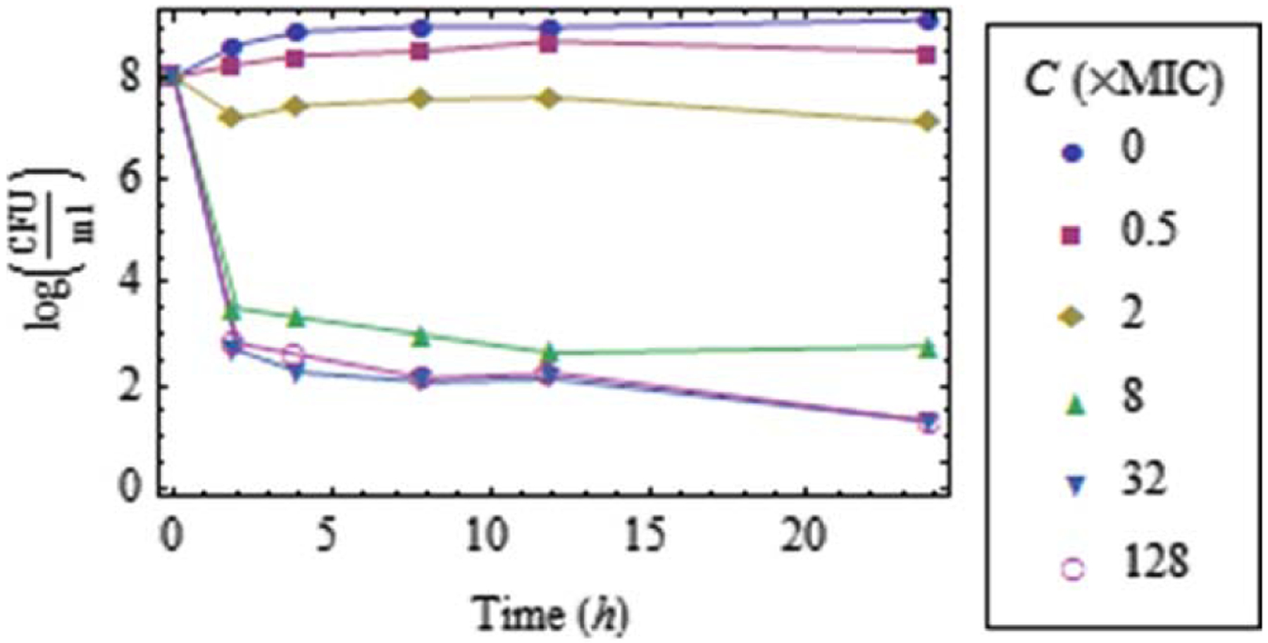
Antibiotic concentration is measured in multiples of the MIC. Details on data collection are provided in Appendix A.

Starting with Eq. 1 for $N\left(t\right)\ll N_{\text{max}}$, Nikolaou and Tam¹⁸ developed explicit expressions for $N\left(t\right)$ and for the distribution of $r\left(C\right)$ over the population as a function of time. The distribution of $r\left(C\right)$ is important for the following reasons:

• The smallest value of $r\left(C\right)$ must be larger than $K_{\text{g}}$ for complete eventual eradication of the entire bacterial population, including its most resistant subpopulation.

• Knowledge of $r\left(C\right)$ as a function of $C$ for the most resistant subpopulation is essential for determining whether a dosing regimen is effective under realistic pharmacokinetic conditions, when repeated cycles of antibiotic injection and exponential decline of $C$ over time during each cycle are encountered. It turns out²² that when the antibiotic is injected every $T$ time units, then the quantity $D\stackrel{\wedge}{=}\frac{1}{T}{\int }_0^T r\left(C\right(t\left)\right)dt$ for the most resistant subpopulation must be larger than $K_{\text{g}}$ for complete eradication of all bacteria.

• An explicit formula for $N\left(t\right)$ would be useful for convenient estimation of the model parameters.

Now, as Figure 1 indicates, experimental data may well be available for a population not far from its saturation point, in which case the population dynamics is nonlinear. For similar reasons as in the linear case, it would be desirable to have an explicit formula for $N\left(t\right)$ and for the distribution of $r\left(C\right)$ over the population as a function of time. Quite remarkably, it turns out that corresponding explicit formulas can be developed for the nonlinear case as well. This is discussed in the next section.

Results

General case

Consider a heterogeneous bacterial population for which the bacterial kill rate induced by an antibiotic at time-invariant concentration $C$ varies among bacteria, with more resistant (less susceptible) bacteria corresponding to lower values of the kill rate constant $r\left(C\right)$. This setting is plausible from a physiological viewpoint, given that variability is expected within any given bacterial species, whether such variability is mild or pronounced. Therefore, the entire bacterial population can be split into a number of subpopulations indexed by $k$, each subpopulation having size $N_k\left(t\right)$, with

$$\sum _k N_k\left(t\right)=N\left(t\right)$$ (3)

Each subpopulation of size $N_k\left(t\right)$ satisfies the counterpart of Eq. 1, namely

$$\frac{d{N}_k}{dt}=\left(K_g\left[1-\frac{N\left(t\right)}{N_{\text{max}}}\right]-r_k\left(C\right)\right)N_k\left(t\right),k=1,2,3,\dots$$ (4)

Note that the term $1-N\left(t\right)/N_{\text{max}}$ is common for all subpopulations, because it refers to competition among bacteria for common resources. Note also that it is important to

In contrast to Eq. 1, of Bernoulli type with the standard closed-form solution

$$N\left(t\right)=N_0\frac{\frac{r\left(C\right)}{K_g}-1}{-\frac{N_0}{N_{\text{max}}}+e^{\left(r\left(C\right)-K_g\right)t}\left(\frac{r\left(C\right)}{K_g}-1+\frac{N_0}{N_{\text{max}}}\right)}$$ (5)

the set of equations in Eq. 4 does not admit a standard solution for $N\left(t\right)$. Furthermore, measuring each subpopulation size $N_k\left(t\right)$ is practically infeasible; rather, only measurements of $N\left(t\right)$ can reasonably be obtained. Therefore, a formula is needed for $N\left(t\right)$ as a function of time for model parameter estimation. In addition, it is of paramount importance to estimate the kill rate $r_k\left(C\right)$ of the most resistant subpopulation, to ensure that an antibiotic concentration $C$ is identified that guarantees eradication of the entire population, including its most resistant subpopulation under in vitro or in vivo pharmacokinetic conditions. It should also be noted that the exact distribution of $r_k\left(C\right)$ over the population is of secondary importance.

Explicit formulas for $N\left(t\right)$ and estimate of $r_k\left(C\right)$ for the most resistant subpopulation are provided next. Note that index $k$ eventually drops out from all results.

Theorem 1. Aggregate dynamics of heterogeneous bacterial population with logistic growth

Assume that a heterogeneous population of $N_0$ bacteria is exposed to an antibiotic at time-invariant concentration $C$. The population has a number of subpopulations, each of which satisfies Eq. 4. Then the aggregate growth or decline of the entire bacterial population is characterized by the following equations

$$\frac{dN}{dt}=\left(K_g\left[1-\frac{N\left(t\right)}{N_{\text{max}}}\right]-\mu \left(t\right)\right)N\left(t\right)$$ (6)

$$\frac{d\mu }{dt}=-\sigma (t{)}^2$$ (7)

$$\frac{d{\sigma }^2}{dt}=-{\kappa }_3\left(t\right)$$ (8)

$$\frac{d{\kappa }_n}{dt}=-{\kappa }_{n+1}\left(t\right),n\ge 3$$ (9)

where

$$\mu \left(t\right)\stackrel{\wedge }{=}\sum _k r_k\left(C\right)\frac{N_k\left(t\right)}{N\left(t\right)}$$ (10)

and

$${\sigma }^2\left(t\right)\stackrel{\wedge }{=}\sum _k {\left[r_k\left(C\right)-\mu \left(t\right)\right]}^2\frac{N_k\left(t\right)}{N\left(t\right)}$$ (11)

are the average and variance, respectively, of the kill rate constant over the entire population at time t; and ${\kappa }_n\left(t\right)$ are the cumulants.^{23, p. 928} of the kill rate constant distribution function

$$f\left(r_k\left(C\right),t\right)\stackrel{\wedge }{=}\frac{N_k\left(t\right)}{N\left(t\right)}$$ (12)

at time $t$, defined through the moment- and cumulant-generating functions, $M(s,t)$ and $\Psi (s,t)$, respectively, as follows

$$M(s,t)\stackrel{\wedge }{=}\sum _k e^{s{r}_k\left(C\right)}f\left(r_k\left(C\right),t\right)$$ (13)

$$\Psi (s,t)\stackrel{\wedge }{=}\text{ln} \left[M\right(s,t\left)\right]=\sum _{n=1}^{\infty } \frac{1}{n!}{\kappa }_n\left(t\right)s^n$$ (14)

$${\left.{\kappa }_n\left(t\right)\stackrel{\wedge }{=}\frac{{\partial }^n\Psi (s,t)}{\partial s^n}\right|}_{s=0},n=1,2,\dots$$ (15)

with ${\kappa }_1\left(t\right)=\mu \left(t\right)$ and ${\kappa }_2\left(t\right)=\sigma (t{)}^2$

Proof. See Appendix B.

Remark 1. Comparison of linear and logistic growth dynamics

Interestingly enough, the equations resulting from Theorem 1, proved for logistic-growth dynamics, are remarkably similar to these in Theorem 1 of Nikolaou and Tam.¹⁸ In fact, Eqs. 7–9 turn out to be similar, whereas Eq. 6 is of the same nature, that is, it is the logistic-growth dynamics counterpart of the linear-growth dynamics equation

$$\frac{dN}{dt}=\left(K_g-\mu \left(t\right)\right)N\left(t\right)$$ (16)

Consequently, the following remarks can be made, which are the counterparts of the linear-growth dynamics case.

• The first four cumulants ${\kappa }_n\left(t\right), n=1,\dots ,4$, are directly related to the average, $\mu$, variance, ${\sigma }^2$, skewness, $\frac{{\mu }_3}{{\sigma }^3}$, and kurtosis excess, $\frac{{\mu }_4}{{\sigma }^4}-3$, of the kill rate constant distribution, namely

  $${\kappa }_1=\mu ,{\kappa }_2={\sigma }^2,{\kappa }_3={\mu }_3,\text{ and }{\kappa }_4={\mu }_4-3{\sigma }^4$$ (17)

  where ${\mu }_{\ell }\left(t\right)$ are the central moments defined as

  $${\mu }_{\mathcal{l}}\left(t\right)=\sum _k {\left(r_k-\mu \left(t\right)\right)}^{\mathcal{l}}f\left(r_k\left(C\right),t\right),\mathcal{l}\ge 0$$ (18)

  for the kill rate constant distribution function $f$.

• Because $-\sigma (t{)}^2\le 0,$ Eq. 7 implies that the average kill rate constant $\mu \left(t\right)$ (a measure of susceptibility or inverse measure of resistance) of a heterogeneous bacterial population will decrease monotonically with time. Furthermore, because $\mu \left(t\right)\ge 0,\mu \left(t\right)$ will converge to a non-negative value. This is because more susceptible bacteria will be preferentially eradicated by the antibiotic over more resistant bacteria, until only the most resistant bacteria, if any, remain in the population.

Theorem 1 can be used to derive closed-form expressions for the time-dependence of the bacterial population size as well as of the average and variance of the kill rate constant distribution, as indicated next.

Theorem 2. Closed-form expressions for time-dependence of population characteristics

Under the assumptions of Theorem 1, the total bacterial population, kill rate constant average, and kill rate constant variance depend explicitly on the moment- and cumulant-generating functions of the initial distribution of the kill rate constant $r\left(C\right)$ as

$$\text{ln} \left[\frac{N\left(t\right)}{N_0}\right]=K_{g}t+\Psi (-t,0)-\text{ln} \left[1+K_g\frac{N_0}{N_{\text{max}}}{\int }_0^t e^{K_g\tau }M(-\tau ,0)d\tau \right]$$ (19)

$$\mu \left(t\right)={\left.\frac{\partial \Psi (s,0)}{\partial s}\right|}_{s=-t}=\mu \left(0\right)-{\sigma }^2\left(0\right)t+\frac{1}{2!}{\kappa }_3\left(0\right)t^2-\frac{1}{3!}{\kappa }_4\left(0\right)t^3+\dots$$ (20)

$$\sigma (t{)}^2={\left.\frac{{\partial }^2\Psi (s,0)}{\partial s^2}\right|}_{s=-t}=\sigma (0{)}^2-{\kappa }_3\left(0\right)t+\frac{1}{2!}{\kappa }_4\left(0\right)t^2-\frac{1}{3!}{\kappa }_5\left(0\right)t^3+\dots$$ (21)

respectively. Moreover, the higher-order cumulants satisfy

$$\begin{gathered} {\kappa }_n\left(t\right)={\left.\frac{{\partial }^n\Psi (s,0)}{\partial s^n}\right|}_{s=-t}={\kappa }_n\left(0\right)-{\kappa }_{n+1}\left(0\right)t+\frac{1}{2!}{\kappa }_{n+2}\left(0\right)t^2 \\ -\frac{1}{3!}{\kappa }_{n+3}\left(0\right)t^3+\dots ,n\ge 3 \end{gathered}$$ (22)

Proof. See Appendix C.

Remark 2. Implications of Theorem 2

• For a population size far from its saturation point, $N_{\text{max}}$, corresponding to approximately linear-growth kinetics, Eq. 19 generalizes the result obtained by Nikolaou and Tam¹⁸ as

  $$\text{ln} \left[\frac{N\left(t\right)}{N_0}\right]=K_{g}t+\Psi (-t,0)$$ (23)

• The terms $\Psi (-t,0)$ and $M(-\tau ,0)$ of Eq. 19, defined in Eqs. 13 and 14, respectively, refer to the cumulant-generating function and to the moment-generating function of the initial bacterial population (they depend on the initial values of the cumulants $\left.{\kappa }_n\left(0\right)\right)$.

• While the initial values ${\kappa }_n\left(0\right)$ of the cumulants may be practically impossible to estimate from experimental data alone, it is demonstrated in the following section that approximations of the initial distribution of the kill rate constant, $r\left(C\right)$, over the bacterial population results in convenient expressions that explicitly contain only a few parameters, which can be estimated from standard experimental data, namely from the size of the bacterial population at a few distinct points in time, measured during time-kill experiments.

Explicit formulas for specific distributions of the kill rate constant

It is interesting to examine the following two special cases of the above results, namely when the initial $r\left(C\right)$ approximately follows the normal or Poisson distribution, because closed-form expressions can be derived.

Normally Distributed Initial Kill Rate Constant.

Strictly speaking, it is impossible to have a distribution of the initial kill rate constant $r\left(C\right)$ that is exactly normal, because that would entail negative values for $r\left(C\right)$. Nevertheless, it is interesting to consider an approximately normally distributed $r\left(C\right)$, because, excluding the first two cumulants (average and variance), all higher-order cumulants of the normal distribution are identically²³

$${\kappa }_n\left(0\right)=0,n\ge 3$$ (24)

In that case, the following explicit formulas can be developed with applicability over limited time $t$.

Theorem 3. Explicit formulas for normally distributed initial kill rate constant

For initially normally distributed $r\left(C\right)$ with average $\mu$ and variance ${\sigma }^2$, it follows that

$$\begin{gathered} \text{ln} \left[\frac{N\left(t\right)}{N_0}\right]=\left(K_g-\mu \right)t+\frac{1}{2}{\sigma }^2{t}^2 \\ -\text{ln} \left[1+K_g\frac{N_0}{N_{\text{max}}}\sqrt{\frac{\pi }{2{\sigma }^2}}\text{exp} \left(\frac{-{\left(K_g-\mu \right)}^2}{2{\sigma }^2}\right)\right. \\ \left.\times \text{erfi} \left(\frac{K_g-\mu \left(0\right)}{\sqrt{2{\sigma }^2}},\frac{K_g-\mu +{\sigma }^{2}t}{\sqrt{2{\sigma }^2}}\right)\right] \end{gathered}$$ (25)

where $\text{erfi} \left(z\right)\stackrel{\wedge}{=}\text{erf} \left(iz\right)/i,\text{erf} \left(z\right)\stackrel{\wedge}{=}\frac{2}{\sqrt{\pi }}{\int }_0^z e^{-t^2}dt$

$$\mu \left(t\right)=\mu -{\sigma }^{2}t$$ (26)

and

$$\sigma (t{)}^2={\sigma }^2$$ (27)

for a time period not exceeding

$$t_{\text{max}}=\frac{\mu }{{\sigma }^2}$$ (28)

In addition, for the same time period,

$${\kappa }_n\left(t\right)=0,n\ge 3$$ (29)

that is, the distribution of $r\left(C\right)$ will remain normal for the same time period.

Proof. See Appendix D.

The above normality assumption yields simple explicit formulas and provides reasonable predictions for relatively short time periods, as has been demonstrated for linear growth dynamics by Nikolaou and Tam.¹⁸ However, the normal distribution assumption is problematic when predictions over longer periods of time are sought, for example, because $\mu \left(t\right)$ Eq. 26, becomes negative. A better alternative is presented next, using a Poisson distribution.

Poisson-Distributed Initial Kill Rate Constant.

Assuming an underlying Poisson distribution for the kill rate constant $r\left(C\right)$ over the initial bacterial population yields explicit formulas that are valid over arbitrarily long time periods and, because they are explicit, they are convenient for parameter identification from total bacterial population time-kill data alone. Specifically, the initial kill rate distribution function is assumed to be

$$f\left(r_k\left(C\right),0\right)\stackrel{\wedge }{=}P[\underset{X}{\underbrace{\frac{r\left(C\right)-r_{min}}{a}}}=k]=\frac{{\lambda }^k{e}^{-\lambda }}{k!},k=0,1,2,\dots$$ (30)

where the average and variance, $\lambda >0$, of the Poisson-distributed variable $X$ are related to the average, $\mu$, and variance, ${\sigma }^2$, of the kill rate constant, $r\left(C\right)\stackrel{\wedge }{=}aX+r_{\text{min}}$, as

$$\mu =a\lambda +r_{min}\ge 0$$ (31)

$${\sigma }^2=a^2\lambda =a\left(\mu -r_{min}\right)\ge 0$$ (32)

The parameter $\lambda >0$ roughly determines the shape of the discrete unimodal distribution $f$, as can be visualized in Figure 2.

Figure 2. Family of the discrete distributions $f\left(r\right)\widehat{=}P\left[r=r_{\text{min}}+ak\right]=\frac{{\lambda }^k{e}^{-\lambda }}{k!},k\ge 0$, for the kill rate constant $r\left(C\right)$ parametrized in terms of $\lambda$ and $r_{\text{min}}$.

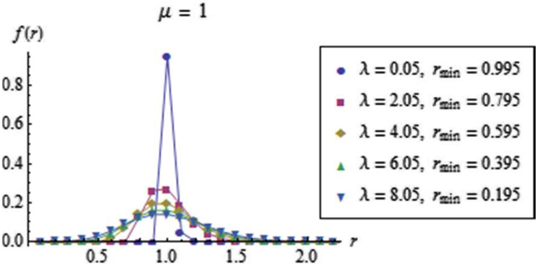
All distributions correspond to the same average $\mu =1$ and $a=1$. Note that $f\left(r\right)=0$ for $r<0$.

Given $\lambda >0$, the parameters ${\sigma }^2$, Eq. 32 and $\mu$, Eq. 31, determine the spread and location of $f$, respectively. Equivalently, the parameters $r_{\text{min}}\ge 0$ and $a>0$ in Eq. 30 are the corresponding parameters for translation and dilation of $r\left(C\right)$, respectively.

Within the above framework, the following explicit formulas can be developed.

Theorem 4. Explicit formulas for Poisson-distributed initial kill rate constant

Given Eq. 30, Eqs. 19, and 21 yield

$$\begin{gathered} \text{ln}\left[\frac{N\left(t\right)}{N_0}\right]=\left(K_{\text{g}}-r_{\text{min}}\right)t+\lambda \left(e^{-at}-1\right) \\ -\text{ln}\left[1+K_{\text{g}}\frac{N_0}{N_{\text{max}}}\underset{0}{\overset{t}{\int }}\text{exp}\left[\left(K_{\text{g}}-r_{\text{min}}\right)\tau +\lambda \left(e^{-a\tau }-1\right)\right]d\tau \right] \\ =\left(K_{\text{g}}-r_{\text{min}}\right)t+\lambda \left(e^{-at}-1\right) \\ -\text{ln}\left[1+K_{\text{g}}\frac{N_0}{N_{\text{max}}}\frac{e^{-\lambda }}{a}{\lambda }^{\frac{K_{\text{g}}-r_{\text{min}}}{a}}{\int }_{\lambda e^{-at}}^{\lambda }{z}^{\frac{r_{\text{min}}-K_{\text{g}}}{a}-1}{e}^{z}dz\right] \end{gathered}$$ (33)

$$\begin{array}{rr}\mu \left(t\right)& =r_{min}+\left(\mu -r_{min}\right)\text{exp} \left[-\frac{\mu -r_{min}}{\lambda }t\right]\\ & =r_{min}+\lambda a{e}^{-at}\end{array}$$ (34)

and

$$\begin{array}{rr}\sigma (t{)}^2& =\frac{{\left(\mu -r_{min}\right)}^2}{\lambda }\text{exp} \left[-\frac{\mu -r_{min}}{\lambda }t\right]\\ & =\lambda a^2{e}^{-at}\end{array}$$ (35)

respectively, where the parameters $r_{\text{min}},a,\mu$, and $\lambda =\frac{\mu -r_{\text{min}}}{a}$ depend on $C$. Note the connections between the integral in Eq. 33 and the incomplete gamma function, defined as

$$\Gamma \left(c,z_0,z_1\right)\stackrel{\wedge}{=}{\int }_{z_0}^{z_1}{z}^{c-1}{e}^{-z}dz$$ (36)

Proof. See Appendix E.

Remark 3. Implications of Theorem 4

• The entire bacterial population will be eradicated if and only if $r_{\text{min}}>K_{\text{g}}$.

• The entire population will eventually be dominated by the most resistant subpopulation, as Eq. 34 implies that ${\text{lim}}_{t\to \infty } \mu \left(t\right)=r_{\text{min}}$.

• The logarithmic part on the right-hand side of Eq. 33 is negligible when the population size $N\left(t\right)$ is far from $N_{\text{max}}$, but becomes significant when $N_{\text{max}}$ is close to $N_{\text{max}}$ (Figure 1).

• Following the convention that a declining bacterial population will be completely eradicated if there exists a time $t>0$ such that $N\left(t\right)=1$, Eq. 33 implies that such time will satisfy the equation

  $$\text{ln} N_0+\left(K_g-r_{min}\right)t+\lambda \left(e^{-at}-1\right)=0$$ (37)

  whose solution is

  $$\frac{\lambda -\text{ln} N_0}{K_g-r_{min}}-\frac{1}{a}\text{ ProductLog }\left(\frac{a\lambda \text{exp} \left[\frac{a\left(\lambda -\text{ln} N_0\right)}{K_g-r_{min}}\right]}{K_g-r_{min}}\right)$$ (38)

  where the function $\text{Product}\text{log} \left(z\right)$ is defined²⁴ as the principal solution, $w$, of the equation $z=w{e}^w$.

• Estimating the dependence of $r_{\text{min}}$ as a function of the antibiotic concentration $C$ (e.g., Eq. 2) is crucial for determining whether a bacterial population will be eventually eradicated or grow, even if there is an initial decline due to elimination of the more susceptible subpopulations.

Figure 3.

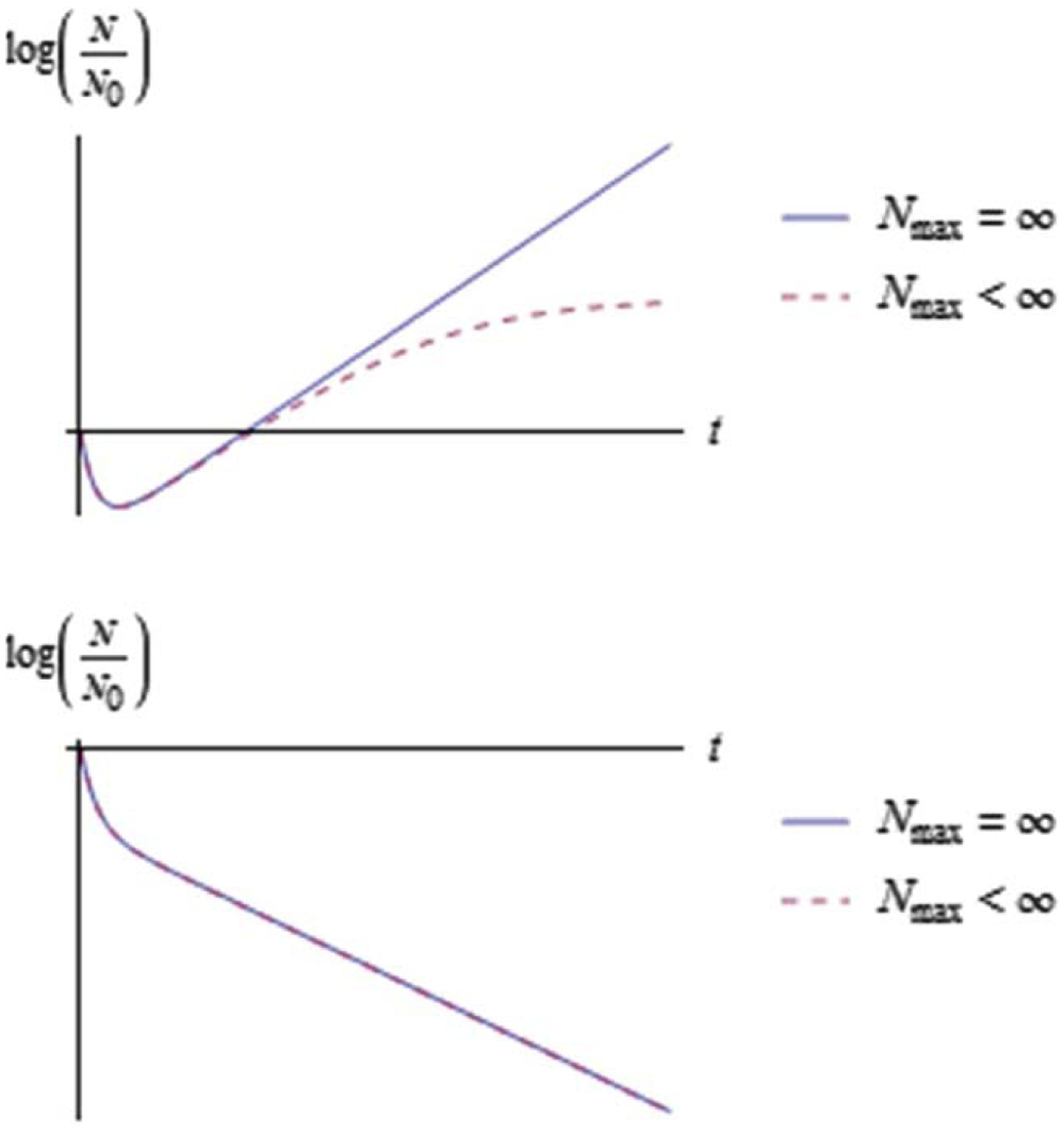
Typical shape of $log \left(\frac{N}{N_0}\right)$ for a heterogeneous bacterial population with $r_{min}<K_g$ (top) and $r_{min}>K_g$ (bottom) when a saturation bound is absent $\left(N_{\text{max}}=\infty \right)$ or present $\left(N_{\text{max}}<\infty \right)$.

Case Study

The mathematical framework developed in the previous Theorem 4 was applied to time-kill data collected for populations of Escherichia coli exposed to the antibiotic moxifloxacin, referred to in Figure 1. Details of the experiments performed are provided in Appendix A.

The parameters $K_{\text{g}}$ and $N_{\text{max}}$ were estimated from the population growth data, corresponding to antibiotic concentration $C=0$, as shown in Figure 2.

Figure 4.

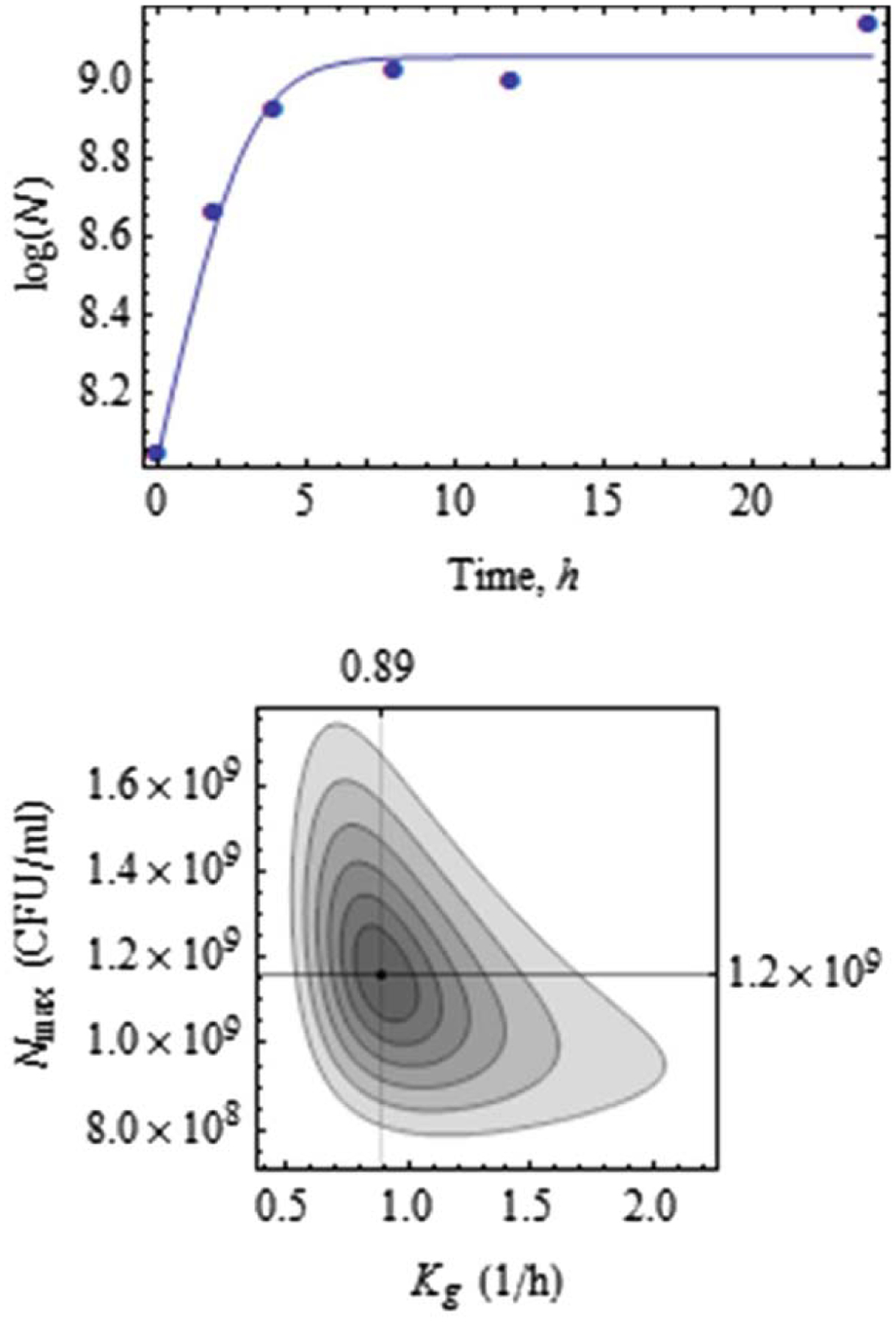
Data fit for $C=0⟺r\left(C\right)=0$ (top) and estimates of $K_g$ and $N_{\text{max}}$ along with confidence regions for confidence levels $1-2^{-k},k=1,\dots ,6$ (bottom).

Using the above estimates of the parameters $K_{\text{g}}$ and $N_{\text{max}}$, time-kill data for antibiotic concentrations $C=0.5\times \text{MIC}$ through $C=128\times \text{MIC}$ were fit by Eq. 33, as shown in Figure 3. The corresponding estimates of the parameters $r_{\text{min}},\lambda$, and $a$ that appear in the model of Eq. 33 are shown in Table 1, for each value of $C$.

Figure 5.

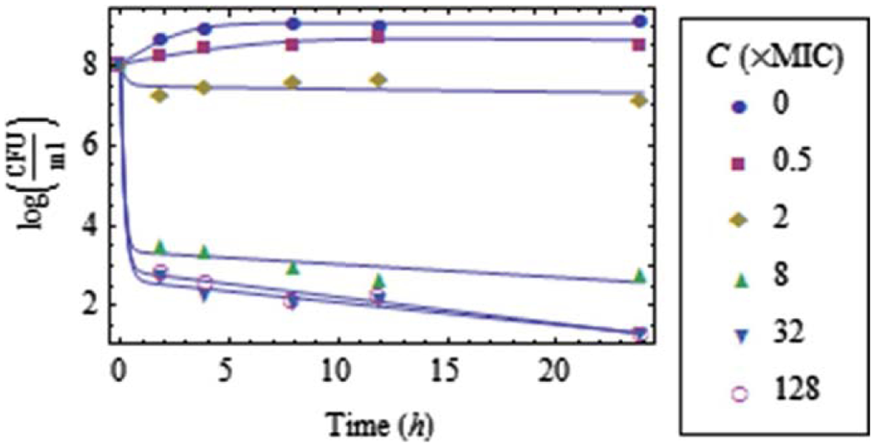
Data fit for $C=0.5\times MIC$ through $C=128\times MIC$ (along with $=0$) using Eq. 33.

Table 1.

Estimates of the Parameters $r_{min},\lambda ,a, for C=0.5\times$ MIC Through $C=128\times MIC (\pm s$ denotes standard error)

$C\left(\times \text{MIC}\right)$	$r_{\text{min}}\pm s\left(1/\text{h}\right)$	$\lambda \left(1/\text{h}\right)$	$a\left(1/\text{h}\right)$
0.5	0.58 ± 0.21	0.38	0.11
2	0.89 ± 0.04	1.3	4.1
8	0.97 ± 0.04	11	6.4
32	1.02 ± 0.03	12	4.9
128	1.04 ± 0.02	12	5.4

The estimates of $r_{\text{min}}$ for $C=0.5\times \text{MIC}$ through $C=128\times \text{MIC}$ can be fitted by Eq. 2 as shown in Figure 4, with corresponding parameter estimates shown in Table 2.

Figure 4.

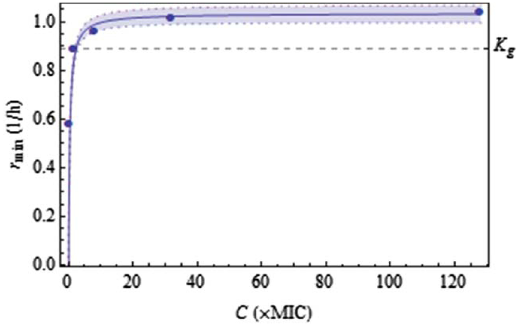
Fit (95% confidence zone) of the kill-rate constant $r_{min}$ as a function of antibiotic concentration C.

Table 2.

Estimates of the Parameters $K_k,C_{50},H$ for the Most Resistant Bacterial Subpopulation

Parameter	Estimate ± Standard Error
$K_k\left(1/\text{h}\right)$	1.03 ± 0.02
$C_{50}\left(\times \text{MIC}\right)$	0.39 ± 0.04
$H$	1.06 ± 0. 15

An important outcome of the above results is that an estimate of the antibiotic concentration $C$ can be easily calculated that ensures eradication of the entire bacterial population, including its most resistant subpopulation. Indeed, eradication is guaranteed if $r_{\text{min}}\left(C\right)=K_{\text{g}}$, which, by Eq. 2, implies

$$C=C_{50}{\left(\frac{K_k-K_g}{K_g}\right)}^{-1/H}=2.2(\times MIC)$$ (39)

as can be visualized in Figure 4. Thus, for this bacterial population, the antibiotic concentration that would ensure complete eradication is more than double the conventional minimum inhibitory concentration (MIC), because of the subpopulations comprising resistant strains.

Discussion

A mathematical modeling framework was developed to describe the effect of antibiotics on heterogeneous bacterial populations (entailing subpopulations of nonuniform susceptibility or resistance to antibiotics). The essence of the framework is captured by Theorem 2, which generalizes and expands prior work developed for antibiotic/bacteria systems following linear dynamics¹⁸ to the case of logistic dynamics. From a practical viewpoint, Theorem 4 offers convenient expressions that can be easily used for parameter estimation based on measurements of an entire bacterial population in time-kill experiments.

Because of its generality, Theorem 2 makes it possible to study the outcomes of various cases, including bimodal distributions.

Appendix A: Details on Experiments Performed for Time-Kill Data Collection

Time-kill studies were performed with a wild-type Escherichia coli strain (MG 1655) with an inoculum of approximately 1 × 10⁸ CFU/mL at baseline. Apart from the placebo control $C=0$, five concentrations of moxifloxacin in Mueller-Hinton broth were used with fourfold increase between subsequent concentrations. All concentrations were normalized to fraction/multiples of the MIC, equal to $0.0625\frac{\mu \text{g}}{\text{mL}}$, from 0.5 × MIC to 128 × MIC. The experiments were performed in a shaker water bath set at 35°C. Serial samples (0.5 mL) were obtained in duplicate over 24 h at baseline, 2, 4, 8, 12 and 24 h; viable bacterial burden was determined by quantitative culture. Before being cultured quantitatively, the bacterial samples were centrifuged (10,000 × G for 15 min at 4°C) and reconstituted with sterile normal saline to minimize the drug carryover effect. Total bacterial populations were quantified by spiral plating 10× serial dilutions of the samples $\left(50\mu \text{L}\right)$ onto Mueller-Hinton agar plates. The media plates were incubated at 35°C for up to 24 h in a humidified incubator, then bacterial density from each sample was enumerated visually.

Appendix B: Proof of Theorem 1

Summation of Eq. 4 over all $k$ yields

$$\begin{gathered} \frac{dN}{dt}=\sum _k\left(K_{\text{g}}\left[1-\frac{N\left(t\right)}{N_{\text{max}}}\right]-r_k\left(C\right)\right)N_k\left(t\right) \\ =\left(K_{\text{g}}\left[1-\frac{N\left(t\right)}{N_{\text{max}}}\right]-\mu \left(t\right)\right)N\left(t\right) \end{gathered}$$ (B1)

which is Eq. 6.

Taking derivatives of Eq. 12 with respect to time and combining it with Eqs. 4 and 6 yields

$$\begin{gathered} \frac{d}{dt}f\left(r_k\left(C\right),t\right)=\frac{d{N}_k}{dt}\frac{1}{N\left(t\right)}-\frac{N_k\left(t\right)}{N{(t)}^2}\frac{dN}{dt} \\ =\left(K_{\text{g}}\left[1-\frac{N\left(t\right)}{N_{\text{max}}}\right]-r_k\left(C\right)\right)N_k\left(t\right)\frac{1}{N\left(t\right)} \\ -\frac{N_k\left(t\right)}{N{(t)}^2}\left(K_{\text{g}}\left[1-\frac{N\left(t\right)}{N_{\text{max}}}\right]-\mu \left(t\right)\right)N\left(t\right) \\ =\left(\mu \left(t\right)-r_k\left(C\right)\right)f\left(r_k\left(C\right),t\right) \end{gathered}$$ (B2)

Taking derivatives of the moment-generating function, Eq. 13, with respect to time, and combining the resulting equation with Eq. B2 yields

$$\begin{gathered} \frac{\partial M\left(s,t\right)}{\partial t}=\sum _k{e}^{s{r}_k\left(C\right)}\frac{df\left(r_k\left(C\right),t\right)}{dt}=\sum _k{e}^{s{r}_k\left(C\right)}\left(\mu \left(t\right)-r_k\left(C\right)\right)f\left(r_k\left(C\right),t\right) \\ =\mu \left(t\right)M\left(s,t\right)-\sum _k{e}^{s{r}_k\left(C\right)}{r}_k\left(C\right)f\left(r_k\left(C\right),t\right) \end{gathered}$$ (B3)

Taking derivatives of the cumulant-generating function, Eq. 14, with respect to time, and combining the resulting equation with Eq. B2 yields

$$\begin{gathered} \frac{\partial \Psi \left(s,t\right)}{\partial t}=\frac{1}{M\left(s,t\right)}\frac{\partial M\left(s,t\right)}{\partial t} \\ =\frac{1}{M\left(s,t\right)}\left[\mu \left(t\right)M\left(s,t\right)-\sum _k{e}^{s{r}_k\left(C\right)}{r}_k\left(C\right)f\left(r_k\left(C\right),t\right)\right] \\ =\mu \left(t\right)-\frac{1}{M\left(s,t\right)}\frac{\partial M\left(s,t\right)}{\partial s} \\ =\mu \left(t\right)-\frac{\partial \text{ln}\left[M\left(s,t\right)\right]}{\partial s} \\ =\mu \left(t\right)-\frac{\partial \Psi \left(s,t\right)}{\partial s} \end{gathered}$$ (B4)

Expanding $\Psi (s,t)$ around $s=0$ using Taylor series as

$$\begin{array}{l}\Psi \left(s,t\right)\underset{0}{\underbrace{\Psi \left(0,t\right)}}+\underset{{\kappa }_1\left(t\right)}{\underbrace{\Psi /\left(0,t\right)s}}+\frac{1}{2!}\underset{{\kappa }_2\left(t\right)}{\underbrace{\Psi //\left(0,t\right)s^2}}+\frac{1}{3!}\underset{{\kappa }_3\left(t\right)}{\underbrace{\Psi ///\left(0,t\right)s^3}}+\dots \\ ={\kappa }_1\left(t\right)s+\frac{1}{2!}{\kappa }_2\left(t\right)s^2+\frac{1}{3!}{\kappa }_3\left(t\right)s^3+\dots \end{array}$$ (B5)

and using the definition of cumulants in Eq. 15 yields

$$\frac{\Psi (s,t)}{\partial t}=\frac{d{\kappa }_1}{dt}s+\frac{1}{2!}\frac{d{\kappa }_2}{dt}{s}^2+\frac{1}{3!}\frac{d{\kappa }_3}{dt}{s}^3+\dots$$ (B6)

and

$$\frac{\Psi (s,t)}{\partial s}={\kappa }_1\left(t\right)+{\kappa }_2\left(t\right)s+\frac{1}{2!}{\kappa }_3\left(t\right)s^2+\frac{1}{3!}{\kappa }_4\left(t\right)s^3\dots$$ (B7)

Substituting the expansions of Eqs. B6 and B7 into Eq. B4 implies

$$\begin{gathered} \frac{d{\kappa }_1}{dt}s+\frac{1}{2!}\frac{d{\kappa }_2}{dt}{s}^2+\frac{1}{3!}\frac{d{\kappa }_3}{dt}{s}^3+\dots = \\ \underset{=0}{\underbrace{\mu \left(t\right)-{\kappa }_1\left(t\right)}}-{\kappa }_2\left(t\right)s-\frac{1}{2!}{\kappa }_3\left(t\right)s^2-\frac{1}{3!}{\kappa }_4\left(t\right)s^3-\dots \end{gathered}$$ (B8)

Equating like powers of $s$ in the above equation yields

$$\frac{d{\kappa }_n}{dt}=-{\kappa }_{n+1}\left(t\right),n\ge 1$$ (B9)

which is Eq. 7 for $n=1$, Eq. 8 for $n=2$, and Eq. 9 for $n\ge 3$

Appendix C: Proof of Theorem 2

Eq. B9 implies

$$\underset{d\kappa /dt}{\underbrace{\left[\begin{array}{c}d{\kappa }_1/dt\\ d{\kappa }_2/dt\\ d{\kappa }_3/dt\\ ⋮\end{array}\right]}}=\underset{\mathbf{J}}{\underbrace{\left[\begin{array}{cccc}0& -1& 0& \ddots \\ \ddots & 0& -1& \ddots \\ \ddots & \ddots & 0& \ddots \\ \ddots & \ddots & \ddots & \ddots \end{array}\right]}}\underset{\kappa \left(t\right)}{\underbrace{\left[\begin{array}{c}{\kappa }_1\left(t\right)\\ {\kappa }_2\left(t\right)\\ {\kappa }_3\left(t\right)\\ ⋮\end{array}\right]}}$$ (C1)

The corresponding solution of the above system of Eq. C1, which is in Jordan form, is

$$\kappa \left(t\right)=\text{exp} \left[\mathbf{J}t\right]\mathbf{\kappa }\left(0\right)=\sum _{k=0}^{\infty } \frac{1}{k!}{\mathbf{J}}^k\kappa \left(0\right)t^k$$ (C2)

from which

$${\kappa }_1\left(t\right)={\kappa }_1\left(0\right)-{\kappa }_2\left(0\right)t+\frac{1}{2!}{\kappa }_3\left(0\right)t^2-\frac{1}{3!}{\kappa }_4\left(0\right)t^3+\dots$$ (C3)

Or

$$\mu \left(t\right)=\mu \left(0\right)-{\sigma }^2\left(0\right)t+\frac{1}{2!}{\kappa }_3\left(0\right)t^2-\frac{1}{3!}{\kappa }_4\left(0\right)t^3+\dots ={\left.\frac{\partial \Psi (s,0)}{\partial s}\right|}_{s=-t}$$ (C4)

which is Eq. 20. Similarly,

$${\kappa }_2\left(t\right)={\kappa }_2\left(0\right)-{\kappa }_3\left(0\right)t+\frac{1}{2!}{\kappa }_4\left(0\right)t^2-\frac{1}{3!}{\kappa }_5\left(0\right)t^3+\dots$$ (C5)

or

$$\sigma (t{)}^2=\sigma (0{)}^2-{\kappa }_3\left(0\right)t+\frac{1}{2!}{\kappa }_4\left(0\right)t^2-\frac{1}{3!}{\kappa }_5\left(0\right)t^3+\dots ={\left.\frac{{\partial }^2\Psi (s,0)}{\partial s^2}\right|}_{s=-t}$$ (C6)

which is Eq. 21, and

$$\begin{gathered} {\kappa }_n\left(t\right)={\kappa }_n\left(0\right)-{\kappa }_{n+1}\left(0\right)t+\frac{1}{2!}{\kappa }_{n+2}\left(0\right)t^2-\frac{1}{3!}{\kappa }_{n+3}\left(0\right)t^3 \\ +\dots ={\frac{{\partial }^n\Psi \left(s,0\right)}{\partial s^n}|}_{s=-t},n\ge 3 \end{gathered}$$ (C7)

which is Eq. 22.

Next, integration of the Bernoulli differential equation in Eq. 6 implies

$$\text{ln} \left[\frac{N\left(t\right)}{N_0}\right]=G\left(t\right)-\text{ln} \left[1+K_{\text{g}}\frac{N_0}{N_{\text{max}}}{\int }_0^t \text{exp} \left[G\right(\tau \left)\right]d\tau \right]$$ (C8)

where

$$G\left(t\right)\stackrel{\wedge }{=}{\int }_0^t \left[K_{\text{g}}-\mu \left(\theta \right)\right]d\theta$$ (C9)

which, by Eq. 20, becomes

$$G\left(t\right)=K_{\text{g}}t+\Psi (-t,0)$$ (C10)

Therefore, substituting $G\left(t\right)$ from the above Eq. C10 into Eq. C8 results in

$$\begin{gathered} \text{ln}\left[\frac{N\left(t\right)}{N_0}\right]=K_{\text{g}}t+\Psi \left(-t,0\right) \\ -\text{ln}\left[1+K_{\text{g}}\frac{N_0}{N_{\text{max}}}{\int }_0^t\text{exp}\left[K_{\text{g}}\tau +\Psi \left(-\tau ,0\right)\right]d\tau \right] \\ =K_{\text{g}}t+\Psi \left(-t,0\right)-\text{ln}\left[1+K_{\text{g}}\frac{N_0}{N_{\text{max}}}{\int }_0^t{\text{e}}^{K_{\text{g}}\tau }M\left(-\tau ,0\right)d\tau \right] \end{gathered}$$ (C11)

which is Eq. 19

Appendix D: Proof of Theorem 3

Equations 27 and 26 follow immediately from Eqs. 20 and 21, along with Eq. 24.

Combining Eqs. 19 and B5 with Eq. 24 yields

$$\text{ln} \left[\frac{N\left(t\right)}{N_0}\right]=K_{\text{g}}t+\mu (-t)+\frac{1}{2!}{\sigma }^2(-t{)}^2-\text{ln} \left[1+K_{\text{g}}\frac{N_0}{N_{\text{max}}}{\int }_0^t \text{exp} \left[\mu (-\tau )+\frac{1}{2!}{\sigma }^2(-\tau {)}^2\right]d\tau \right]=\left(K_{\text{g}}-\mu \right)t+\frac{1}{2}{\sigma }^2{t}^2-\text{ln} \left[1+K_{\text{g}}\frac{N_0}{N_{\text{max}}}{\int }_0^t \text{exp} \left[\left(K_{\text{g}}-\mu \right)\tau +\frac{1}{2}{\sigma }^2{\tau }^2\right]d\tau \right]$$ (D1)

which immediately yields Eq. 25.

Equation 29 follows immediately from Eqs. 24 and 22.

Finally, Eq. 28 follows immediately from Eq. 26 and the fact that $\mu \left(t\right)\ge 0$.

Appendix E: Proof of Theorem 4

The proof follows straightforward facts on moment- and cumulant-generating functions for Poisson distributions and is provided for completeness.

Given Eq. 30, Eq. 13 implies

$$\begin{gathered} M(-t,0)\stackrel{\wedge}{=}\sum _{k\ge 0} e^{-t{r}_k\left(C\right)}f\left(r_k\left(C\right),0\right) \\ =\sum _{k\ge 0} e^{-t\left(ak+r_{\text{min}}\right)}\frac{{\lambda }^k{e}^{-\lambda }}{k!} \\ =\text{exp} \left[-r_{\text{min}}t+\lambda \left(e^{-at}-1\right)\right] \\ =\text{exp} \left[-r_{\text{min}}t+\lambda \left(\text{exp} \left[-\frac{\mu -r_{\text{min}}}{\lambda }t\right]-1\right)\right] \end{gathered}$$ (E1)

which, combined with Eq. 14, implies that the cumulant-generating function is

$$\begin{gathered} \Psi \left(-t,0\right)=\text{ln}\left[M\left(-t,0\right)\right] \\ =-r_{\text{min}}t+\lambda \left(\text{exp}\left[-\frac{\mu -r_{\text{min}}}{\lambda }t\right]-1\right) \\ =-r_{\text{min}}t+\lambda \left(e^{-at}-1\right) \end{gathered}$$ (E2)

Substituting Eqs. E1 and E2 into Eq. 19 immediately yields Eq. 33.

To get a closed-form expression in terms of standard functions for the integral in the nonlinear term of Eq. 33, consider the transformation

$$x\stackrel{\wedge}{=}{e}^{-a\tau }$$ (E3)

to get

$$\begin{gathered} {\int }_0^t\text{exp}\left[\left(K_g-r_{\text{min}}\right)\tau +\lambda \left(e^{-a\tau }-1\right)\right]d\tau \\ ={\int }_1^{e^{-at}}\text{exp}\left[\left(\frac{K_g-r_{\text{min}}}{-a}\right)\text{ln}x+\lambda \left(x-1\right)\right]\frac{dx}{-ax} \\ =\frac{e^{-\lambda }}{a}{\int }_{e^{-at}}^1{x}^{\frac{r_{\text{min}}-K_g}{a}-1}{e}^{\lambda x}dx \\ =\frac{e^{-\lambda }}{a}{\lambda }^{\frac{K_g-r_{\text{min}}}{a}}{\int }_{\lambda e^{-at}}^{\lambda }{z}^{\frac{r_{\text{min}}-K_g}{a}-1}{e}^{z}dz \end{gathered}$$ (E4)

leading to

$$\begin{gathered} \text{ln}\left[\frac{N\left(t\right)}{N_0}\right] =K_{\text{g}}t+\Psi \left(-t,0\right) \\ -\text{ln}\left[1+K_{\text{g}}\frac{N_0}{N_{\text{max}}}{\int }_0^t{\text{e}}^{K_{\text{g}}\tau }M\left(-\tau ,0\right)d\tau \right] \\ =\left(K_{\text{g}}-r_{\text{min}}\right)t+\lambda \left(e^{-at}-1\right) \\ -\text{ln}\left[1+K_{\text{g}}\frac{N_0}{N_{\text{max}}}\frac{e^{-\lambda }}{a}{\lambda }^{\frac{K_{\text{g}}-r_{\text{min}}}{a}}{\int }_{\lambda e^{-at}}^{\lambda }{z}^{\frac{r_{\text{min}}-K_{\text{g}}}{a}-1}{e}^{z}dz\right] \end{gathered}$$ (E5)

Note that the integral ${\int }_{\lambda e^{-at}}^{\lambda } z^{\frac{r_{\text{min}}-K_{\text{g}}}{a}-1}{e}^{z}dz$ always converges because it is over the bounded interval $\left(\lambda e^{-at},\lambda \right)$.

Literature Cited

- 1.Rosenblatt-Farrell N The landscape of antibiotic resistance. Environ Health Perspect. 2009;117(6):A244–A250. [DOI] [PMC free article] [PubMed] [Google Scholar]
- 2.Wright GD. Antibiotic resistance in the environment: a link to the clinic? Curr Opin Microbiol. 2010;13(5):589–594. [DOI] [PubMed] [Google Scholar]
- 3.Varaldo PE. Antimicrobial resistance and susceptibility testing: an evergreen topic. J Antimicrob Chemother. 2002;50:1–4. [DOI] [PubMed] [Google Scholar]
- 4.Neu HC. The crisis in antibiotic resistance. Science. 1992;257:1064–1073 [DOI] [PubMed] [Google Scholar]
- 5.Gold HS, Moellering RC. Antimicrobial-drug resistance. Engl Med. 1996;335:1444–1453. [DOI] [PubMed] [Google Scholar]
- 6.Morens DM, Folkers GK, Fauci AS. The challenge of emerging and re-emerging infectious diseases. Nature. 2004;430:242–249. [DOI] [PMC free article] [PubMed] [Google Scholar]
- 7.Levy SB. The challenge of antibiotic resistance. Sci Am. 1998;278: 46–53. [DOI] [PubMed] [Google Scholar]
- 8.Cohen ML. Epidemiology of drug-resistance-implications for a postantimicrobial era. Science. 1992;257(5073):1050–1055. [DOI] [PubMed] [Google Scholar]
- 9.Drlica KA. Strategy for fighting antibiotic resistance. ASM News. 2001;67(1):27–33. [Google Scholar]
- 10.The White House. Executive Order-Combating Antibiotic-Resistant Bacteria. 2014. Available at: http://www.whitehouse.gov/the-press-office/2014/09/18/executive-order-combating-antibioticresistant-bacteria.
- 11.Giraldo J, Vivas NM, Vila E, Badia A. Assessing the (a)symmetry of concentration-effect curves: empirical versus mechanistic models. Pharmacol Therapeut. 2002;95:21–45. [DOI] [PubMed] [Google Scholar]
- 12.Lipsitch M, Levin BR. The population dynamics of antimicrobial chemotherapy. Antimicrob Agents Chemother. 1997;41(2):363–373. [DOI] [PMC free article] [PubMed] [Google Scholar]
- 13.Nicolau DP, Onyeji CO, Zhong M, Tessier PR, Banevicius MA, Nightingale CH. Pharmacodynamic assessment of cefprozil against Streptococcus pneumoniae: implications for breakpoint determinations. Antimicrob Agents Chemother. 2000;44(5):1291–1295. [DOI] [PMC free article] [PubMed] [Google Scholar]
- 14.Andes D, Craig WA. In vivo activities of amoxicillin and amoxicillin-clavulanate against Streptococcus pneumoniae: application to breakpoint determinations. Antimicrob Agents Chemother.1998;42(9):2375–2379. [DOI] [PMC free article] [PubMed] [Google Scholar]
- 15.Dandekar PK, Tessier PR, Williams P, Nightingale CH, Nicolau DP. Pharmacodynamic profile of daptomycin against Enterococcus species and methicillin-resistant Staphylococcus aureus in a murine thigh infection model. J Antimicrob Chemother. 2003;52(3):405–411. [DOI] [PubMed] [Google Scholar]
- 16.Miyazaki S, Okazaki K, Tsuji M, Yamaguchi K. Pharmacodynamics of S-3578, a novel cephem, in murine lung and systemic infection models. Antimicrob Agents Chemother. 2004;48(2):378–383. [DOI] [PMC free article] [PubMed] [Google Scholar]
- 17.Oliver A, Levin BR, Juan C, Baquero F, Blazquez J. Hypermutation and the preexistence of antibiotic-resistant Pseudomonas aeruginosa mutants: implications for susceptibility testing and treatment of chronic infections. Antimicrob Agents Chemother. 2004;48(11): 4226–4233. [DOI] [PMC free article] [PubMed] [Google Scholar]
- 18.Nikolaou M, Tam VH. A new modeling approach to the effect of antimicrobial agents on heterogeneous microbial populations. J Math Biol. 2006;52(2):154–182 [DOI] [PubMed] [Google Scholar]
- 19.Jusko W Pharmacodynamics of chemotherapeutic effects: dose-time-response relationships for phase-nonspecific agents. J Pharm Sci. 1971;60:892–895. [DOI] [PubMed] [Google Scholar]
- 20.Wagner J Kinetics of pharmacologic response I. proposed relationships between response and drug concentration in the intact animal and man. J Theor Biol. 1968;20:173–201. [DOI] [PubMed] [Google Scholar]
- 21.Hill AV. The possible effects of the aggregation of the molecules of haemoglobin on its dissociation curves. J Physiol. 1910;40:iv–vii. [Google Scholar]
- 22.Nikolaou M, Schilling AN, Vo G, Chang K-t, Tam VH. Modeling of microbial population responses to time-periodic concentrations of antimicrobial agents. Ann Biomed Eng. 2007;35(8):1458–1470. [DOI] [PubMed] [Google Scholar]
- 23.Abramowitz M, Stegun IA, editors. Handbook of Mathematical Functions with Formulas, Graphs, and Mathematical Tables, 9th printing. New York: Dover, 1972. [Google Scholar]
- 24.Corless RM, Gonnet GH, Hare DEG, Jeffrey DJ, Knuth DE. On the Lambert W function. Adv Comput Math. 1996;5:329–359. [Google Scholar]