Principles of fluorescence correlation spectroscopy applied to studies of biomolecular liquid–liquid phase separation

Abstract

Fluorescence correlation spectroscopy (FCS) investigates the temporal relationship of fluctuating fluorescence signals reflecting underlying molecular processes occurring in a solution sample or a single live cell. This review article introduces the principles of two basic and most used FCS techniques: fluorescence auto-correlation spectroscopy (FACS) and fluorescence cross-correlation spectroscopy (FCCS). Combined, FACS and FCCS techniques can quantitatively analyze multiple properties of molecule or nanoparticle samples, including molar concentration, diffusion coefficient and hydrodynamic radius, homo- or hetero-interaction, fluorescence brightness, etc. Not surprisingly, FCS techniques have long been used to investigate molecular mechanisms of biomolecular phase separation, first in the lipid bilayer and more recently in cell cytosol and nucleoplasm. The latter applications are especially exciting since a whole new class of membraneless cellular organelles have been discovered, which are proposed to be results of biomolecule liquid-liquid phase separation (LLPS). LLPS research can benefit significantly from the multifunctionality and single-molecule sensitivity of a variety of FCS techniques, particularly for live-cell studies. This review illustrates how FACS and FCCS techniques can be used to investigate multiple aspects of the molecular mechanisms of LLPS, and summarizes FCS applications to LLPS research in vivo and in vitro.

INTRODUCTION TO FLUORESCENCE CORRELATION SPECTROSCOPY

Traditional fluorescence spectroscopy investigates photophysical properties of fluorescence photons, such as excitation and emission spectra, polarization, lifetime, quenching, energy transfer, etc. In contrast, fluorescence correlation spectroscopy (FCS) and image correlation spectroscopy (ICS) analyze relationships (i.e., correlation) of fluorescence signals in temporal and spatial domains, respectively. This review focuses on the FCS techniques. Excellent reviews regarding the ICS techniques can be found elsewhere (Hebert et al. 2005; Kolin and Wiseman 2007; Petersen et al. 1993). Temporal relationships of fluorescence signals are caused by underlying physical (e.g., diffusion) and/or chemical (e.g., binding) molecular processes. Thus, FCS can be used to investigate physical (e.g., diffusional coefficient, hydrodynamic radius) and chemical (e.g., concentration, binding affinity) properties of fluorescent or fluorescently labeled molecules. The theoretical foundation of FCS was established in the early 1970s (Ehrenberg and Rigler 1974; Elson and Magde 1974; Magde et al. 1972, 1974), and its mathematic formulation is similar to that of dynamic light scattering (DLS). DLS utilizes the nonspecific and much weaker signal of scattered photons, thus requiring purified and concentrated sample solutions. Using specific and highly amplified fluorescent photons, FCS has the ultimate sensitivity (i.e., single molecule) and can investigate molecular properties in a heterogeneous environment (e.g., within a single live cell). In fact, FCS is the first single-molecule fluorescence technique (Eigen and Rigler 1994). Widespread applications of FCS methods only began in the early 1990s, after the development and maturation of laser, detector, computer, microscope, fluorescence label, data acquisition and analysis technologies. Today, there have been >12,000 papers in PubMed published using a variety of FCS techniques, covering research fields of biology, medicine, chemistry, physics, nanotechnology, etc. FCS has been proved to be a versatile tool for investigating molecular properties in aqueous solutions or in single live cells. Through auto- or cross-correlation analysis of temporally fluctuating fluorescence signals collected from an ultra-small open volume (~1 femtoliter; fL), FCS can quantify molecular properties such as concentration (pmol/L–nmol/L), size (hydrodynamic radius) and interaction (K_D value) with single-molecule resolution (Elson 2011; Haustein and Schwille 2003; Hess et al. 2002; Wang et al. 2018). Particularly, FCS has long been used to investigate phase separation processes in the lipid bilayer (Chiantia et al. 2009; Eggeling et al. 2009; He and Marguet 2011; Korlach et al. 1999; Mueller et al. 2013). Recently, FCS has been applied to studies of biomolecular liquid–liquid phase separation (LLPS) in vivo or in vitro. This review will first explain, at a basic level, principles of FCS analysis, and then summarize FCS applications to LLPS studies in live cells and in aqueous solutions.

PRINCIPLES OF FLUORESCENCE CORRELATION SPECTROSCOPY

The most updated and comprehensive explanation of the FCS techniques can be found in a recently published book entitled “An Introduction to Fluorescence Correlation Spectroscopy” by IOP Publishing (Bristol, UK) (Wohland et al. 2020). Interested readers are strongly recommended to study this book for an in-depth understanding of a variety of fluorescence correlation methods, their capabilities, applications and pitfalls. Below, we introduce the two basic and most widely used FCS techniques: fluorescence auto-correlation spectroscopy (FACS; often just referred to as FCS) and fluorescence cross-correlation spectroscopy (FCCS). These two techniques analyze quantitatively these fundamental molecular properties: molar concentration, diffusion coefficient and hydrodynamic radius, hetero- and homo-interactions. In addition, the brightness of fluorescently labeled molecules can also be estimated experimentally. These analytical capabilities, utilized separately or in combination, provide powerful means of investigating molecular mechanisms of LLPS, in live cells or in aqueous solutions. We attempt to explain the principles of FCS analysis both in intuitive and quantitative ways.

The most distinguishing feature of FCS techniques is to investigate molecular properties in an equilibrium solution. Typical approaches to investigate chemical reactions using the “perturbation-monitoring” method: e.g., adding reactants A and B together at time zero (i.e., experiment starts), then monitoring the formation of the binding product AB until the reaction reaches equilibrium:

Here, the association rate constant k_f is much larger than the dissociation rate constant k_b, and brackets represent molar concentrations. In contrast, FCS techniques often start with a sample solution already in equilibrium! In this case, one of the reactants is labeled with a fluorescent probe (A^*), and the chemical reaction either causes A^* to diffuse slower (by forming the A^* B product), and/or results in stronger or weaker A^* fluorescence:

Obviously, for a bulk solution in chemical equilibrium, the amount of AB formation equals that of its dissociation. Thus, the total fluorescence of the bulk sample remains constant and yields no information about the underlying reaction kinetics. However, if we can isolate a microscopic part of the bulk sample, within which chemical reaction occurs with single or a few molecules, then the association and dissociation rates are stochastically determined by individual thermodynamic energies associated with these molecules, causing instant unbalancing of the chemical reaction:

Such instant perturbations are reflected by fluorescence fluctuations observed from the microscopic part of the sample. Auto- or cross-correlation analysis of the fluctuating fluorescence signals can then uncover the underlying rate constants associated with the chemical reaction.

For FCS techniques, this microscopic part of the bulk solution is isolated using a focused laser beam created by a microscope optical pathway. We call this microscopic part as “FCS volume element V” (Fig. 1). V is very small, typically less than one femtoliter (1 fL = 10⁻¹⁵ L), within which single or few (<100) non-interacting fluorescent molecules of the same species diffuse freely. V is also an open volume in a sample solution, so fluorescently labeled molecules can diffuse in and out of it. At any moment t, there are N(t) number of fluorescent molecules within V. N(t) is stochastically determined by the few freely diffusing molecules sampled by the FCS volume element V at time t. In fact, N(t) obeys Poisson statistics, thus its time averaged (represented by angle brackets) value <N(t)> equals its variance <δN(t)²>:

Figure 1.

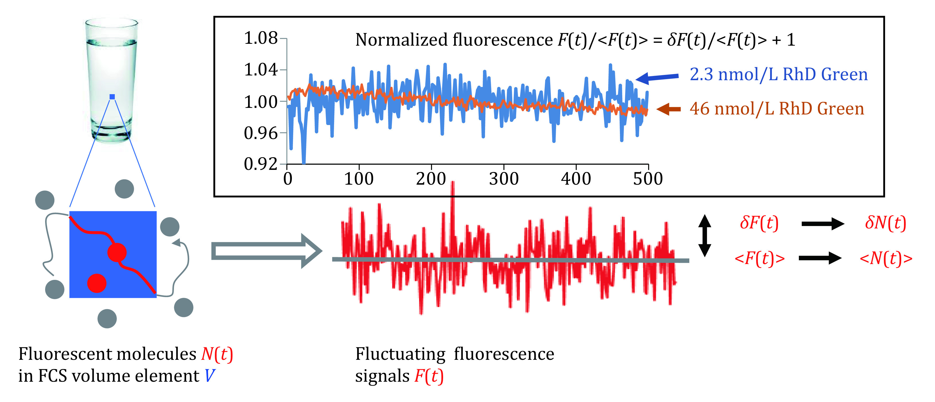
Correlation between fluctuating fluorescence signals and numbers of freely diffusing fluorescent molecules within a microscopic volume (i.e., FCS volume element) of a bulk sample solution. Inset shows normalized fluorescence intensities of two Rhodamine Green samples obtained from such an FCS volume element

1

In Eq. 1, δN(t) = N(t) – <N(t)>, indicating instant deviations of the numbers of fluorescent molecules within V from the time averaged value. For a single fluorescent species of equal molecular brightness, the average number of fluorescent molecules <N(t)> and its instant fluctuations δN(t) are reflected respectively by the average fluorescence intensity <F(t)> and its intensity fluctuations δF(t) (Fig. 1). Thus,

2

In Eq. 2, δF(t) = F(t) – <F(t)>. As mentioned above, auto-correlation analysis of the fluctuating fluorescence signal F(t) can uncover underlying molecular properties. The auto-correlation function is defined as:

3

In Eq. 3, G(τ) is the auto-correlation amplitude and τ is the correlation time. Setting τ = 0 and substituting Eq. 2, Eq. 3 becomes:

4

Equation 4 indicates that the normalized fluorescence fluctuation amplitude <δF(t)²>/<F(t)>² is inversely proportional to the average fluorescence intensity <F(t)>. This inverse relationship can be experimentally verified (inset in Fig. 1): i.e., under the same experimental conditions, the average fluorescence intensity of a 2.3 nmol/L Rhodamine (RhD) Green sample is obviously much weaker than that of a 46 nmol/L RhD Green sample; yet, the normalized fluorescence fluctuation amplitudes of the former are much bigger than those of the latter. Equation 4 can be rewritten using the number of fluorescent molecules N(t) within V and its instant fluctuation δN(t):

5

In Eq. 5, C is the molar concentration of a sample solution and N_A is the Avogadro constant. Combined, Eqs. 4 and 5 indicate that auto-correlation analysis of a fluctuating fluorescence signal F(t) can determine the G(0) value (Eq. 4), from which molar concentration can be calculated (Eq. 5). Of course, we also need to determine the FCS volume element V, which is typically done using a 1–10 nmol/L calibration sample containing a fluorescent dye (e.g., Alexa488, ATTO655) with a known concentration or diffusion coefficient (see below).

Equation 4 seems to suggest that the G(0) value can be directly calculated through inversion of the average fluorescence intensity (i.e., 1/<F(t)>). In reality, the experimentally detected <F(t)> contains not only fluorescence photons originated from samples molecules in V, but also background signals (e.g., solvent scattered light, intrinsic fluorescence), detector noises (e.g., dark current, after pulse), etc. Thus, the correct G(0) value is determined indirectly through quantitative evaluation of the auto-correlation function over a wider range of correlation times (i.e., 0 < τ < ∞), as explained below.

Equation 5 indicates that there shall not be too many fluorescent molecules within the FCS volume element V. For example, if there are more than 1000 molecules in V, G(0) will be less than 0.001, then the normalized fluorescence fluctuation amplitudes will be too small to be instrumentally evaluated (Eq. 4). If V = 1 fL, then 1000 molecules within it are equivalent to a molar concentration of 1.66 μmol/L. Biomolecule concentrations in live cells are typically in the μmol/L range, thus we shall make V as small as possible so that FCS techniques can be applied to live-cell studies. The smallest 3D-volume, from which fluorescence signals are collected, actually defines a fluorescence microscope’s axial and lateral resolutions. Thus, pursuing the smallest signal collection volume is the unified goal of FCS and fluorescence microscopy. The spatial resolution of conventional fluorescence microscopy is principally determined by the numeric aperture (NA) of a microscope objective as well as the wavelength of fluorescence emission. Furthermore, FCS typically investigates molecule diffusion in an aqueous solution. Thus, a water-immersion, high-NA objective with correction collar for compensating glass coverslip thickness (e.g., Olympus 60X 1.2NA water-immersion objective) is usually employed for FCS experiments. FCS analysis has been adapted to most high-resolution fluorescence microscopes, including confocal, multiphoton, TIRF, light-sheet, etc. In addition, FCS is compatible with stimulated emission depletion (STED) super-resolution fluorescence microscopy (Honigmann et al. 2014; Mueller et al. 2013). A much smaller FCS volume element defined by STED microscopy allows fluorescent samples with higher molecular concentrations (Eq. 5). More importantly, a smaller FCS probing volume enables precise investigation of biologically important structures such as “lipid rafts” that are smaller than the spatial resolution of conventional fluorescence microscopy (Honigmann et al. 2014; Mueller et al. 2013). Overall, a combination of fluorescence imaging and correlation analysis enables not only visualization of subcellular structures in a live cell, but also the investigation of molecular mechanisms on the subcellular structures!

Figure 2A shows an FCS device built upon a confocal optical pathway. The laser beam is focused into a sample solution via a high numeric aperture, water-immersion objective. Fluorescent molecules within the focal pathway are excited and resulting fluorescence signals are partially collected by the same objective, reflected by a dichroic mirror, cleaned up by a filter before being detected by a single-photon counting avalanche photodiode (SPAD). The key for confocal microscopy is to place a confocal pinhole of suitable size and position in front of the SPAD. The function of this pinhole is to further restrict a fluorescence signal collection volume (i.e., FCS volume element V) within the focal spot in the sample solution (Fig. 2B, bottom). Within the elliptically shaped volume element, the laser intensity is highest at the center (I₀) and decays approximately in Gaussian modes both in the axial and lateral directions. The boundaries of V are defined at r₀ and z₀, where laser intensities decay to 1/e² of I₀ along with lateral and axial directions respectively. When a single fluorescently labeled molecule diffuses through V, its fluorescence intensity along the diffusing pathway will match laser intensities along the pathway. In an ideal experiment, when a single molecule diffuses straight through the center of the FCS volume element in the lateral direction, it will produce an ideal single-molecule fluorescence (SMF) signal δF(t) that ignores background signals and detector noises. δF(t) has a Gaussian shape and its width reflects the time for this molecule to diffuse through V (Fig. 2B, bottom). Obviously, a big molecule with a smaller diffusion coefficient will produce a wider δF(t), and a small molecule with a narrower δF(t). Thus, SMF signals acquired from the FCS volume element contain information about molecular size! The experimentally acquired fluorescence signal F(t) is a linear combination of a limited number of SMF signals at any moment t (Fig. 2, top). These SMF signals do not have the ideal Gaussian shape, but nevertheless still contain information about molecule size. Auto-correlation analysis of the experimentally collected F(t) will yield quantitative results about a sample molecule’s diffusion coefficient as well as its hydrodynamic radius.

Figure 2.

Fluorescence signals collected from an FCS volume element created through a confocal optical pathway. A Confocal optical pathway. B Bottom: FCS volume element and an ideal single molecule fluorescence signal; top: real fluorescence signals collected from the FCS volume element

Within the framework of the ideal SMF experiment discussed above. The auto-correlation function (Eq. 3) can be visualized as finding the overlapping area between the original SMF signal δF(t) and its replicate signal δF(t + τ), with δF(t + τ) being shifted on the horizontal time axis by a τ unit (Fig. 3A). When τ = 0, δF(t) and δF(t + τ) completely overlap, thus producing the biggest auto-correlation amplitude G(0) (Fig. 3B). When τ = τ_D, approximately half of the δF(t) and δF(t + τ) areas overlap, producing a G(τ_D) amplitude that is roughly half of the G(0) amplitude. The characteristic diffusion correlation time τ_D indicates how fast the auto-correlation function G(τ) decays. In our ideal SMF experiment, δF(t) width is ~2τ_D; thus, τ_D is related to molecular size! When τ → ∞, δF(t) and δF(t + τ) completely separate on the time axis, thus G(∞) → 0. Overall, τ increase results in G(τ) decrease, producing an auto-correlation decay curve shown in Fig. 3B. From the G(0) value of the decay curve, we can derive the molar concentration of a sample solution (Eq. 5), and from the τ_D value, we can calculate the diffusion coefficient and hydrodynamic radius of the sample molecule (see below). Importantly, our pictorial explanation of the auto-correlation analysis can be extended to the experimentally acquired fluorescence signal F(t) (Fig. 2B, top). Essentially, the auto-correlation function (Eq. 3) is a mathematic funnel: i.e., inputting the fluctuating fluorescence signals F(t), outputting the auto-correlation decay curve; from the latter molar concentration and diffusion coefficient of a fluorescent molecule can be precisely measured.

Figure 3.

Pictorial explanation of fluorescence auto-correlation analysis. A Auto-correlation of an ideal single molecule fluorescence signal. B Corresponding auto-correlation decay curve of the ideal single molecule fluorescence signal

Auto-correlation computation can be accomplished using a hardware correlator (Eid et al. 2000; Gamari et al. 2014) or through software algorithms (Magatti and Ferri 2003; Schaub 2013), producing discrete G(τ) data shown in Fig. 3B. Quantitative interpretation of the G(τ) data requires the mathematic modeling of three-dimensional (3D) molecular diffusion sampled by the FCS volume element V (Fig. 2B, bottom). Assuming a uniform solution containing one species of non-interacting fluorescent molecules, the analytical solution to the auto-correlation function, in terms of 3D-molecular diffusion, is (Elson and Magde 1974; Krichevsky and Bonnet 2002):

6

In Eq. 6, N = <N(t)>, and S describes the ellipticity of the FCS volume element V (Fig. 2B, bottom), with S = z₀/r₀ (Fig. 2B, bottom). Using Eq. 6 and setting N, τ_D and S as fitting parameters, raw G(τ) data (black dots in Fig. 3B) can be quantitatively analyzed via a nonlinear least squared fitting algorithm (red line in Fig. 3B), producing experimentally determined values of N, τ_D and S. It shall be noted that FCS experiments are interfered by background signals (i.e., F(t)_BG), such as contaminant fluorescence, scattered light, detector dark current and after pulse. If the background signals are not correlated (i.e., G(τ)_BG is approximately flat and equals to 1), then the shape of G(τ) and hence τ_D value are not affected. However, the experimentally determined G(0) value needs to be scaled (Hess et al. 2002) so that: G(0)_cor = G(0)<F(t)>²/[<F(t)> – <F(t)>_BG]², with <F(t)> and <F(t)>_BG being experimentally measured sample and background time-averaged photon signals respectively. If the background signals (e.g., contaminant fluorescence) correlate, then τ_D value cannot be precisely determined. Nevertheless, if <F(t)>_BG is less than 5% of <F(t)>, it its acceptable to ignore background interference during an FCS experiment (Hess et al. 2002).

Since S is determined theoretically only by the confocal optical pathway (Fig. 2A), particularly the pinhole size and location, S value is often measured using a calibration sample (typically a 1–10 nmol/L dye solution) and then fixed during the subsequent analysis of experimental data. It is advisable to determine the S value for each FCS experiment session. Constant S values indicate stability in the optical pathway and instrument performance. Furthermore, from the experimentally determined τ_D value, we have:

7

In Eq. 7, D is the diffusion coefficient of a sample molecule. τ_D represents the average time for sample molecules to diffuse through the FCS volume element V (Fig. 2B, bottom), thus it is proportional to r₀ but inversely proportional to D. D is related to the hydrodynamic radius of a sample molecule or nanoparticle through the Stoke-Einstein equation:

8

In Eq. 8, K_B is the Boltzmann constant, T is absolute temperature, η is solvent viscosity and R_H is the hydrodynamic radius of a sample molecule or nanoparticle. It shall be noted that both D(T) and η(T) are temperature dependent, thus results obtained from FCS experiments carried out in different buffers and at different temperatures shall be carefully calibrated. For a calibration sample of 10 nmol/L ATTO655 solution, the dye’s diffusion coefficient at 25 °C has been precisely determined (Dertinger et al. 2007) to be (4.26 ± 0.08) × 10⁻⁶ cm²/s. Hence this calibration sample can be used to determine S and r₀ values of the FCS volume element V via Eqs. 6 and 7. Subsequently, FCS volume element V and molar concentration C of another sample can then be calculated:

9

Overall, Eqs. 6–9 summarize the analytical steps for determining a fluorescent molecule’s molar concentration, its diffusion coefficient and hydrodynamic radius. This procedure typically requires a calibration sample containing a dye molecule with a known diffusion coefficient, then the molar concentrations and diffusion coefficients of other molecules can be subsequently measured. A third useful parameter, molecular brightness λ, can also be estimated from an FCS experiment:

10

Molecular brightness is a function of laser power, instrument fluorescence collection efficiency, a fluorescent probe’s absorption extinction coefficient and fluorescence quantum efficiency. However, for FCS experiments carried out under the same conditions, λ value is a useful indicator of the biomolecular homo-oligomerization state. For example, for a protein molecule tagged with a GFP probe, its dimer shall be roughly twice as bright as its monomer.

As mentioned above, FCS techniques can analyze rate constants of a chemical reaction in equilibrium, provided such reaction resulting in changes in fluorescence probe’s brightness. A classic example of such a reaction, photophysical in nature, is the constant cycling of a fluorescence probe in its excited singlet or triplet states (Fig. 4A). Typically, after a fluorescent molecule absorbs the energy of an excitation photon (hν₁; h is the Planck constant, ν is the frequency of the photon), an electron in the outmost orbit of the fluorescent molecule transits from its ground state (S₀) to the first excited electronic state (S₁). The excited electron in the S₁ state (black circle in Fig. 4A) is unstable; typically, after a few nanoseconds (i.e., fluorescence lifetime), this electron decays back to its S₀ state, emitting a fluorescence photon (hν₂) with a less than 100% probability (i.e., fluorescence quantum efficiency). Very rarely, the excited electron in the S₁ state spontaneously flips its spin direction, thus transits to the triplet state (T; i.e., intersystem crossing); now the excited electron has the same spin direction as that of the pairing electron still remaining in the S₀ state (grey circle in Fig. 4A). Quantum mechanisms thus prohibit this excited electron in the triplet state from returning to the ground state. Only after a relatively long time, typically microseconds to seconds (i.e., phosphorescence lifetime), when the electron in the triplet state experienced another spontaneous spin flip, it is allowed to decay back to the S₀ state, with a very small probability of emitting a phosphorescence photon (hν₃). When the fluorophore is cycling between the S₀ S1 states, it constantly emits fluorescence photons and appears to be bright. In contrast, when the molecule is trapped in the triplet state, it only very rarely emits a phosphorescence photon and appears to be dark. Thus, fluorophore cycling between the singlet and triplet states (i.e., triplet dynamics) can be described by a simple photophysical reaction:

Figure 4.

Effect of fluorophore triplet dynamics on the auto-correlation decay curve of a freely diffusing fluorescent molecule. A Energy diagram of single-triplet transition. B Effect of triplet dynamics on a fluorescence auto-correlation decay curve

The rate of such cycling is defined by a relaxation constant τ_T = 1/(k_f + k_b), with k_f and k_b being the forward and backward reaction rate constants respectively. Incorporating the triplet dynamics, the analytical solution to the auto-correlation function for one species of fluorescent molecules diffusing in 3D-space becomes:

11

In Eq. 11, T indicates the fraction of N fluorescent molecules trapped in the triplet state. The three multiplication units on the right side of Eq. 11 can be represented by G(0), G(τ)_T and G(τ)_D respectively, thus:

12

In Eq. 12, the auto-correlation function G(τ) is broken into three parts, G(0), G(τ)_T and G(τ)_D, with the latter two accounting for the triplet dynamics and 3D molecular diffusion respectively. Usually, τ_T is less than ten microseconds while τ_D for a biomolecule is larger than one millisecond. Under this circumstance, the G(τ)_T and G(τ)_D phases of the auto-correlation decay are well separated, and the relationship among G(0), G(τ)_T and G(τ)_D is shown in Fig. 4B. It shall be noted that although Eq. 11 is derived assuming a fluorophore undergoing single (bright) triplet (dark) cycling, it also applies to any chemical reaction causing the fluorophore to become brighter or dimmer. Since FCS experiments require fluorescent labeling and essentially all fluorophores undergo triplet dynamics, Eq. 11 is a universal fitting model for analyzing FCS data of single species molecular diffusing in 3D space. Of course, we can ignore G(τ) data under a certain τ threshold (i.e., τ < 10 μs); in this case, Eq. 6 is sufficient to analyze single species molecular diffusion in 3D space with minimum interference from a fluorophore’s triplet dynamics.

If there are i^th species of fluorescent molecules freely diffusing in a sample solution and these molecules do not interact with each other, then the analytical solution to the auto-correlation function is:

13

In Eq. 13, λ_i is the brightness, N_i is the average number within the FCS volume element, and G_i(τ)_D is the diffusional auto-correlation decay of the i^th fluorescent molecule species, respectively. f_i represents the contribution of the i^th fluorescent species to the overall fluorescence auto-correlation decay curve. Importantly, such contribution is dependent on the square of molecule brightness (λ_i²). Thus, bright molecules contribute disproportionally to the overall auto-correlation decay curve for a sample containing multiple fluorescent species. For a simple biomolecular binding reaction, such as antigen-antibody binding, Eq. 13 becomes:

14

In Eq. 14, Molecule One could be the smaller and fluorescently labeled antigen (Ag*; the antibody is unlabeled), and Molecule Two the antigen–antibody binding product (Ag*Ab); τ₁ and τ₂ are then characteristic diffusion correlation times for Ag* and Ag*Ab respectively. In this case, τ₂ shall be at least ~60% larger than τ₁ for the FCS analysis to distinguish two different diffusional species (i.e., Ag* and Ag*Ab) in the sample solution (Meseth et al. 1999). Diffusion correlation time τ_D scales linearly with molecular hydrodynamic radius R_H (Eqs. 7 and 8), and R_H can be roughly estimated to be the cubic root of molecule weight (MW). Thus, MW of Ag*Ab needs to be at least ~4 folds bigger than that of Ag*. If this condition is satisfied, FCS experiments have been successfully implemented to determine the dissociation constants (K_D) of biomolecular binding reactions (Tetin et al. 2013; Luo et al. 2021).

If the two interacting molecules (e.g., M₁ and M₂) have similar sizes, then we need the fluorescence cross-correlation spectroscopy (FCCS) technique to quantitatively evaluate their binding reaction (Fig. 5). These two molecules are typically labeled with two fluorophores with ideally widely separated fluorescence emission spectra: e.g., M₁ labeled with the green Alexa488 and M₂ labeled with the red ATTO655 fluorophores. In this case, fluorescence cross-correlation analysis is specifically named dual-color FCCS (dcFCCS). dcFCCS experiment can be carried out using the same confocal optical configuration depicted in Fig. 2A, using typically two lasers to excite the two fluorophores and two detection channels for the green F₁(t) and red F₂(t) fluorescence signals respectively. Similarly, there are two FCS volume elements (i.e., V₁ and V₂), and V₂ > V₁ because red light is focused less tightly by the optical pathway compared to the green light (Fig. 5A). Furthermore, because of the inevitable chromatic aberrations in both fluorescence excitation and detection, V₁ and V₂ do not completely overlap along the optical axis (Fig. 5A). Nevertheless, this dcFCCS setup offers opportunities to qualitatively and quantitatively study biomolecular interactions in vivo and in vitro.

Figure 5.

Principle of due-color fluorescence cross-correlation spectroscopy (dcFCCS). A Ideal single molecule signals obtained from two partially overlapping dcFCCS volume elements. B Representative two fluorescence auto-correlation decay curves and one fluorescence cross-correlation decay curve obtained from a single dcFCCS experiment

We can intuitively understand the principles of dcFCCS analysis using ideal SMF signals similar to that discussed in Fig. 2 and Fig. 3. Because the temporal resolution of typical SPAD detectors used in dcFCCS experiment is tens of nanoseconds, while the typical dwelling time for a biomolecule in the FCS volume element is larger than one millisecond. Therefore, the detectors are able to temporally discriminate SMF signals δF₁(t) and δF₂(t) originally from M₁ and M₂ respectively. If M₁ and M₂ do not bind together and thus diffuse independently (separated green and red dots), their corresponding δF₁(t) and δF₂(t') will be detected at different times (Fig. 5A). In contrast, M₁ and M₂ diffuse together within the binding product M₁M₂; thus δF₁(t) and δF₂(t') will be detected approximately at the same time. The former case results in little cross-correlation and the latter significant cross-correlation, which can be quantitatively analyzed using the cross-correlation function:

15

There shall be no cross-correlation between the photophysics (i.e., singlet-triplet cycling; Fig. 4) of the different fluorophores used to label M₁ and M₂. Thus, we only need to find the analytical solution to the cross-correlation function (Eq. 15) in terms of M₁ and M₂ diffusion in 3D space. As the first step, we assume the ideal case: i.e., V₁ = V₂ = V and both FCS volume elements overlaps perfectly. In this case (Schwille et al. 1997; Wohland et al. 2020),

16

Equation 16 is very similar to Eq. 6, except G_X(0) and τ_XD are related respectively to the molar concentration and hydrodynamic radius of the binding product M₁M₂ in a dcFCCS experiment.

17

Here, N₁, N₂ and N_X are the average numbers of M₁, M₂ and M₁M₂ molecules in the volume element V respectively, from which molar concentrations of [M₁], [M₂] and [M₁M₂] can be calculated; N_A is the Avogadro constant. A typical dcFCCS experiment also produces two auto-correlation decay curves G₁(0) and G₂(0) (Fig. 5B), resulting from auto-correlation analysis of the fluctuating fluorescence signals F₁(t) and F₂(t) respectively. Using Eq. 11 to quantitatively analyze G₁(τ) and G₂(τ), which produces the experimentally determined G₁(0) and G₂(0) values:

18

As expected G₁(0) and G₂(0) are inversely proportional to the total numbers of green (N₁ + N_X) and red (N₂ + N_X) molecules respectively, regardless of whether these molecules are in the free (N₁, N₂) or associated form (N_X). Since both (N₁ + N_X) and (N₂ + N_X) remain constant for a biomolecular binding reaction, G_X(0) values acquired during a dcFCCS experiment reflect the real-time formation of the molecular complex M₁M₂ and can be used to monitor the reaction kinetics. dcFCCS experiment is also very useful for determining dissociation constant (K_D) for the biomolecular binding reaction, particularly in live cells. From Eqs. 17 and 18, it can be shown:

19

Finally, the diffusion coefficient D_X and hydrodynamic radius R_XH of the molecular complex M₁M₂ can be estimated using the experimentally determined value of τ_XD:

20

21

Equations 16–21, derived from the assumption of equal and ideal overlapping of volume elements V₁ and V₂, can be used to qualitatively evaluate dcFCCS data obtained from actual experiments. This approach is still very useful for biological studies, particularly in live cells, when relative but not absolute changes in molecular properties (e.g., concentration, interaction) are often sufficient for hypothesis testing. Nevertheless, quantitative evaluation of dcFCCS data requires careful elimination of interference factors such as non-ideal overlapping of the green and red volume elements, spectral cross-talk between the fluorescence signals, non-correlated background, non-fluorescent binding partners and free fluorophores. Detailed discussion about experimental designs and analytical treatments to minimize those interferences are beyond the scope of this review. Interested readers can find excellent literature sources discussing these issues in exquisite detail (Weidemann and Schwille 2013; Wohland et al. 2020).

In summary, FCS techniques analyze the temporal relationship between a fluorescence fluctuation occurring at time t [i.e., δF(t)] and another occurring at a short time interval τ later [i.e., δF(t + τ)], with FACS and dcFCCS methods working with fluorescence signals of a single color and two separated colors respectively. Such analysis yields quantitative information about molecular concentration and diffusion coefficient, from which hydrodynamic radius and binding affinity (K_D) can be further derived. Nevertheless, FCS techniques are insufficient in resolving a heterogeneous sample solution containing molecular species of different fluorescence brightness (Eq. 13). Thus, a complementary set of analytical methods, utilizing the same raw fluorescence photon data but different temporal information, have been developed to quantitatively analyze molecular species of different brightness (Macdonald et al. 2013; Wu et al. 2013). Based on the same statistical principle but using different mathematical approaches, photon counting histogram (PCH; Chen et al. 1999; Perroud et al. 2005 and fluorescence intensity distribution analysis (FIDA; Kask et al. 1999; Palo et al. 2000) were independently developed. PCH and FIDA analyze the probability distribution (histogram) of numbers of photons detected within a short time bin T. T is typically much smaller than τ_D, so that fluorescent molecules under investigation can be regarded as stationary within the FCS volume element (Fig. 2B, bottom) for such analysis. The intuitive interpretation of the PCH and FIDA methods is that the brighter molecular species will yield more photons within a fixed time bin T. Considering molecular diffusion, the time-integrated fluorescence cumulant analysis (TIFCA) method was further developed (Muller 2004; Wu and Muller 2005), which allows arbitrarily larger time bin T producing much higher signal-to-noise data for photon histogram analysis. Together, PCH, FIDA and TIFCA methods have been used to resolve molecular species of different fluorescence brightness and their respective concentrations in heterogeneous solutions. These techniques are especially useful in quantitatively determining the homo- and hetero-oligomerization states of molecules tagged with fluorescence proteins in live cells (Kask et al. 1999; Palo et al. 2000).

Finally, Many FCS instruments used in basic research are home-built, which suffer primarily from difficulties related to the alignment of the optical pathway, particularly precise positioning of the confocal pinhole that is critically important for each FCS experiment (Hess and Webb 2002). Additional inconveniences include data analysis, which requires users to understand the principles of FCS techniques, as well as fluorophore photophysics (e.g., triplet dynamics, photobleaching, fluorescence saturation) that also interfere with correlation data. Thus, commercial FCS instruments equipped with automatic confocal pinhole alignment and semi-automatic data analysis software are urgently needed. Figure 6 shows two types of FCS instruments: microscope-based module (Fig. 6A) and self-contained benchtop unit (Fig. 6B). Both instruments are equipped with automatic confocal pinhole alignment, and the manufacturer (LightEdge Technologies Ltd.; Zhongshan, Guangdong, China) also provides custom software development for specific data analysis needs. The microscope-based FCS module is suitable for live-cell studies, but is more expensive to purchase and maintain, as well as requiring a microscope dedicated room and professionally trained users. The benchtop FCS unit is much easier to use and maintain, but is currently restricted to solution or cell lysate samples. Benchtop FCS instrument with both auto-correlation and cross-correlation analytical capabilities is only available at LightEdge Technologies. The microscope-based FCS systems are also sold by Zeiss (Oberkochen, Germany), PicoQuant (Berlin, Germany) and ISS (Champaign, Illinois, USA). The FCS capabilities are optional to some late models of the Zeiss confocal microscopes, which are convenient for live-cell studies. The PicoQuant FCS capabilities are based on time-correlated single-photon counting (TCSPC), which requires expansive picosecond (ps) pulsed lasers and ps-resolution TCSPC data acquisition card. Yet, TCSPC offers additional FCS capabilities such as anti-bunching and fluorescence lifetime correlation spectroscopy (FLCS). The FCS system offered by ISS comes with additional scanning FCS and PCH capabilities. All the microscope-based FCS systems offered by foreign vendors are quite expansive, with the entire package typically costs above three million RMB. Interested readers can find out more about those FCS systems on the manufacturers’ websites.

Figure 6.

Representative commercial FCS instrument. A FCS module (within the yellow box) attached to an inverted fluorescence microscope. B A benchtop FCS unit capable of fluorescence auto- and cross-correlation analysis

FCS TECHNIQUES APPLIED TO LLPS RESEARCH IN VIVO AND IN VITRO

As adequately shown above, both the fluorescence auto-correlation (FACS or FCS) and cross-correlation (FCCS) techniques are capable of providing key evidences (i.e., local concentration, homo- or hetero-interaction, dissociation constant, diffusion coefficient, hydrodynamic radius, etc.) for revealing molecular mechanisms of specific cellular functions, particularly in live cells. Unsurprisingly, these capabilities found widespread applications in studies of biomolecular phase separation, first in the lipid bilayer (Chiantia et al. 2009; Eggeling et al. 2009; He and Marguet 2011; Korlach et al. 1999; Mueller et al. 2013) and more recently in cell cytosol/nucleus. A whole new class of membraneless cellular organelles, also named condensates or droplets, have been discovered. Such organelles are hypothesized to be the results of biomolecular LLPS. Important features of these cellular condensates are their apparent abilities to concentrate specific proteins and nucleic acids in liquid droplets, within which biomolecular diffusion is restricted to various degrees. These novel organelles play important roles in various cellular functions (Alberti et al. 2019; Shin and Brangwynne 2017), yet their molecular mechanisms still need to be further explored.

Multivalent weak protein–protein and/or protein–nucleic acid interactions are proposed to be an important driving force for LLPS. In Fig. 7, we use a hypothetic dcFCCS experiment on a biomolecular binding reaction to demonstrate the multiple capabilities of FACS and FCCS for investigating molecular properties important for LLPS. A typical dcFCCS experiment produces two fluctuating fluorescence intensities F₁(t) and F₂(t), from which two auto-correlation G₁(τ) and G₂(τ) plus one cross-correlation G_X(τ) decay curves can be derived. The auto-correlation and cross-correlation curves can be quantitatively analyzed using Eq. 11 and 16 respectively. Thus, from the G₁(0), G₂(0) and G_X(0) amplitudes, average numbers N₁, N₂ and N_X of the three molecular species within the FCS volume element V and their respective molar concentrations [M₁], [M₂] and [M₁M₂] can be deducted (Eqs. 17 and 18). The molar concentrations can be used to construct a phase diagram of LLPS and determine K_D value (Eq. 19) of the biomolecular interaction, particularly in live cells. From the average fluorescence intensities <F₁(t)> and <F₂(t)> and corresponding N₁ and N₂, molecular brightness λ₁ and λ₂ are calculated (Eq. 10), which can be used to estimate homo- or hetero-molecular stoichiometry with a molecular cluster or nanoscale droplet. G₁(τ), G₂(τ) and G_X(τ) decay rates are characterized by τ_1D, τ_2D and τ_XD respectively, from the latter values we can derive molecular or nanoscale droplet diffusion coefficients D₁, D₂ and D_X, as well as the corresponding hydrodynamic radii R_1H, R_2H and R_XH (Eqs. 7, 8, 20 and 21). It is essential to establish the diffusive nature of constitutive molecules within droplets, thus proving the existence of the liquid phase within these condensates. Quantitative D-values measured for molecules of different sizes or chemical properties can be used to further explore the internal properties (e.g., pore size, multivalent interaction) of the droplets. Due to the limited size of the FCS volume element V (r₀ < 500 nm), hydrodynamic radii of only molecular clusters or nanoscale droplets can be measured. For micron-sized droplets, FCS techniques are used to explore molecular properties within, outside and on the boundary of these condensates. Hydrodynamic radii are also indicative of molecular conformations, particularly when FCS techniques are used in combination with the fluorescence resonance energy transfer (FRET) methods (i.e., FCS-FRET) (Felekyan et al. 2013; Wohland et al. 2020). Finally, using very diluted molecule or droplet samples, the raw photon streaming data F₁(t) and F₂(t) containing single-molecule or single droplet signals (i.e., “burst” signals). Sophisticated algorithms have been developed to analyze such “burst” signals (i.e., “burst” analysis), which allows single-molecule or single-droplet studies in a solution sample or a single live cell (Lerner et al. 2018, 2021). These algorithms are partially implemented in the data analysis software (i.e., Correlation Analysis) developed for the FCS instruments shown in Fig. 6. Therefore, a complete set of hardware and software tools, as described in this review article, are now commercially available to researchers in the LLPS field. Below, we review FCS applications to LLPS research in live cells and in aqueous solutions (Table 1).

Figure 7.

FCS techniques applied to biomolecular liquid–liquid phase separation research

Table 1. Applications of FCS techniques to research of biomolecular liquid–liquid phase separation in vivo and in intro.

	Research subjects	Molecular properties	FCS techniques
a Absolution concentration refers to molar concentration calculated from the average number of fluorescent molecules detected from the FCS volume element (Eq. 9). Such a concentration is determined without constructing a reference concentration curve that is typically required using the traditional method of the spectrophotometer. Thus, the FCS-determined molar concentration is also called absolute concentration.
b FLCS: fluorescence lifetime correlation spectroscopy, an interdisciplinary technique combining fluorescence lifetime fluorescence spectroscopy and fluorescence correlation spectroscopy (Ghosh et al. 2018; Machan et al. 2014).
Live-cell applications	Centrosome (Mahen et al. 2011)	Diffusion coefficient	FCS, RICS, line-scanning FCS
	DNA transcription site (Chong et al. 2018)	Absolute concentrationa	FCS
	Tight junction (Beutel et al. 2019)	Diffusion coefficient, absolute concentration, molecular brightness	FCS, scanning FCS
	Inner centromere(Trivedi et al. 2019)	Diffusion coefficient	FCS
	Nucleolus (Zhu et al. 2019)	Diffusion coefficient, absolute concentration	FCS
	Pre-autophagosome structure (Fujioka et al. 2020)	Diffusion coefficient	FCS
	Stress granule, P-body (Sanders et al. 2020)	Absolute concentration	FCS
	Lipid droplet-lipid droplet contact site (Lyu et al. 2021)	Diffusion coefficient	FCS
	Photoinducible “corelets” (Bracha et al. 2018; Shimobayashi et al. 2021)	Diffusion coefficient, absolute concentration	FCS
	Prion-like RNA-binding proteins (Kaur et al. 2021)	Diffusion coefficient	FCS
	Ribosome crowding induced LLPS (Delarue et al. 2018)	Diffusion coefficient	FCS
	Heterochromatin (Erdel et al. 2020)	Translational diffusion, rotational diffusion, molecular concentration, droplet size and abundance	FCS, Pol-FCS, ICS
In vitro applications	Polypeptide-DNA (Shakya and King 2018a)	Diffusion coefficient, molecular interaction	FCS, FCCS
	Histone proteins-DNA (Shakya and King 2018b)	Diffusion coefficient	STED-FLCSb
	Histone proteins-nucleosome (Shakya et al. 2020)	Absolute concentration, diffusion coefficient	FCS
	Nucleoprotien-RNA (Alshareedah et al. 2020)	Diffusion coefficient	FCS
	Polypeptide-ssDNA (Alshareedah et al. 2021)	Diffusion coefficient	FCS
	Prion-like domains (Martin et al. 2020, 2021)	Absolute concentration, molecular brightness, diffusion coefficient	FCS, Dual-focus FCS
	Poly(Lys)-Poly(rU),Poly(Arg)-Poly(rU) (Fisher and Elbaum-Garfinkle 2020)	Absolute concentration, molecular interaction (dissociation constant KD)	FCS, Dual-focus FCS
	Peptide-Poly(rU) (Kaur et al. 2021)	Molecular interaction	FCS
	In vitro model of stress granule formation (Guillen-Boixet et al. 2020)	Diffusion coefficient (hydrodynamic radius)	FCS, scanning FCS
	ySmF-peptides (Peng et al. 2020)	Molecular diffusion (hydrodynamic radius), molecular brightness (binding stoichiometry), molecular interaction (dissociation constant KD)	dcFCCS
	C. elegans protein LAF-1 (Wei et al. 2017)	Molecular concentration, molecular diffusion (diffusion coefficients, viscosity, second viral coefficients, mesh size)	Ultrafast-scanning FCS
	Microtubule-associated Tau protein (Wen et al. 2021)	Molecular diffusion, molecular brightness	FRET-FCS
	SARS-CoV-2 N-protein (Cubuk et al. 2021)	Molecular dynamics	Nanosecond FRET-FCS

FCS can measure absolute concentrations of fluorescently labeled molecules and their diffusion coefficients within or outside of biomolecular condensates, thus it is an essential technique, together with fluorescence recovery after photobleaching (FRAP), for establishing the liquid phase interior of the membraneless organelles resulting from LLPS, particularly in live cells (Table 1) (Beutel et al. 2019; Chong et al. 2018; Fujioka et al. 2020; Lyu et al. 2021; Mahen et al. 2011; Sanders et al. 2020; Trivedi et al. 2019; Zhu et al. 2019). Using photo-inducible oligomers (i.e., “corelets”) to regulate LLPS at specific sites in live cells, Bracha et al. were able to construct in vivo phase separation diagrams based on FCS’s capability of quantifying biomolecular concentrations in single live cells (Bracha et al. 2018). Using FCS to measure diffusion coefficients of “corelets” and liquid droplets, the authors proposed a “diffusive capture mechanism”: i.e. slower diffusing oligomers (seeds) recruit and concentrate interacting biomolecules so that local LLPS occurs even when global biomolecular concentrations are below saturation level (Bracha et al. 2018). Using the same “corelets” and FCS tool, this research group further demonstrated that LLPS in live cells can be described by the “classical nucleation theory”, but the efficacy of nucleation is tuned by biomolecular features (e.g., specific amino acid sequences in intrinsically disorder regions) (Shimobayashi et al. 2021). Finally, FCS also assisted in the investigations of LLPS of prion-like RNA-binding proteins and LLPS induced by intracellular ribosome crowding through measurements of molecular diffusion in single live cells.

In vitro FCS studies using solution samples provided substantial mechanistic insights about LLPS. Using FCS technique to measure ssDNA diffusion in and out of liquid droplets, Shakya and King investigated LLPS induced by multivalent interactions between single- or double-strand DNA and cationic polypeptides. The authors found that flexible DNA sequence, but not DNA charge distribution, is the dominant factor facilitating LLPS (Shakya and King 2018a). The authors further showed that a mixture of the linker and structural histone proteins spontaneously form liquid droplets in presence of dsDNA (Shakya and King 2018b). Using a stimulated emission depletion (STED) super-resolution microscope to precisely reduce the FCS volume element (i.e., diameter 2r₀ = 35–224 nm), they measured diffusion coefficients of various fluorophores and fluorescently labeled ssDNA in the histone–DNA droplets at the STED controlled spatial scales (Shakya and King 2018b). These results indicate that molecular diffusion in the histone-DNA droplets is not Fickian, instead of the non-Fickian diffusion (i.e., diffusion rates vary at different nanometer spatial scales) results from cation−π interactions between biomolecules participating in the LLPS (Shakya and King 2018b). Later, the same research group demonstrated that the linker histone protein H1 plays a dominant role in promoting LLPS in presence of intact nucleosomes of various lengths, and used molecular concentrations measured by FCS to construct phase separation diagrams (Shakya et al. 2020). H1 protein interacts with heterochromatin protein HP1a, suggesting a mechanism of transcription-silenced heterochromatin formation through LLPS (Shakya et al. 2020). Alshareedah et al. investigated LLPS induced by mixtures of an arginine-rich nucleoprotein (protamine) with an excessive amount of single-strand RNA (Alshareedah et al. 2020). Remarkably, they observed micron-sized hollow vesicles with their lipid-free rims formed through protein–RNA LLPS, which was established through FCS measurements of molecular diffusion within and outside of the rims (Alshareedah et al. 2020). Later, this research group investigated liquid droplets formed through multivalent interactions between the cationic polypeptide and ssDNA (Alshareedah et al. 2021). FCS experiments revealed a consistent mesoscopic core structure of the droplets formed with different peptide–ssDNA compositions, as evidenced by invariant diffusion coefficients of the component peptide and ssDNA in these biomolecular condensates (Alshareedah et al. 2021). The multi-functional nature of the FCS technique was well demonstrated in the research about LLPS of prion-like domains; FCS measures molecular diffusion within and outside of liquid droplets, degrees of molecular brightness are used to infer oligomerization state, and molecular concentrations are used to construct phase separation diagrams (Martin et al. 2020, 2021). Studying an in vitro model of stress granule formation, FCS was used to measure the diffusion coefficient of a key constitute protein within liquid droplets, from which its molecular hydrodynamic radius was calculated (Guillen-Boixet et al. 2020). Finally, in multiple research projects, FCS techniques have been used to determine molecular interactions related to LLPS, either qualitatively (Kaur et al. 2021; Shakya and King 2018a) or quantitatively (Fisher and Elbaum-Garfinkle 2020).

As demonstrated above, FCS and related fluorescence correlation techniques are able to quantitatively determine multiple molecular properties important for LLPS in vitro or in vivo, including molecular concentration, molecular brightness (oligomerization state), molecular diffusion (hydrodynamic radius), and molecular interaction (K_D). With skillful implementation, other advanced FCS techniques can be especially useful tools for unraveling molecular mechanisms of LLPS, providing mechanistic insights that are inaccessible to other research methods. Using dcFCCS technique, Peng et al. characterized the formation of nanoscale clusters or condensates beyond the resolving power of conventional fluorescence microscopy (Peng et al. 2020). The authors engineered a multivalence-driven phase separation system using the Saccharomyces cerevisiae SmF (ySmF) protein fused to either one of the two interacting peptides labeled with green (Alexa488) and red (Cy5) fluorophores respectively. dcFCCS can then measure the sizes and growth rates of the ySmF-peptide driven formation of LLPS droplets. Liquid droplets as small as ~23 nm formed with 50 nmol/L ySMF-peptide concentration were characterized, which is beyond the detection limits of other research tools such as turbidity measurement, dynamic light scattering, etc. (Peng et al. 2020). Using FCS-measured molecular brightness, binding stoichiometry between the two interacting peptides can be determined through analysis of raw photon streaming data obtained from the same dcFCCS experiments (Peng et al. 2020). Combined FACS-dcFCCS experiments, binding affinity (K_D) can also be derived for the interacting peptides within the nanoscale droplets (Peng et al. 2020). Precise FCS measurements are sensitive to refractive index mismatch between the immersion medium (e.g., oil) of the microscope objective and that of the liquid droplet. Thus, Wei et al. developed an ultrafast scanning FCS (usFCS) technique that was used to precisely determine the FCS volume element V, thus accurately measuring the V-dependent results such as diffusion coefficient and molecular concentration (Eqs. 7–9) (Wei et al. 2017). Using this improved tool to investigate the disordered protein LAF-1 participating in P-granule formation, the authors established phase separation diagrams (i.e., binodals), and measured molecular concentrations, diffusion coefficients, second viral coefficients, viscosity and mesh sizes within the biomolecular condensates (Wei et al. 2017). They found highly permeable, low density (semi-dilute) liquid droplets with internal mesh sizes of ~3–8 nm, which is a key feature driven by the conformation flexibility of the participating intrinsically disordered proteins (IDPs). The importance of protein conformation in LLPS is further examined through a combined single-molecule fluorescence resonance energy transfer (smFRET) and FRET-FCS approach (Wen et al. 2021). The authors investigated LLPS of the microtubule-associated protein Tau in the presence of the crowding reagent polyethylene glycol (PEG). To increase the detection sensitivity to nanoscale Tau clusters, the FRET-FCS technique was used: (1) two populations of Tau proteins were respectively labeled with donor fluorophore Alexa488 and acceptor fluorophore Alexa647; (2) these labeled Tau samples were then mixed and incubated together at final Tau concentrations of 0.1–500 nmol/L; (3) FCS experiments were carried out using fluorescence excitation at the Alexa488 channel and fluorescence detection at the Alexa647 channel (Wen et al. 2021). This way only nanoscale clusters formed through intermolecular interaction between Alexa488- and Alexa647-labeled Tau proteins were detected using the FRET-FCS technique. Using a similar FRET-FCS technique, it has been shown that as small as 0.5% FRET-capable clusters can be quantified among a sea of fluorescently labeled non-FRET monomers (Wennmalm et al. 2015). It was found that nanoscale Tau clusters, which could serve as nucleating core for subsequent droplet formation, exist even at sub-nanomolar protein concentration; smFRET studies then revealed that Tau proteins in the liquid droplets exhibit an extended conformation that is essential for LLPS (Wen et al. 2021). Besides FRET-FCS, the authors also carried out separated time-resolved fluorescence anisotropy studies of fluorescently labeled Tau proteins in the droplets, with results indicating that rotational mobility of Tau protein is also reduced through intermolecular interactions within the liquid droplets (Wen et al. 2021). In fact, within the LLPS condensates, not only the translational mobility (milliseconds) but also the rotational mobility (nanoseconds) can be simultaneously investigated using the polarization-FCS technique (Pol-FCS) (Erdel et al. 2020). Erdel et al. investigated the potential LLPS nature of heterochromatin foci in live cells, and the role of heterochromatin protein 1 (HP1) in foci formation (Erdel et al. 2020). Compared to translational mobility accessible to the conventional FCS method, rotational mobility is a more sensitive measurement of biomolecular homo- or hetero-oligomerization states, as well as local viscosities in vitro or in vivo. In vitro studies revealed that HP1 can form liquid droplets in the presence of DNA. However, the rotational mobility of HP1 is unchanged in heterochromatin foci or in the nucleoplasm of live cells. Furthermore, the size, global accessibility, and compaction of heterochromatin foci are independent of HP1, and heterochromatin foci lack a separated pool of liquid HP1 molecules in live cells. These results indicate that heterochromatin foci resemble collapsed polymer globules rather than the classic LLPS droplets (Erdel et al. 2020). In this paper (Erdel et al. 2020), the authors further used the image correlation spectroscopy (ICS) technique to quantitatively evaluate heterochromatin foci numbers and sizes in live cells. While FCS techniques reveal hidden patterns of fluorescence signal fluctuations (reflecting underlying molecular mechanisms) in the temporal domain, ICS techniques discover similar patterns in the spatial domain (Hebert et al. 2005; Kolin and Wiseman 2007; Petersen et al. 1993). The precision of ICS derived parameters is dependent on the resolution of the specific microscopy imaging method used, thus this study acquired digital images through a super-resolution STED microscope (Erdel et al. 2020).

Intrinsically disordered proteins (IDPs) or regions (IDRs) are key players of LLPS (Shin and Brangwynne 2017; Uversky 2017), as abundantly demonstrated in the literature discussed above. By definition, IDPs/IDRs assume a wide range of structural conformations undergoing rapid interconversion. FCS techniques can offer a temporal resolution of tens of nanoseconds with resolving power down to single molecules, thus fluorescence correlation methods have great potential for investigating the dynamic structure–function mechanisms of IDPs/IDRs, particularly in connecting knowledge gained from molecular simulations and benchtop experiments. Furthermore, the configuration of confocal optical pathway and single-photon counting avalanche photodiode detector (SPAD), typically employed in FCS instruments, are identical to that used for alternating laser excitation (ALEX) or pulse interleaved excitation (PIE) smFRET experiments (Hellenkamp et al. 2018; Lerner et al. 2018, 2021). In fact, the same raw photon streaming data can be used for either ALEX/PIE smFRET analysis (“burst” analysis) and FCS study, simultaneously yielding nanometer structural (FRET) and nanosecond dynamic (FCS) information of the underlying molecular processes. The theoretical principles and experimental applications of the combined ALEX/PIE-smFRET and nanosecond FCS approach were elaborated by Schuler (Schuler 2018), and were subsequently demonstrated by a study about the IDRs of the SARS-CoV-2 nucleocapsid (N) protein (Cubuk et al. 2021). For the FRET labeled N-terminal (NTD), linker, or C-terminal domain within the intact N-protein, PIE-smFRET and FRET-FCS results revealed respectively a wide conformational distributions and nanosecond conformal dynamics that are consistent with properties of IDRs (Cubuk et al. 2021). Importantly, these experimental results can be collaborated with all-atom molecule simulation findings. Subsequent in vitro studies revealed N-proteins form liquid droplets in presence of RNA, leading to a proposal of viral genomic RNA packing by N-proteins through an LLPS mechanism (Cubuk et al. 2021). Another advantage of FCS techniques is the ability of determining molecular properties on the mesoscopic scale (i.e., tens of thousands of molecules). Thus, our lab carried out a short duration (3 s) FCS experiment using a fluorescently labeled IDP, which was repeated hundreds of times. Thus, each 3-s experiment samples a mesoscopic population of IDP conformations (e.g., hydrodynamic radii). The experimentally measured distributions of the IDP’s hydrodynamic radii are consistent with those obtained from smFRET studies and molecule simulation (unpublished results). Overall, the potential of the smFRET-FCS techniques for investigating dynamic structural mechanisms of IDPs/IDRs have yet to be fully explored.

PERSPECTIVES

There are two major obstacles for the FCS techniques to gain wider applications in biomedical research in general and in LLPS research in particular: (1) relative obscurity of the principles of fluorescence correlation analysis; (2) lack of easy to operate FCS instrument and data analysis software. Thus, this review attempts to explain the theories of FACS and FCCS techniques in both intuitive and quantitative ways. Such explanation, preliminary in nature, services the purpose of emboldening potential users to employ the versatile FCS methods to solve their respective research questions. Biologist friendly FCS instrument also starts to emerge (e.g., Fig. 6), aiming to solve the critical issue of automatic confocal pinhole alignment. Furthermore, FCS data analysis requires users to understand the basics of correlation analysis, as well as how fluorophore photophysics are intertwined with experimental data (e.g., triplet dynamics). Therefore, an effective way to aid users is to develop software tools that enforce standardized and semi-automatic data analysis procedures. In LLPS research, there is increasing demand in understanding the quantitative molecular mechanisms of condensate formation, first in vitro, and then extending such understanding to live cells. The sensitivity, multifunctionality and quantitative nature of FCS methods are well suited to meet such research challenges. Particularly, the ultrasmall probing volume (i.e., FCS volume element), single-molecule sensitivity and non-invasive optical approach make FCS one of the few techniques capable of live-cell experimentation. It shall be pointed out, fluorescence microscopy is primarily used to image subcellular structures: i.e., even with the most advanced super-resolution techniques, mechanistic studies at molecular levels are still not possible in live cells. Yet, the same fluorescence photons used for microscopic imaging can also be used for spectroscopic analysis with ultimate single-molecule sensitivity. FCS techniques can be seamlessly integrated with a variety of microscope platforms: e.g., confocal, multiphoton, TIRF, STED, light sheet, etc. Thus, not only subcellular structures can be imaged with increasingly fine resolution, but also molecular mechanisms supporting the subcellular structures can be investigated in live cells. This goal will drive future development and applications of FCS techniques.

Conflict of interest

Zhulou Wang, Huizhi Zhang, Lin Jian, Bo Ding, Keying Huang, Wolun Zhang, Qian Xiao and Shaohui Huang declare that they have no conflict of interest.

References

- Alberti S, Gladfelter A, Mittag T Considerations and challenges in studying liquid-liquid phase separation and biomolecular condensates. Cell. 2019;176(3):419–434. doi: 10.1016/j.cell.2018.12.035. [DOI] [PMC free article] [PubMed] [Google Scholar]
- Beutel O, Maraspini R, Pombo-Garcia K, Martin-Lemaitre C, Honigmann A Phase separation of zonula occludens proteins drives formation of tight junctions. Cell. 2019;179(4):923–936.e911. doi: 10.1016/j.cell.2019.10.011. [DOI] [PubMed] [Google Scholar]
- Bracha D, Walls MT, Wei MT, Zhu L, Kurian M, Avalos JL, Toettcher JE, Brangwynne CP Mapping local and global liquid phase behavior in living cells using photo-oligomerizable seeds. Cell. 2018;175(6):1467–1480.e1413. doi: 10.1016/j.cell.2018.10.048. [DOI] [PMC free article] [PubMed] [Google Scholar]
- Chen Y, Muller JD, So PT, Gratton E The photon counting histogram in fluorescence fluctuation spectroscopy. Biophys J. 1999;77(1):553–567. doi: 10.1016/S0006-3495(99)76912-2. [DOI] [PMC free article] [PubMed] [Google Scholar]
- Chiantia S, Ries J, Schwille P Fluorescence correlation spectroscopy in membrane structure elucidation. Biochim Biophys Acta. 2009;1788(1):225–233. doi: 10.1016/j.bbamem.2008.08.013. [DOI] [PubMed] [Google Scholar]
- Chong S, Dugast-Darzacq C, Liu Z, Dong P, Dailey GM, Cattoglio C, Heckert A, Banala S, Lavis L, Darzacq X, Tjian R Imaging dynamic and selective low-complexity domain interactions that control gene transcription. Science. 2018;361(6400):eaar2555. doi: 10.1126/science.aar2555. [DOI] [PMC free article] [PubMed] [Google Scholar]
- Cubuk J, Alston JJ, Incicco JJ, Singh S, Stuchell-Brereton MD, Ward MD, Zimmerman MI, Vithani N, Griffith D, Wagoner JA, Bowman GR, Hall KB, Soranno A, Holehouse AS The SARS-CoV-2 nucleocapsid protein is dynamic, disordered, and phase separates with RNA. Nat Commun. 2021;12(1):1936. doi: 10.1038/s41467-021-21953-3. [DOI] [PMC free article] [PubMed] [Google Scholar]
- Delarue M, Brittingham GP, Pfeffer S, Surovtsev IV, Pinglay S, Kennedy KJ, Schaffer M, Gutierrez JI, Sang D, Poterewicz G, Chung JK, Plitzko JM, Groves JT, Jacobs-Wagner C, Engel BD, Holt LJ mTORC1 controls phase separation and the biophysical properties of the cytoplasm by tuning crowding. Cell. 2018;174(2):338–349.e320. doi: 10.1016/j.cell.2018.05.042. [DOI] [PMC free article] [PubMed] [Google Scholar]
- Dertinger T, Pacheco V, von der Hocht I, Hartmann R, Gregor I, Enderlein J Two-focus fluorescence correlation spectroscopy: a new tool for accurate and absolute diffusion measurements. Chemphyschem. 2007;8(3):433–443. doi: 10.1002/cphc.200600638. [DOI] [PubMed] [Google Scholar]
- Eggeling C, Ringemann C, Medda R, Schwarzmann G, Sandhoff K, Polyakova S, Belov VN, Hein B, von Middendorff C, Schonle A, Hell SW Direct observation of the nanoscale dynamics of membrane lipids in a living cell. Nature. 2009;457(7233):1159–1162. doi: 10.1038/nature07596. [DOI] [PubMed] [Google Scholar]
- Ehrenberg M, Rigler R Rotational brownian motion and fluorescence intensify fluctuations. Chem Physics. 1974;4:390–401. doi: 10.1016/0301-0104(74)85005-6. [DOI] [Google Scholar]
- Eid JS, Muller JD, E. G (2000) Data acquisition card for fluctuation correlation spectroscopy allowing full access to the detected photon sequence. Rev Sci Instrum. 71: 361-368
- Eigen M, Rigler R Sorting single molecules: application to diagnostics and evolutionary biotechnology. Proc Natl Acad Sci USA. 1994;91(13):5740–5747. doi: 10.1073/pnas.91.13.5740. [DOI] [PMC free article] [PubMed] [Google Scholar]
- Elson EL Fluorescence correlation spectroscopy: past, present, future. Biophys J. 2011;101(12):2855–2870. doi: 10.1016/j.bpj.2011.11.012. [DOI] [PMC free article] [PubMed] [Google Scholar]
- Elson EL, Magde D Fluorescence correlation spectroscopy. 1. Conceptual basis and theory. Biopolymers. 1974;13(1):1–27. doi: 10.1002/bip.1974.360130103. [DOI] [PubMed] [Google Scholar]
- Erdel F, Rademacher A, Vlijm R, Tunnermann J, Frank L, Weinmann R, Schweigert E, Yserentant K, Hummert J, Bauer C, Schumacher S, Al Alwash A, Normand C, Herten DP, Engelhardt J, Rippe K Mouse heterochromatin adopts digital compaction states without showing hallmarks of HP1-driven liquid-liquid phase separation. Mol Cell. 2020;78(2):236–249.e237. doi: 10.1016/j.molcel.2020.02.005. [DOI] [PMC free article] [PubMed] [Google Scholar]
- Felekyan S, Sanabria H, Kalinin S, Kuhnemuth R, Seidel CA Analyzing Forster resonance energy transfer with fluctuation algorithms. Methods Enzymol. 2013;519:39–85. doi: 10.1016/B978-0-12-405539-1.00002-6. [DOI] [PubMed] [Google Scholar]
- Fisher RS, Elbaum-Garfinkle S Tunable multiphase dynamics of arginine and lysine liquid condensates. Nat Commun. 2020;11(1):4628. doi: 10.1038/s41467-020-18224-y. [DOI] [PMC free article] [PubMed] [Google Scholar]
- Fujioka Y, Alam JM, Noshiro D, Mouri K, Ando T, Okada Y, May AI, Knorr RL, Suzuki K, Ohsumi Y, Noda NN Phase separation organizes the site of autophagosome formation. Nature. 2020;578(7794):301–305. doi: 10.1038/s41586-020-1977-6. [DOI] [PubMed] [Google Scholar]
- Gamari BD, Zhang D, Buckman RE, Milas P, Denker JS, Chen H, Li H, Goldner LS Inexpensive electronics and software for photon statistics and correlation spectroscopy. Am J Phys. 2014;82(7):708–722. doi: 10.1119/1.4868018. [DOI] [PMC free article] [PubMed] [Google Scholar]
- Ghosh A, Karedla N, Thiele JC, Gregor I, Enderlein J Fluorescence lifetime correlation spectroscopy: basics and applications. Methods. 2018;140−141:32–39. doi: 10.1016/j.ymeth.2018.02.009. [DOI] [PubMed] [Google Scholar]
- Guillen-Boixet J, Kopach A, Holehouse AS, Wittmann S, Jahnel M, Schlussler R, Kim K, Trussina I, Wang J, Mateju D, Poser I, Maharana S, Ruer-Gruss M, Richter D, Zhang X, Chang YT, Guck J, Honigmann A, Mahamid J, Hyman AA, Pappu RV, Alberti S, Franzmann TM RNA-induced conformational switching and clustering of G3BP drive stress granule assembly by condensation. Cell. 2020;181(2):346–361.e317. doi: 10.1016/j.cell.2020.03.049. [DOI] [PMC free article] [PubMed] [Google Scholar]
- Haustein E, Schwille P Ultrasensitive investigations of biological systems by fluorescence correlation spectroscopy. Methods. 2003;29(2):153–166. doi: 10.1016/S1046-2023(02)00306-7. [DOI] [PubMed] [Google Scholar]
- He HT, Marguet D Detecting nanodomains in living cell membrane by fluorescence correlation spectroscopy. Annu Rev Phys Chem. 2011;62:417–436. doi: 10.1146/annurev-physchem-032210-103402. [DOI] [PubMed] [Google Scholar]
- Hebert B, Costantino S, Wiseman PW Spatiotemporal image correlation spectroscopy (STICS) theory, verification, and application to protein velocity mapping in living CHO cells. Biophys J. 2005;88(5):3601–3614. doi: 10.1529/biophysj.104.054874. [DOI] [PMC free article] [PubMed] [Google Scholar]
- Hellenkamp B, Schmid S, Doroshenko O, Opanasyuk O, Kuhnemuth R, Rezaei Adariani S, Ambrose B, Aznauryan M, Barth A, Birkedal V, Bowen ME, Chen H, Cordes T, Eilert T, Fijen C, Gebhardt C, Gotz M, Gouridis G, Gratton E, Ha T, Hao P, Hanke CA, Hartmann A, Hendrix J, Hildebrandt LL, Hirschfeld V, Hohlbein J, Hua B, Hubner CG, Kallis E, Kapanidis AN, Kim JY, Krainer G, Lamb DC, Lee NK, Lemke EA, Levesque B, Levitus M, McCann JJ, Naredi-Rainer N, Nettels D, Ngo T, Qiu R, Robb NC, Rocker C, Sanabria H, Schlierf M, Schroder T, Schuler B, Seidel H, Streit L, Thurn J, Tinnefeld P, Tyagi S, Vandenberk N, Vera AM, Weninger KR, Wunsch B, Yanez-Orozco IS, Michaelis J, Seidel CAM, Craggs TD, Hugel T Precision and accuracy of single-molecule FRET measurements-a multi-laboratory benchmark study. Nat Methods. 2018;15(9):669–676. doi: 10.1038/s41592-018-0085-0. [DOI] [PMC free article] [PubMed] [Google Scholar]
- Hess ST, Huang S, Heikal AA, Webb WW Biological and chemical applications of fluorescence correlation spectroscopy: a review. Biochemistry. 2002;41(3):697–705. doi: 10.1021/bi0118512. [DOI] [PubMed] [Google Scholar]
- Hess ST, Webb WW Focal volume optics and experimental artifacts in confocal fluorescence correlation spectroscopy. Biophys J. 2002;83(4):2300–2317. doi: 10.1016/S0006-3495(02)73990-8. [DOI] [PMC free article] [PubMed] [Google Scholar]
- Honigmann A, Mueller V, Ta H, Schoenle A, Sezgin E, Hell SW, Eggeling C Scanning STED-FCS reveals spatiotemporal heterogeneity of lipid interaction in the plasma membrane of living cells. Nat Commun. 2014;5:5412. doi: 10.1038/ncomms6412. [DOI] [PubMed] [Google Scholar]
- Kask P, Palo K, Ullmann D, Gall K Fluorescence-intensity distribution analysis and its application in biomolecular detection technology. Proc Natl Acad Sci USA. 1999;96(24):13756–13761. doi: 10.1073/pnas.96.24.13756. [DOI] [PMC free article] [PubMed] [Google Scholar]
- Kaur T, Raju M, Alshareedah I, Davis RB, Potoyan DA, Banerjee PR Sequence-encoded and composition-dependent protein-RNA interactions control multiphasic condensate morphologies. Nat Commun. 2021;12(1):872. doi: 10.1038/s41467-021-21089-4. [DOI] [PMC free article] [PubMed] [Google Scholar]
- Kolin DL, Wiseman PW Advances in image correlation spectroscopy: measuring number densities, aggregation states, and dynamics of fluorescently labeled macromolecules in cells. Cell Biochem Biophys. 2007;49(3):141–164. doi: 10.1007/s12013-007-9000-5. [DOI] [PubMed] [Google Scholar]
- Korlach J, Schwille P, Webb WW, Feigenson GW Characterization of lipid bilayer phases by confocal microscopy and fluorescence correlation spectroscopy. Proc Natl Acad Sci USA. 1999;96(15):8461–8466. doi: 10.1073/pnas.96.15.8461. [DOI] [PMC free article] [PubMed] [Google Scholar]
- Krichevsky O, Bonnet G Fluorescence correlation spectroscopy: the technique and its applications. Rep Prog Phys. 2002:65:251–297. [Google Scholar]
- Lerner E, Barth A, Hendrix J, Ambrose B, Birkedal V, Blanchard SC, Borner R, Sung Chung H, Cordes T, Craggs TD, Deniz AA, Diao J, Fei J, Gonzalez RL, Gopich IV, Ha T, Hanke CA, Haran G, Hatzakis NS, Hohng S, Hong SC, Hugel T, Ingargiola A, Joo C, Kapanidis AN, Kim HD, Laurence T, Lee NK, Lee TH, Lemke EA, Margeat E, Michaelis J, Michalet X, Myong S, Nettels D, Peulen TO, Ploetz E, Razvag Y, Robb NC, Schuler B, Soleimaninejad H, Tang C, Vafabakhsh R, Lamb DC, Seidel CA, Weiss S FRET-based dynamic structural biology: challenges, perspectives and an appeal for open-science practices. eLife. 2021;10:e60416. doi: 10.7554/eLife.60416. [DOI] [PMC free article] [PubMed] [Google Scholar]
- Lerner E, Cordes T, Ingargiola A, Alhadid Y, Chung S, Michalet X, Weiss S Toward dynamic structural biology: two decades of single-molecule Forster resonance energy transfer. Science. 2018;359(6373):eaan1133. doi: 10.1126/science.aan1133. [DOI] [PMC free article] [PubMed] [Google Scholar]
- Lyu X, Wang J, Wang J, Yin YS, Zhu Y, Li LL, Huang S, Peng S, Xue B, Liao R, Wang SQ, Long M, Wohland T, Chua BT, Sun Y, Li P, Chen XW, Xu L, Chen FJ, Li P A gel-like condensation of Cidec generates lipid-permeable plates for lipid droplet fusion. Dev Cell. 2021;56(18):2592–2606.e2597. doi: 10.1016/j.devcel.2021.08.015. [DOI] [PubMed] [Google Scholar]
- Macdonald P, Johnson J, Smith E, Chen Y, Mueller JD Brightness analysis. Methods Enzymol. 2013;518:71–98. doi: 10.1016/B978-0-12-388422-0.00004-2. [DOI] [PubMed] [Google Scholar]
- Machan R, Kapusta P, Hof M Statistical filtering in fluorescence microscopy and fluorescence correlation spectroscopy. Anal Bioanal Chem. 2014;406(20):4797–4813. doi: 10.1007/s00216-014-7892-7. [DOI] [PubMed] [Google Scholar]
- Magatti D, Ferri F 25 ns software correlator for photon and fluorescence correlation spectroscopy. Rev Sci Instrum. 2003;74:1135–1144. doi: 10.1063/1.1525876. [DOI] [PubMed] [Google Scholar]
- Magde D, Elson EL, Webb WW Fluorescence correlation spectroscopy. 2. Experimental realization. Biopolymers. 1974;13(1):29–61. doi: 10.1002/bip.1974.360130103. [DOI] [PubMed] [Google Scholar]
- Magde D, Webb WW, Elson E Thermodynamic fluctuations in a reacting system — Measurement by fluorescence correlation spectroscopy. Phys Rev Lett. 1972;29(11):705. doi: 10.1103/PhysRevLett.29.705. [DOI] [Google Scholar]
- Mahen R, Jeyasekharan AD, Barry NP, Venkitaraman AR Continuous polo-like kinase 1 activity regulates diffusion to maintain centrosome self-organization during mitosis. Proc Natl Acad Sci USA. 2011;108(22):9310–9315. doi: 10.1073/pnas.1101112108. [DOI] [PMC free article] [PubMed] [Google Scholar]
- Martin EW, Harmon TS, Hopkins JB, Chakravarthy S, Incicco JJ, Schuck P, Soranno A, Mittag T A multi-step nucleation process determines the kinetics of prion-like domain phase separation. Nat Commun. 2021;12(1):4513. doi: 10.1038/s41467-021-24727-z. [DOI] [PMC free article] [PubMed] [Google Scholar]
- Martin EW, Holehouse AS, Peran I, Farag M, Incicco JJ, Bremer A, Grace CR, Soranno A, Pappu RV, Mittag T Valence and patterning of aromatic residues determine the phase behavior of prion-like domains. Science. 2020;367(6478):694–699. doi: 10.1126/science.aaw8653. [DOI] [PMC free article] [PubMed] [Google Scholar]
- Meseth U, Wohland T, Rigler R, Vogel H Resolution of fluorescence correlation measurements. Biophys J. 1999;76(3):1619–1631. doi: 10.1016/S0006-3495(99)77321-2. [DOI] [PMC free article] [PubMed] [Google Scholar]
- Mueller V, Honigmann A, Ringemann C, Medda R, Schwarzmann G, Eggeling C FCS in STED microscopy: studying the nanoscale of lipid membrane dynamics. Methods Enzymol. 2013;519:1–38. doi: 10.1016/B978-0-12-405539-1.00001-4. [DOI] [PubMed] [Google Scholar]
- Muller JD Cumulant analysis in fluorescence fluctuation spectroscopy. Biophys J. 2004;86(6):3981–3992. doi: 10.1529/biophysj.103.037887. [DOI] [PMC free article] [PubMed] [Google Scholar]
- Palo K, Mets U, Jager S, Kask P, Gall K Fluorescence intensity multiple distributions analysis: concurrent determination of diffusion times and molecular brightness. Biophys J. 2000;79(6):2858–2866. doi: 10.1016/S0006-3495(00)76523-4. [DOI] [PMC free article] [PubMed] [Google Scholar]
- Peng S, Li W, Yao Y, Xing W, Li P, Chen C Phase separation at the nanoscale quantified by dcFCCS. Proc Natl Acad Sci USA. 2020;117(44):27124–27131. doi: 10.1073/pnas.2008447117. [DOI] [PMC free article] [PubMed] [Google Scholar]
- Perroud TD, Huang B, Zare RN Effect of bin time on the photon counting histogram for one-photon excitation. Chemphyschem. 2005;6(5):905–912. doi: 10.1002/cphc.200400547. [DOI] [PubMed] [Google Scholar]
- Petersen NO, Hoddelius PL, Wiseman PW, Seger O, Magnusson KE Quantitation of membrane receptor distributions by image correlation spectroscopy: concept and application. Biophys J. 1993;65(3):1135–1146. doi: 10.1016/S0006-3495(93)81173-1. [DOI] [PMC free article] [PubMed] [Google Scholar]
- Sanders DW, Kedersha N, Lee DSW, Strom AR, Drake V, Riback JA, Bracha D, Eeftens JM, Iwanicki A, Wang A, Wei MT, Whitney G, Lyons SM, Anderson P, Jacobs WM, Ivanov P, Brangwynne CP Competing protein-rna interaction networks control multiphase intracellular organization. Cell. 2020;181(2):306–324.e328. doi: 10.1016/j.cell.2020.03.050. [DOI] [PMC free article] [PubMed] [Google Scholar]
- Schaub E High countrate real-time FCS using F2Cor. Opt Exp. 2013;21:23543–23555. doi: 10.1364/OE.21.023543. [DOI] [PubMed] [Google Scholar]
- Schuler B Perspective: chain dynamics of unfolded and intrinsically disordered proteins from nanosecond fluorescence correlation spectroscopy combined with single-molecule FRET. J Chem Phys. 2018;149(1):010901. doi: 10.1063/1.5037683. [DOI] [PubMed] [Google Scholar]
- Schwille P, Meyer-Almes FJ, Rigler R Dual-color fluorescence cross-correlation spectroscopy for multicomponent diffusional analysis in solution. Biophys J. 1997;72(4):1878–1886. doi: 10.1016/S0006-3495(97)78833-7. [DOI] [PMC free article] [PubMed] [Google Scholar]
- Shakya A, King JT DNA local-flexibility-dependent assembly of phase-separated liquid droplets. Biophys J. 2018a;115(10):1840–1847. doi: 10.1016/j.bpj.2018.09.022. [DOI] [PMC free article] [PubMed] [Google Scholar]
- Shakya A, King JT Non-fickian molecular rransport in protein-DNA droplets. ACS Macro Lett. 2018b;7:1220–1225. doi: 10.1021/acsmacrolett.8b00565. [DOI] [PubMed] [Google Scholar]
- Shakya A, Park S, Rana N, King JT Liquid-liquid phase separation of histone proteins in cells: role in chromatin organization. Biophys J. 2020;118(3):753–764. doi: 10.1016/j.bpj.2019.12.022. [DOI] [PMC free article] [PubMed] [Google Scholar]
- Shimobayashi SF, Ronceray P, Sanders DW, Haataja MP, Brangwynne CP Nucleation landscape of biomolecular condensates. Nature. 2021;599(7885):503–506. doi: 10.1038/s41586-021-03905-5. [DOI] [PubMed] [Google Scholar]
- Shin Y, Brangwynne CP Liquid phase condensation in cell physiology and disease. Science. 2017;357(6357):eaaf4382. doi: 10.1126/science.aaf4382. [DOI] [PubMed] [Google Scholar]
- Tetin SY, Ruan Q, Skinner JP Studying antibody-antigen interactions with fluorescence fluctuation spectroscopy. Methods Enzymol. 2013;519:139–166. doi: 10.1016/B978-0-12-405539-1.00005-1. [DOI] [PubMed] [Google Scholar]
- Trivedi P, Palomba F, Niedzialkowska E, Digman MA, Gratton E, Stukenberg PT The inner centromere is a biomolecular condensate scaffolded by the chromosomal passenger complex. Nat Cell Biol. 2019;21(9):1127–1137. doi: 10.1038/s41556-019-0376-4. [DOI] [PMC free article] [PubMed] [Google Scholar]
- Uversky VN Intrinsically disordered proteins in overcrowded milieu: membrane-less organelles, phase separation, and intrinsic disorder. Curr Opin Struct Biol. 2017;44:18–30. doi: 10.1016/j.sbi.2016.10.015. [DOI] [PubMed] [Google Scholar]
- Wang ZL, Kang N, Liang YQ, Xiao Q, Huang SH Cortector SX100: principles and applications of benchtop fluorescence correlation spectrometer. Prog Biochem Biophys. 2018;45:1166–1177. [Google Scholar]
- Wei MT, Elbaum-Garfinkle S, Holehouse AS, Chen CC, Feric M, Arnold CB, Priestley RD, Pappu RV, Brangwynne CP Phase behaviour of disordered proteins underlying low density and high permeability of liquid organelles. Nat Chem. 2017;9(11):1118–1125. doi: 10.1038/nchem.2803. [DOI] [PMC free article] [PubMed] [Google Scholar]
- Weidemann T, Schwille P Dual-color fluorescence cross-correlation spectroscopy with continuous laser excitation in a confocal setup. Methods Enzymol. 2013;518:43–70. doi: 10.1016/B978-0-12-388422-0.00003-0. [DOI] [PubMed] [Google Scholar]
- Wen J, Hong L, Krainer G, Yao QQ, Knowles TPJ, Wu S, Perrett S Conformational expansion of Tau in condensates promotes irreversible aggregation. J Am Chem Soc. 2021;143(33):13056–13064. doi: 10.1021/jacs.1c03078. [DOI] [PubMed] [Google Scholar]
- Wennmalm S, Chmyrov V, Widengren J, Tjernberg L Highly sensitive FRET-FCS detects amyloid beta-peptide oligomers in solution at physiological concentrations. Anal Chem. 2015;87(23):11700–11705. doi: 10.1021/acs.analchem.5b02630. [DOI] [PubMed] [Google Scholar]
- Wohland T, Maiti S, Macháň R (2020) An introduction to fluorescence correlation spectroscopy. Bristol, UK: IOP Publishing
- Wu B, Muller JD Time-integrated fluorescence cumulant analysis in fluorescence fluctuation spectroscopy. Biophys J. 2005;89(4):2721–2735. doi: 10.1529/biophysj.105.063685. [DOI] [PMC free article] [PubMed] [Google Scholar]
- Wu B, Singer RH, Mueller JD Time-integrated fluorescence cumulant analysis and its application in living cells. Methods Enzymol. 2013;518:99–119. doi: 10.1016/B978-0-12-388422-0.00005-4. [DOI] [PMC free article] [PubMed] [Google Scholar]
- Zhu L, Richardson TM, Wacheul L, Wei MT, Feric M, Whitney G, Lafontaine DLJ, Brangwynne CP Controlling the material properties and rRNA processing function of the nucleolus using light. Proc Natl Acad Sci USA. 2019;116(35):17330–17335. doi: 10.1073/pnas.1903870116. [DOI] [PMC free article] [PubMed] [Google Scholar]
- Luo Y, Jian L, Luo H, Huang K, Zhang W, Wang Z, Zhang H, Xiao Q, Huang S (2021) Fluorescence Auto-correlation spectroscopy quantitatively measures antigen-antibody binding affinity. Acta Opt Sin 41(17): 1730004 (in chinese). http://www.prj.opticsjournal.net/Articles/OJ313e77f04eaa7b68/FullText