A Comparison of Joint Dichotomization and Single Dichotomization of Interacting Variables to Discriminate a Disease Outcome

Abstract

Dichotomization is often used on clinical and diagnostic settings to simplify interpretation. For example, a person with systolic and diastolic blood pressure above 140 over 90 may be prescribed medication. Blood pressure as well as other factors such as age and cholesterol and their interactions may lead to increased risk of certain diseases. When using a dichotomized variable to determine a diagnosis, if the interactions with other variables are not considered, then an incorrect threshold for the continuous variable may be selected. In this paper, we compare single dichotomization with joint dichotomization; the process of simultaneously optimizing cutpoints for multiple variables. A simulation study shows that simultaneous dichotomization of continuous variables is more accurate in recovering both ‘true’ thresholds given they exist.

1. Introduction

Dichotomization of continuous predictors to discriminate binary outcomes is widely used in clinical settings. The practice of dichotomization provides clinicians with easily implementable decision rules in diagnoses, treatment options, and prognoses. Although dichotomization of continuous predictors is heavily criticized by the statistical community because it leads to loss of information, the benefit of clinical utility may outweigh the drawbacks.

Also, a growing body of evidence suggests that complex diseases, may be influenced by the interactions between multiple genetic, clinical, and environmental variables ([10, 11, 8]). For example, a clinical determination of kidney disease requires a patient to exhibit both an estimated glomerular filtration rate of < 60mg/min and albumin 30 mg/g creatinine. [2] Another example is in cardiovascular disease (CVD). The Score2 model is an algorithm used to predict 10-year risk of first-onset of CVD. This model dichotomizes continuous variables in order to determine risk categories for individuals. According to model, a 50-year-old man with systolic blood pressure of 140 mHg, total cholesterol of 5.5 mmol/L and HDL of 1.3 is in the high risk category [14]. If disease risk, progression, or response to therapy are influenced by the interaction of two or more factors rather than by each factor independently, then dichotomizing these factors separately may result in less than optimal choices of threshold for both factors. Also, if continuous factors are interacting with other variables yet are dichotomized separately, their interaction with each other and with disease outcome may never be identified. If the factors of interest are continuous and must be dichotomized for clinical or statistical reasons, they should also be dichotomized simultaneously (jointly) in order to preserve their association with each other and the outcome.

There are many methods for finding an optimal threshold to dichotomize a single continuous variable for discriminating a binary outcome such as odds ratio [7], Youden’s statistic [19], ROC curve [5, 3, 6], relative risk [5], Gini Index [15], median [17] sensitivity and specificity [9] among others [1, 18, 4]. Relative risk can be considered when there is a cohort study design in which the sample is designed to mimic disease distribution in the population. However, there is limited methodology described in the literature to simultaneously optimize the thresholds for two or more interacting variables to discriminate a binary outcome[17]. There are no methods that address joint dichotomization when interactions have a larger impact on probability of disease in the absence of main effects.Decision tree methods such as Classification and Regression Trees (CART) have the ability to identify thresholds (“cut-points”) for more than one continuous variable but these dichotomization processes are done sequentially rather than simultaneously.

In this paper, we describe an interaction in which only the presence of two or more variables lead to increased risk of disease and not any single variable alone. We also describe an algorithm for jointly dichotomizing those variables to discriminate a binary outcome. Section 2 of this paper describes the framework for an interaction term and gives numerical justification for joint dichotomization. In Section 3, we will provide theoretical proof that maximizing the statistics identified in the paper “An evaluation of common methods for dichotomization of continuous variables to discriminate disease status” by Prince-Nelson et al. finds the true threshold given that one exists. Section 4 describes the algorithm for joint thresholding. Section 5 presents the results of a simulation study designed to evaluate the impact of the location of the true thresholds, sample size, and strength of association between the binary outcome and the interaction on the ability of the methods described by Prince-Nelson et al. to correctly estimate the threshold. The simulation study shows that there is less variability and bias in the selection of thresholds when they are chosen jointly rather than individually for the statistics identified by [12]. In section 6, we will discuss the implications of the simulation results.

2. Case for Joint Dichotomization

This section provides an empirical and theoretical comparison of six methods for selecting thresholds to dichotomize two continuous variables, $X=\left(X_1,X_2\right)$, to discriminate a binary outcome, $Y$, by jointly or singly selecting the thresholds, $T=\left(T_1,T_2\right)$, for each variable when $Y$ is associated with $X_1$ and $X_2$ through their interaction. The threshold for a continuous variable or set of variables can be selected by maximizing or minimizing specific statistics, which can estimated from a $2\times 2$ contingency table for the binary outcome $Y$ and dichotomized $X$.

Prince-Nelson et al [12] showed that when a true threshold for a continuous variable that discriminates a binary outcome exists, dichotomization based on maximizing the odds ratio, relative risk, Youden’s statistic, chisquare statistic, Gini Index or kappa statistic theoretically recovers the true threshold given the relationship between $Y$ and a single continuous variable $X$ has the relationship defined by:

$$P_{Y=1}=P_{X\ge T}{P}_{Y=1\mid X\ge T}+P_{X<T}{P}_{Y=1\mid X<T}$$ (1)

where $P_{Y=1\mid X\ge T}>P_{Y=1\mid X<T}$ and $T$ is the true threshold for $X$.

For this paper, we extend this definition to include two variables, $X_1$ and $X_2$ and leave it for future work to determine which of the six methods are preferable under other specific scenarios. We describe the interaction between them as:

$$P_{Y=1}=P_{\left(X_1\ge T_1,X_2\ge T_2\right)}{P}_{Y\mid \left(X_1\ge T_1,X_2\ge T_2\right)}+P_{\left(X_1<T_{1}OR{X}_2<T_2\right)}{P}_{Y\mid \left(X_1<T_{1}OR{X}_2<T_2\right)}$$ (2)

where

$$P_{\left(X_1<T_{1}OR{X}_2<T_2\right)}=P_{\left(X_1\ge T_1,X_2<T_2\right)}+P_{\left(X_1<T_1,X_2\ge T_2\right)}+P_{\left(X_1<T_1,X_2<T_2\right)}$$

and

$$P_{Y=1\mid X_1<T_{1}OR{X}_2<T_2}=P_{Y\mid \left(P_{\left(X_1\ge T_1,X_2<T_2\right)}+P_{\left(X_1<T_1,X_2\ge T_2\right)}+P_{\left(X_1<T_1,X_2<T_2\right)}\right)}$$

The probabilities corresponding to a $2\times 2$ contingency table for the joint condition of $\left(X_1\ge T_1,X_2\ge T_2\right)$ and $Y=1$ or 0 are summarized in Table 1. Here, $Y$ is associated with $X_1$ and $X_2$ through an interaction, and thus $P_{Y=1}$ is larger when the interaction is present. If $Y$ is associated with $\mathbf{X}$ through an interaction, then $P_{Y=1}$ is larger when in the presence of the interaction. For this paper, an interaction between two or more variables means that there is an increased risk of $P_{Y=1}$ when both or all variables are present.

Table 1:

The $2\text{x}2$ contingency table for continuous variables $X_1$ and $X_2$ and dichotomous outcome $Y$ where $X_1$ and $X_2$ are jointly thresholded at $T_1$ and $T_2$ respectively

	$Y=1$	$Y=0$
$X_1\ge T_1,X_2\ge T_2$	$\begin{array}{c}{a}_J=P\left(Y=1,X_1\ge T_1,X_2\ge T_2\right)\\ =P_{X_1\ge T_1,X_2\ge T_2}{P}_{Y\mid X_1\ge T_1,X_2\ge T_2}\end{array}$	$\begin{array}{c}{b}_J=P\left(Y=0,X_1\ge T_1,X_2\ge T_2\right)\\ =P_{X_1}\ge T_1,X_2\ge T_2\\ -P_{X_1\ge T_1,X_2>T_2}{P}_{Y\mid X_1>T_1,X_2\ge T_2}\end{array}$	$P_{X_1\ge T_1,X_2\ge T_2}$
$X_1<T_1\vee X_2<T_2$	$\begin{array}{c}{c}_J=P\left(Y=1,X_1<T_1,X_2\ge T_2\right)\\ +P\left(Y=1,X_1\ge T_1,X_2<T_2\right)\\ +P\left(Y=1,X_1<T_1,X_2<T_2\right)\\ =(P_{X_1<T_1,X_2\ge T_2}\\ +P_{X_1\ge T_1,X_2<T_2}\\ +P_{X_1<T_1,X_2<T_2})P_{Y\mid X_1<T_1\vee X_2<T_2}\end{array}$	$$\begin{gathered} d_J=P\left(Y=0,X_1<T_1,X_2\ge T_2\right) \\ +P\left(Y=0,X_1\ge T_1,X_2<T_2\right) \\ +P\left(Y=0,X_1<T_1,X_2<T_2\right) \\ =(P_{X_1<T_1,X_2\ge T_2} \\ +P_{X_1\ge T_1,X_2<T_2} \\ +P_{X_1<T_1,X_2<T_2}) \\ -(P_{X_1<T_1,X_2\ge T_2} \\ +P_{X_1\ge T_1,X_2<T_2} \\ +P_{X_1<T_1,X_2<T_2})P_{Y=1\mid X_1<T_1\vee X_2<T_2} \end{gathered}$$	$\begin{array}{r}\hfill P_{X_1>T_1,X_2<T_2}\\ \hfill +P_{X_1<T_1,X_2\ge T_2}\\ \hfill +P_{X_1<T_1,X_2<T_2}\end{array}$
	$P_{Y=1}$	$P_{Y=0}$

2.1. Numeric Investigation of Single and Joint Thresholding

This section provides an empirical examination of the ability of joint and singly thresholding to correctly identify a true thresholds, $\mathbf{T}$, in the case where two continuous variables $X_1$ and $X_2$ are associated with a binary outcome $Y$ through the relationship defined in Equation 2. Variable $X_1$ is singly dichotomized if the threshold for $X_1,t_1$, is selected by choosing the value of $t_1$ that maximizes one of the six statistics in Table 2 without considering the joint impact with $X_2$. Joint dichotomization is defined as selecting the thresholds, $t_1$ and $t_2$, for $X_1$ and $X_2$ such that one of the six statistics in Table 2 is maximized based on $a,b,c$, and $d$ defined in Table 2.

Table 2:

Formulas for statistics for selecting a threshold for a continuous variable $X$ to discriminate a binary outcome $Y$ based on the probabilities in a standard contingency table.

Odds Ratio	Youden’s Statistic	Chi-Square
$\frac{ad}{bc}$	$\frac{a}{a+c}+\frac{d}{b+d}-1$	$\frac{{(ad-bc)}^2}{(a+b)(c+d)(b+d)(a+c)}$
Kappa Statistic	Relative Risk*	Gini Index
$\frac{(a+d)-((a+b)(a+c)+(c+d)(b+d))}{1-((a+b)(a+c)+(c+d)(b+d))}$	$\frac{a/(a+b)}{c/(c+d)}$	$\left(P_y\left(1-P_y\right)\right)-\left(\frac{ab}{a+b}+\frac{cd}{c+d}\right)$

^*For cohort study designs only

Consider the case where $\mathbf{X}~N_{2_{\left(0;{\mathbf{\text{I}}}_2\right)}},P_{X_1\ge T_1}=0.3,P_{X_2\ge T_2}=0.2$, $P_{Y=1}=0.1,P_{Y\mid \left(X_1\ge T_1,X_2\ge T_2\right)}=0.2$, and $P_{Y\mid \left(X_1<T_{1}OR{X}_2<T_2\right)}=0.094$. Probabilities for the cells from Table 2 under joint thresholding and the corresponding values of the six statistics shown in Table 1 at each combination of values for $X_1$ and $X_2$ in the interval $[-\mathrm{4,4}]$ in increments of 0.001 and including $T_1$ and $T_2$ are calculated.

Single thresholding finds the threshold for $X_1$ without considering the value of $X_2$ or vice versa. To calculate the six statistics in Table 2 under single thresholding for different possible thresholds of $X_1,t_1$, three cases must be considered: (1) $t_1<T_1$, (2) $t_1=T_1$, and (3) $t_1>T_1$. The cell probabilities for a 2 table based on single thresholding of $X_1$ for these three cases are shown below where $P_{Y\mid T}=P_{Y=1\mid \left(X_1\ge T_1,X_2\ge T_2\right)}$ and $P_{Y\mid F}=P_{Y\mid \left(X_1<T_{1}OR{X}_2<T_2\right)}$.

1. $t_{x_1}=T_1$

   $$\begin{gathered} a=P_{X_1\ge T_1,X_2\ge T_2}{P}_{Y\mid T}+P_{X_1\ge T_1,X_2<T_2}{P}_{Y\mid F} \\ b=P_{X_1\ge T_1}-\left(P_{X_1\ge T_1,X_2\ge T_2}{P}_{Y\mid F}+P_{X_1\ge T_1,X_2<T_2}{P}_{Y\mid F}\right) \\ c=P_{X_1<T_1}\left(P_{Y\mid F}\right) \\ d=P_{X_1<T_1}\left(1-\left(P_{Y\mid F}\right)\right) \end{gathered}$$ (3)
2. $t_{x_1}<T_1$

   $$\begin{gathered} a=P_{X_1\ge T_1,X_2\ge T_2}{P}_{Y\mid T}+\left(P_{X_1\ge T_1}{P}_{X_2<T_2}+\left(P_{X_1\ge t_{X_1}}-P_{X_1>T_1}\right)\right)P_{Y\mid F} \\ b=P_{X_1\ge t_{X_1}}-\left(P_{X_1\ge T_1,X_2\ge T_2}{P}_{Y\mid T}+\left(P_{X_1\ge T_1}{P}_{X_2<T_2}+\left(P_{X_1\ge t_{X_1}}-P_{X_1>T_1}\right)\right)P_{Y\mid F}\right) \\ c=\left(P_{X_1<t_{X_1},X_2<T_2}+P_{X_1<t_{X_1},X_2>T_2}\right)P_{Y\mid F} \\ d=\left(P_{X_1<t_{X_1},X_2<T_2}+P_{X_1<t_{X_1},X_2>T_2}\right)\left(1-P_{Y\mid F}\right) \end{gathered}$$ (4)
3. $t_{x_1}>T_1:$

   $$\begin{gathered} a=P_{X_1\ge T_1,X_2\ge T_2}{P}_{Y\mid T}+P_{X_1\ge T_1,X_2<T_2}{P}_{Y\mid F} \\ b=P_{X_1\ge t_{X_1}}-\left(P_{X_1\ge T_1,X_2\ge T_2}{P}_{Y\mid T}+P_{X_1\ge T_1,X_2<T_2}{P}_{Y\mid F}\right) \\ c=P_{Y=1}-\left(P_{X_1\ge T_1,X_2\ge T_2}{P}_{Y\mid T}+P_{X_1\ge T_1,X_2<T_2}{P}_{Y\mid F}\right) \\ d=\left(1-P_{Y=1}\right)-\left(P_{X_1\ge t_{X_1}}-\left(P_{X_1\ge T_1,X_2\ge T_2}{P}_{Y\mid T}+P_{X_1\ge T_1,X_2<T_2}{P}_{Y\mid F}\right)\right) \end{gathered}$$ (5)

Similar to joint thresholding, for single thresholding the statistics in Table 2 are calculated over the range of thresholds for $X_1$ in the interval $[-\mathrm{4,4}]$ in increments of 0.001. To examine the rate of convergence, numeric derivations of the statistics in Table 2 are calculated using the formula $\frac{g(X+h)-g\left(X\right)}{h}$ where $h=0.01$

Figure 1 shows the value of the six statistics for every value of $t_1$ considered in the interval $[-\mathrm{4,4}]$. The dashed line represents statistic for the single threshold and the solid line represents the joint threshold for $t_1$ when $t_2=T_2$. In Figure 2, the numeric derivatives are plotted in a similar manner for each statistic under single and joint thresholding. The plots in Figure 1 confirm, the true threshold $T_1$ for $X_1$ occurs at the maximum for these statistics under single and joint thresholding. Additionally, Figure 1 shows that the maximum value for each statistic is smaller when singly thresholding relative to joint thresholding when the association between $Y,X_1$, and $X_2$ conforms to Equation 2.

Figure 1:

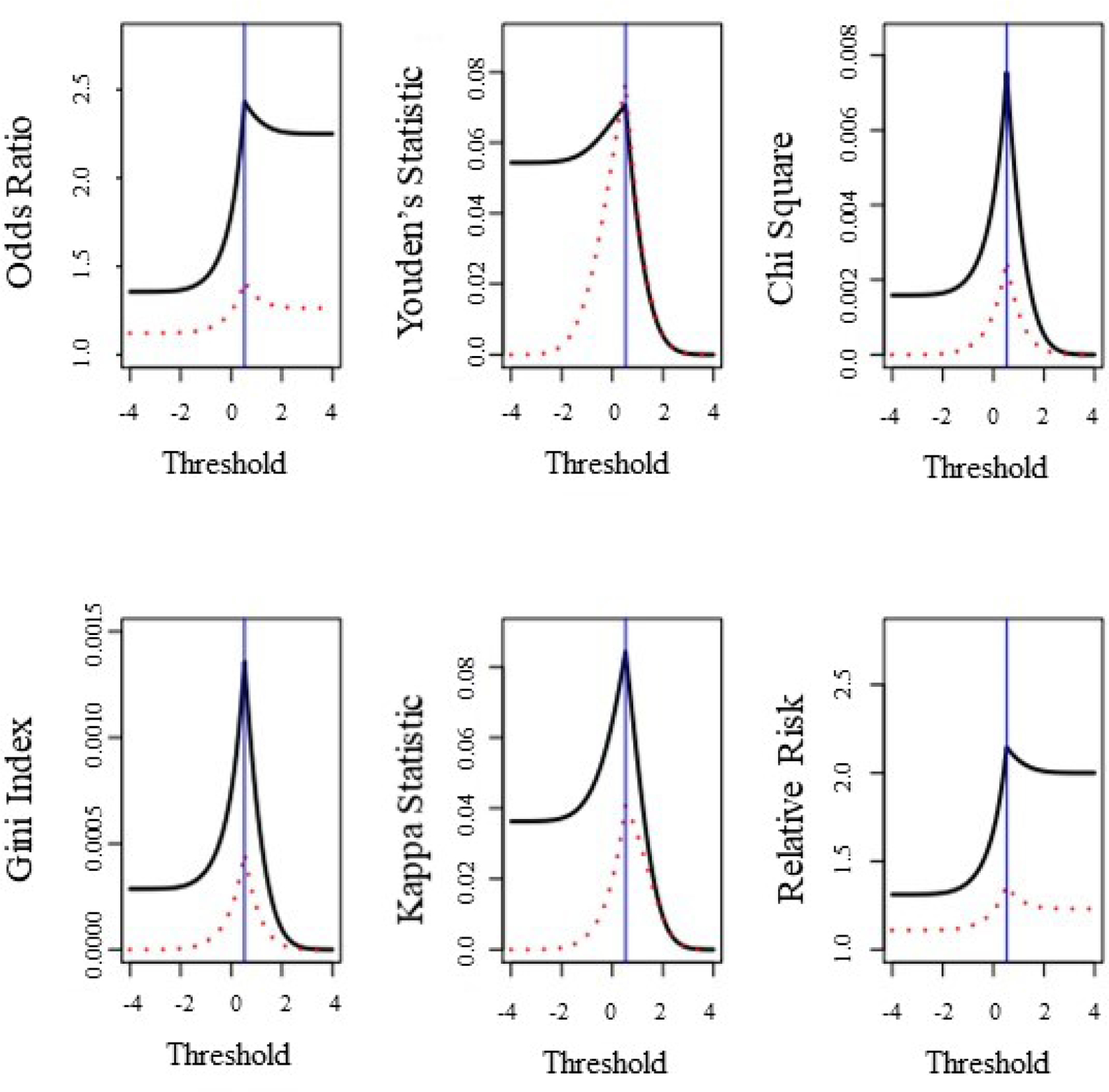
Values of statistics from Table 2 for different thresholds, $t_{x_1}$; for $X_1$ under single or joint thresholding in the case where two continuous variables $X_1$ and $X_2$ are associated with a binary outcome $Y$ the relationship in the Equation 2. Here $X~N_2\left(0,I_2\right),P_{X_1\ge T_1}>0.2,P_{X_2\ge T_2}>0.2,P_{Y=1}=0.2$, $P_{Y\mid T}=0.2$, and $P_{Y\mid F}=0.094$. The solid line represents the value of each statistic for values of $t_{x_1}$ in $[-\mathrm{4,4}]$ under joint thresholding where $t_{x_2}=T_2$. The dashed line represents the values of each statistic for values of $t_{x_1}$ under single thresholding. The vertical line occurs at the true threshold $T_1$ for $X_1$.

Figure 2:

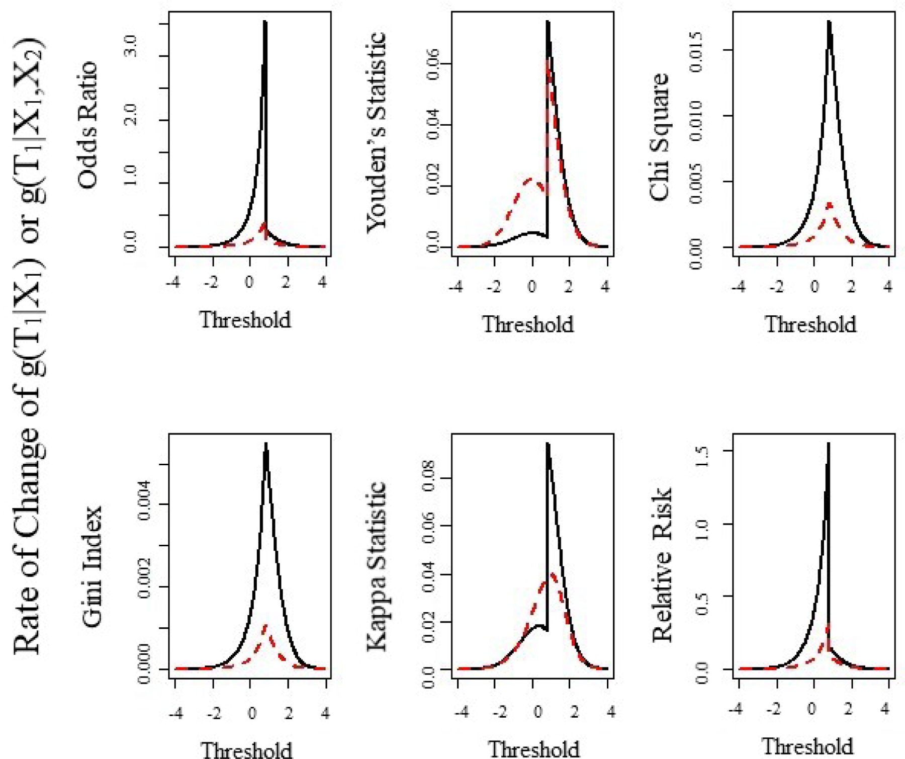
Numeric estimation of the first derivative of the six statistics from Table 2 for different values of threshold, $t_{x_1}$ for continuous variable $X_1$ under single or joint dichotomization. Here $P_{X_1\ge T_1}=0.2,P_{X_2\ge T_2}=0.2,P_{Y=1}=0.2$ and $OR=3$. Under joint dichotomization we assume that $t_{x_1}$ varies while $t_{x_2}=T_2$

In Figure 2, we examine the rate of change in $g\left(t_1\mid X_1\right)$ and $g\left(t_1\mid X_1,X_2\right)$ at $t_2=T_2$ for small changes in $t_1$. The rate of change is calculated for single thresholding as $g\left(t_{X_1}+0.001j_{X_1}\right)-g\left(t_{X_1}{j}_{X_1}\right)$ and for joint thresholding as $g\left(t_{X_1}+0.001j_{X_1},X_2\right)-g\left(t_{X_1}{j}_{X_1},X_2\right)$ for $t_{X_1}$ over the range $[-\mathrm{4,4}]$. The solid line is the rate of change under joint thresholding and the dashed line is the rate of change under single thresholding. For all six statistics in Table 2, the rate of change near $T_1$ is faster for joint thresholding relative to single thresholding. The plots of the derivatives (Figure 2) suggest, the rate of convergence to $T_1$ is faster for the odds ratio, relative risk, chi-square statistic, and gini index. With respect to the Youden’s and kappa statistics, the right convergence in faster to $T_1$ for joint versus single thresholding; however the left convergence is faster for single versus joint thresholding. We will comment about how this plays a role in estimating a threshold in our simulations.

3. Theoretical confirmation

Our previous work [12] demonstrated that dichotomization of a single variable based on the six statistics identify the correct threshold given one exists. Here we extend this work to the case of two continuous variables to discriminate a binary outcome $Y$. Consider two continuous variables $X_1$ and $X_2$ where the relationship between $X_1$ and $X_2$ with a dichotomous outcome $Y$ is defined by Equation 1. Define $g\left(T_1\mid X_1\right)$ and $g\left(T_2\mid X_2\right)$ as the functions for odds ratio, relative risk, chi-square statistic, gini index, Youden’s statistic, and kappa statistic under marginal thresholding of $X_1$ and $X_2$ respectively and $g\left(T_i\mid X_1,X_2\right),i=\mathrm{1,2}$ as the function for odds ratio, relative risk, chi-square statistic, gini index, Youden’s statistic, and kappa statistic for the $i^{\text{th}}$ threshold $(i=\mathrm{1,2})$ under joint thresholding of $X_1$ and $X_2$. Motivated by the numeric results in Section 2, we conjecture and prove the following theorems. Theorem 1 generalizes the results in Figure 1.

Theorem 1: For continuous variables $X_1$ and $X_2$ and a dichotomous variable $Y$ with prevalence $P_{Y=1}$ and thresholds $T_1$ and $T_2$ such that $P_{Y\mid \left(X_1\ge T_1,X_2\ge T_2\right)}>P_{Y\mid \left(X_1<T_{1}OR{X}_2<T_2\right)}$, (equation(1)), the inequality $g\left(t_1\mid X_1\right)<g\left(T_1\mid X_1\right)$ for any $t_1\ne T_1$ holds where $g\left(T_1\mid X_1\right)$ is any of the six statistics defined in Table 2. To consider the case where true thresholds exist, we assume for any $t_1\ne T_1$ that the conditional probability is a step function at $x_1>T_1$ and $x_2>T_2$.

We demonstrate the proof where $g\left(T_1\mid X_1\right)$ is the odds ratio and provide this proof in the supplemental material. The proof is under the assumption that $P_{Y\mid \left(X_1\ge T_1,X_2\ge T_2\right)}$ and the complement in the statement of the theorem are constant.

Next Theorem 2 generalizes the results of Figure 2 for any continuous $\mathbf{X}$ for odds ratio, relative risk, chi-square statistic, and gini index.

Theorem 2: For continuous variables $X_1$ and $X_2$ and a dichotomous variable $Y$ with prevalence $P(Y=1)$ and thresholds $T_1$ and $T_2$ such that $P_{Y\mid \left(X_1\ge T_1,X_2\ge T_2\right)}>P_{Y\mid \left(X_1<T_{1}OR{X}_2<T_2\right)}$ (Equation 2), the rate of convergence to $T_1$ is faster under joint compared to single thresholding. That is,

$$\frac{\partial g\left(T_1\mid X_1{X}_2\right)}{\partial T_1}>\frac{\partial g\left(T_1\mid X_1\right)}{\partial T_1},$$

when $g$ is one of statistics 1–4 in Table 2. This theorem can be stated in terms of $T_2$ as well.

This proof of Theorem 2 becomes trivial given the following lemma. Lemma 1 is also motivated by the results in Figure 1.

Lemma 1: For continuous variables $X_1$ and $X_2$ and a dichotomous variable $Y$ with prevalence $P(Y=1)$ and thresholds $T_1$ and $T_2$ such that $P_{Y\mid \left(X_1\ge T_1,X_2\ge T_2\right)}>P_{Y\mid {\left(X_1\ge T_1,X_2\ge T_2\right)}^c}$ then for functions $g$ defined earlier, $g\left(T_1\mid X_1,X_2\right)>g\left(T_1\mid X_1\right)$ where $g\left(T_1\mid X_1,X_2\right)$ is defined under joint thresholding using cell probabilities in Table 1 and $g\left(T_1\mid X_1,\right)$ is defined under single thresholding using the cell probabilities in a standard contingency table. We conjecture that this Lemma will extend to the case of $p$ continuous variables where the $p$ variables are associated with dichotomous outcome $Y$ through their interaction. This proof can be shown through induction.

Proof:

For the case where $g\left(t\right)$ is the odds ratio, the statement of the lemma is equivalent to the claim that

$$\frac{a_J{d}_J}{b_J{c}_J}>\frac{a_S{d}_S}{b_S{c}_S}$$

where $\left(a_S,b_S,c_S,d_S\right)$ are defined by the probabilities defined in a standard contingency table for the single thresholding case and $\left(a_J,b_J,c_J,d_J\right)$ are the cell probabilities for the joint thresholding case defined in Table 1 for the given thresholds $T_1$ and $T_2$. To prove the lemma, consider the inequality $P_{Y\mid T}>P_{Y\mid F}$ and multiply both sides by $P_{X_1\ge T_1,X_2<T_2}$ and $P_{X_1\ge T_1,X_2<T_2}=P_{X_1\ge T_1}-P_{X_1\ge T_1,X_2\ge T_2}$ which yields

$$P_{Y\mid T}\left(P_{X_1\ge T_1}-P_{X_1\ge T_1,X_2\ge T_2}\right)>P_{Y\mid F}{P}_{X_1\ge T_1,X_2<T_2}$$

Now adding $P_{Y\mid T}{P}_{X_1\ge T_1,X_2\ge T_2}-P_{Y\mid T}\left(P_{Y\mid T}{P}_{X_1\ge T_1,X_2\ge T_2}+P_{Y\mid F}{P}_{X_1\ge T_1,X_2<T_2}\right)$ to both sides and factoring and simplifying yields

$$\frac{P_{Y\mid T}}{\left(1-P_{Y\mid T}\right)}>\frac{P_{X_1\ge T_1,X_2\ge T_2}{P}_{Y\mid T}+P_{X_1\ge T_1,X_2<T_2}{P}_{Y\mid F}}{\left(P_{X_1\ge T_1}-P_{X_1\ge T_1,X_2\ge T_2}{P}_{Y\mid T}+P_{X_1\ge T_1,X_2<T_2}{P}_{Y\mid F}\right)}$$

Multiply both sides by $\frac{\left(1-P_{Y\mid F}\right)}{P_{Y\mid F}}$

$$\frac{P_{Y\mid T}\left(1-P_{Y\mid F}\right)}{\left(1-P_{Y\mid T}\right)P_{Y\mid F}}>\frac{P_{X_1\ge T_1,X_2\ge T_2}{P}_{Y\mid T}+P_{X_1\ge T_1,X_2<T_2}{P}_{Y\mid F}\left(1-P_{Y\mid F}\right)}{\left(P_{X_1\ge T_1}-P_{X_1\ge T_1,X_2\ge T_2}{P}_{Y\mid T}+P_{X_1\ge T_1,X_2<T_2}{P}_{Y\mid F}\right)P_{Y\mid F}}$$

Rearranging the terms and recognizing the factors yields

$$\frac{a_J{d}_J}{b_J{c}_J}>\frac{a_S{d}_S}{b_S{c}_S}$$

Thus,

$$O{R}_J>O{R}_S$$

Theorem 1 and Lemma 1 are also confirmed by the numeric findings shown in Figure 1. The proofs for Theorem 1 and Lemma 1 for Relative Risk, chi square, Kappa, Youden’s, and Gini Index can be found in Appendix B. Lemma 1 demonstrated that $g\left(T_i\mid X_1,X_2\right)>g\left(T_i\mid X_i\right)$ for $i=1$ or 2 and for all $T_1,T_2$ fixing $t_{X_i}=T_i$. Therefore, the proof of Theorem 2 follows. We demonstrate Theorem 2 further using a numeric approach shown in Figure 2. In Figure 2, we examine the rate of change in $g\left(t_{x_1}\mid X_1\right)$ and $g\left(t_{x_1}\mid X_1,X_2\right)$ at $t_{x_2}=T_2$ for small changes in $t_{X_1}$. The rate of change is calculated for single thresholding as $g\left(t_{X_1}+0.001\mid X_1\right)-g\left(t_{X_1}\mid X_1\right)$ and for joint thresholding as $g\left(t_{X_1}+0.001\mid X_1,X_2\right)-g\left(t_{X_1}\mid X_1,X_2\right)$ for $t_{X_1}$ over the range $[-\mathrm{4,4}]$. The solid line is the rate of change under joint thresholding and the dashed line is the rate of change under single thresholding. For all six statistics in Table 2, the rate of change near $T_1$ is faster for joint thresholding relative to single thresholding.

4. Joint thresholding algorithm

We propose an algorithm to jointly identify the best combination of thresholds $t_{x_1}$ and $t_{x_2}$ for $X_1$ and $X_2$ to discriminate a binary outcome $Y$. The proposed algorithm is shown in the box below.

In application it was noted that the six statistics were not stable when cell counts in the $2\times 2$ table were zero or small. Thus constraints on thresholds were applied. Specifically only values with 2 standard deviations of the means for $X_1$ and $X_2$ were considered for both the single and joint dichotomization algorithms.

5. Simulation Study

In sections 2 and 3, we demonstrated that the six statistics defined in Table 2 are maximized at the true threshold $\mathbf{T}$ when response $Y$ is associated with the continuous variables $X_1$ and $X_2$ through the relationship defined by Equation 2 whether $X_1$ and $X_2$ are dichotomized singly or jointly. Furthermore, we showed that joint dichotomization should converge to $T_1,T_2$ faster than single dichotomization for all six statistics if the relationship in Equation 2 is true. However, it is not generally known in advance whether or not $Y$ is associated with two continuous variables independently or through their interaction. Therefore, we investigate the ability of joint and single thresholding to recover the true thresholds, $T_1$ and $T_2$, for two continuous variables, $X_1$ and $X_2$, to discriminate a binary outcome $Y$ when $X_1$ and $X_2$ are associated with $Y$ when sampling from a population. A simulation study was conducted to evaluate the ability of the six statistics to correctly find $T_1$ and $T_2$ under different scenarios arising from combinations of (1) the relationship between $X={\left(X_1,X_2\right)}^{\prime }$ and $Y$ (independent or interaction), (2) strength of association between the predictors in $X$ and response $Y$ as defined by an odds ratio, and (3) value of the true thresholds $T_1$ and $T_2$.

Independent Case:

We set $P_{Y=1},P_{X_1}\ge T_1,P_{X_2}\ge T_2$, the odds ratio for $X_1\ge T_1,O{R}_1$, and the odds ratio for $X_2\ge T_2,O{R}_2$. In the case where the interaction, $X_1{X}_2$, is independently associated with $Y$, the OR is the product of $O{R}_1$ and $O{R}_2$. Continuous variables $X_1$ and $X_2$ are generated from $N_2~\left(0,I_2\right)$ and $T_1$ and $T_2$ are defined based on $P_{X_1\ge T_1}$ and $P_{X_2\ge T_2}$. The four probabilities, $P_1=P_{Y=1\mid X_1\ge T_1,X_2\ge T_2},P_2=P_{Y=1\mid X_1\ge T_1,X_2<T_2},P_3=P_{Y=1\mid X_1<T_1,X_2\ge T_2},P_4=P_{Y=1\mid X_1<T_1,X_2<T_2}$ can be calculated based on the set values of $T_1,T_2,O{R}_1$ and $O{R}_2$. Response $Y$ is generated from $\text{Bin} \left(n,P_k\right),k=1,\dots ,4$ based on the observed values of $X_1$ and $X_2$. For the independent case, we consider the scenarios outlined in Table 3 where probabilities $P_{X_1\ge T_1}$ and $P_{X_2\ge T_2}$ of 0.05, 0.2, and 0.5 yield thresholds of 1.645, 0.84, and 0 respectively.

Table 3:

Simulation Scenarios

OR	$P_{X_1\ge T_1}=P_{X_2\ge T_2}$	$P_{Y=1}$	Scenario
1.5	0.05	0.2	a
	0.2	0.2	b
	0.5	0.2	c
3	0.05	0.2	d
	0.2	0.2	e
	0.5	0.2	f
6	0.05	0.2	g
	0.2	0.2	h
	0.5	0.2	i

Joint case:

We set $P_{X_1\ge T_1},P_{X_2\ge T_2},P_{Y=1},P_{Y=1\mid X1\ge T1,X2\ge T2}$, and the OR for condition $X_1\ge T_1$ and $X_2\ge T_2$. Continuous variables $X_1$ and $X_2$ are generated from $N_2\left(0,I_2\right)$ and the true thresholds $T_1$ and $T_2$ are set as the inverse normal values of $P_{X_1>T_1}$ and $P_{X_2>T_2}$. Two probabilities $P_1=P_{Y=1\mid X_1\ge T_1,X_2\ge T_2}$ and $P_2=P_{Y=1\mid X_1\ge T_1\vee X_2\ge T_2}$ are calculated from the set values of $\text{OR},P_{Y=1},P_{X_1\ge T_1}$ and $P_{X_2\ge T_2}$,. Response $Y$ is generated from $\text{Bin} \left(n,P_w\right),w=1,\dots ,2$ based on the observed values of $X_1$ and $X_2$. For the joint case, we consider the scenarios outlined in Table 3 where probabilities $P_{X_1\ge T_1}=P_{X_2\ge T_2}$ of 0.05, 0.2, and 0.5 yield thresholds of 1.645, 0.84, and 0 respectively.

For each simulation scenario outlined in Table 3, we generated 500 datasets of sample size $n=\mathrm{100,250}$, and 500. The threshold for each method was estimated using the single and joint thresholding algorithms described in Section 3. The ability of each method to recover the true thresholds, $T_1$ and $T_2$, was evaluated by examining the mean squared error and the bias squared for the estimated threshold across all simulated datasets for all scenarios. All simulations were conducted in R v. 3.2.1 [13].

5.1. Simulation Results

Figures 3 and 4 show the results for thresholding $X_1$ singly and jointly. Each graph shows the mean squared error (MSE) by bias squared for all statistics described in Table 2 for the different values of $P_{X_1\ge T_1}$ and $P_{X_2\ge T_2}$ and strength of association with $Y$. The columns show the impact of increasing values for $P_{X_1\ge T_1}$ and $P_{X_2\ge T_2}$ and the rows show the impact of increasing strength of association with $Y$. Filled circles represent joint thresholding while open circles represent single. The columns in Figure 4 show the impact of increasing values for $P_{X_1\ge T_1}$ and $P_{X_2\ge T_2}$ and the rows show the impact of increasing strength of association with $Y$. Filled circles represent joint thresholding while open circles represent single thresholding. The results for thresholding $X_2$ were similar.

Figure 3:

The results from the simulation study comparing joint and single dichotomization of independent continuous variables. Each plot shows MSE by bias squared for the different values of $P_{X_1\ge T_1}$ and $P_{X_2\ge T_2}$ and strength of association with $Y$.

Figure 4:

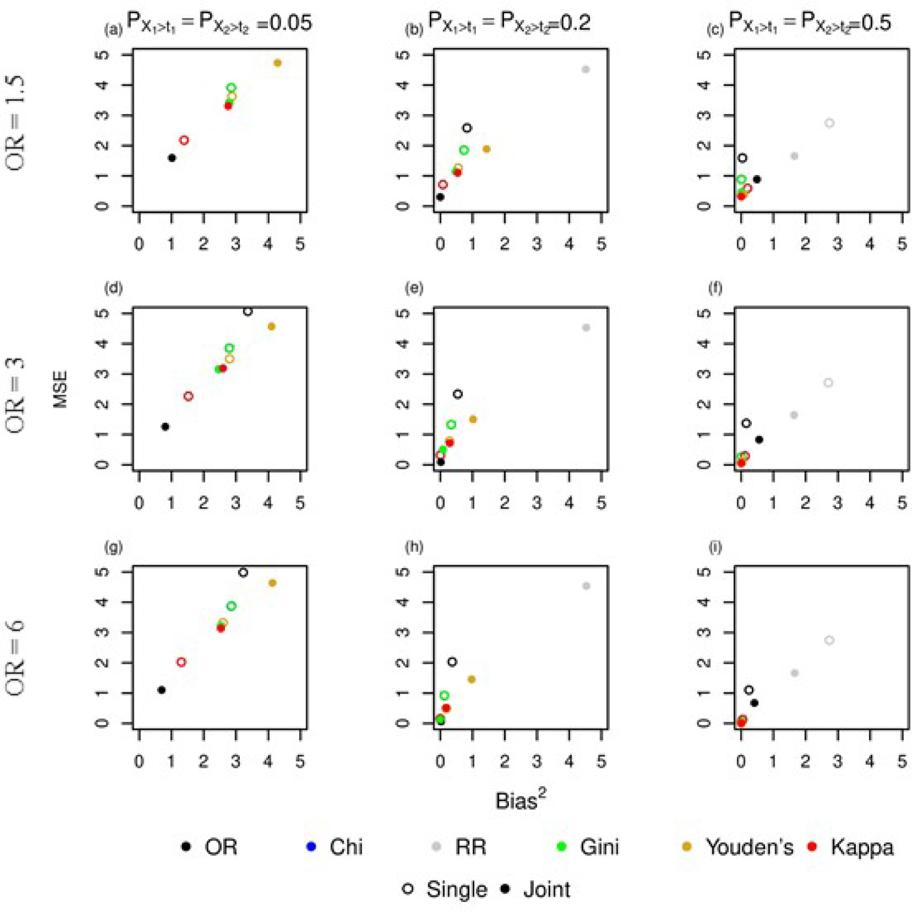
The results from the simulation study comparing joint and single dichotomization of interacting continuous variables. Each plot shows MSE by bias squared for the different values of $P_{X_1\ge T_1}$ and $P_{X_2\ge T_2}$ and strength of association with $Y$.

5.2. Independent case

In the independent case, as the strength of association between $X_1,X_2$ and $Y$ increases ($\text{OR}=1.5$ to $\text{OR}=6$), both joint and single thresholding exhibit smaller MSE for the estimated threshold for all methods and bias decreases slightly suggesting that the estimated threshold is less variable and biased as the strength of association between $X_1,X_2$ and $Y$ increases. When the strength of association is $\ge 3$, single thresholding is better for all methods except odds ratio and relative risk. Joint thresholding for kappa statistic has a lower MSE and bias than single thresholding for kappa when $P_{X_1\ge T_1}$ and $P_{X_2\ge T_2}$ increases to 0.5.

Holding odds ratio constant, as the probabilities $P_{X_1\ge T_1}$ and $P_{X_2\ge T_2}$ increase, both joint and single thresholding show a reduction in bias. At the lowest odds ratio $(\text{OR}=1.5)$ as $P_{X_1\ge T_1}$ and $P_{X_2\ge T_2}$ increase, the threshold estimated jointly using odds ratio, Gini Index, or relative risk has lower MSE and bias relative to the threshold selected using single thresholding. However, the jointly estimated threshold using Youden’s statistic or kappa statistic has higher bias and MSE than the threshold selected using single thresholding. When $P_{X_1\ge T_1}$ and $P_{X_2\ge T_2}=0.5$ (Figure 4c), selecting a threshold jointly based on kappa improves relative to single thresholding. Relative risk has the highest MSE and bias for both joint and single thresholding. Relative risk is not shown for plots 4a,d, and g due to the magnitude of the MSE and bias.

5.3. Joint Case

In the joint case, as the probability of observing values of $P_{X_1\ge T_1}$ and $P_{X_2\ge T_2}$ increase, both joint and single thresholding show a reduction in MSE and bias. As was seen in the independent case, selecting a threshold jointly using odds ratio, Gini Index, or relative risk result in a lower MSE and bias than single thresholding. However, the jointly estimated threshold using Youden’s statistic or kappa statistic has a higher MSE and bias than the threshold selected using single thresholding. When $P_{X_1\ge T_1}$ and $P_{X_2\ge T_2}=0.05$ or 0.2, selecting a threshold singly using kappa has a lower MSE and bias than jointly. But as the probability increases to $P_{X_1\ge T_1}$ and $P_{X_2\ge T_2}=0.5$, selecting a threshold jointly using kappa improves relative to single thresholding (Figures 4c,f, and i). When $P_{X_1\ge T_1}$ and $P_{X_2\ge T_2}=0.5$, single and joint thresholding using Youden’s statistic results in an MSE and bias approximately zero.

As the strength of association between $X_1,X_2$ and $Y$ increases ($\text{OR}=1.5$ to $\text{OR}=6$), both joint and single thresholding exhibit a reduction in MSE and bias decreases slightly suggesting that the estimated threshold is less variable and biased as the strength of association increases. Selecting a threshold jointly using odds ratio results in the lowest MSE and bias of all the methods except when $P_{X_1\ge T_1}$ and $P_{X_2\ge T_2}=0.5$. At this highest probability, selecting a threshold jointly and singly using chi square, gini index, Youden’s statistic and Kappa statistic result in a lower MSE and bias relative to joint thresholding using odds ratio. Single thresholding using relative risk results in the highest MSE and bias of all the methods.

5.4. Summary of Results

When $X_1$ and $X_2$ are independently associated with $Y$, single thresholding results in a lower MSE and bias when there is a weak association and small probability of observing values above a threshold. As that association and probability increase, joint thresholding performs similarly or better than single thresholding. When $X_1$ and $X_2$ are associated with $Y$ described by an interaction as described by Equation 2, joint thresholding with the odds ratio method results in the lowest MSE and bias when there is a weak or modest association with response variable $Y$. When there is a strong association and a high probability of observing values above a certain threshold, all of the methods except relative risk yield a low MSE and bias for the estimated thresholds. Results were similar across all sample sizes though MSE and bias increased with decreasing sample size (See Supplemental Material).

6. Conclusion

Previous research has shown that six of the common dichotomization methods work well in recovering a true threshold given our framework. This paper used those six dichotomization methods to recover the true threshold of two interacting variables. Identifying interactions that lead to increased risk of disease is an important step in understanding disease etiology. If two or more variables are dichotomized independently, their association with the outcome may never be identified. Thus, if continuous variables must be dichotomized and there is a suspected interaction, joint dichotomization is ideal. Even when two variables are independently associated with the outcome, joint dichotomization, particularly using the odds ratio, performs similarly or better than single dichotomization. Joint dichotomization is a first step in optimizing thresholds for 2 or more clinical predictors. Once the thresholds are selected, one could construct a hierarchical model using the selected thresholds to evaluate whether an interaction is statistically meaningful.

This paper provided mathematical and numeric proof that if $X_1$ and $X_2$ are associated with outcome through an interaction, joint dichotomization (1) yields a larger statistic for odds ratio, relative risk, chi square, Youden’s, Kappa and (2) converges more quickly to a true threshold $\text{T}$ than single thresholding. Through a simulation study, we showed that when a binary outcome is associated with two continuous variables through an interaction, dichotomizing them jointly to discriminate $Y$ recovers the true threshold with less variability than dichotomizing singly. Of the six statistics investigated, simulations showed that maximizing the odds ratio provided the most improvement when dichotomizing jointly instead of singly. In the proposed method, the region defined by the predictors is separated into two regions defined by the selected thresholds and therefore could easily be extended to more than two variables or cases where one predictor was continuous and another was binary.

In situations where interactions between variables are suspected and there is a need to dichotomize the continuous variables, these variables should be dichotomized jointly. However, our simulations showed that even in the independent case when $X_1$ and $X_2$ were associated with the outcome, joint thresholding was still shown to be effective in recovering a true threshold. In the case of the odds ratio statistic, joint thresholding performs better whether there is an interaction or not.

There are limitations to the method for joint dichotmization presented here. For example, we considered the case where true thresholds for the predictors exist. This is possible when disease outcome can be described by a mixture of normal distributions meaning disease negative has one distribution and disease positive has another distribution. However, dichotomies defined as in equation 2 are likely rare in real applications. Despite the ubiquitous use of dichotomization in clinical settings, statistical issues are well documented in the literature (Altman1994, MacCallum2002, Altman2006, Naggara2011). Specifically dichotomization can result in loss compromising power in testing hypotheses regarding the association of these predictors with the outcome (Metze2008). It may also lead to these associations being measured incorrectly (Hunter1990). Therefore, justification for dichotomizing needs to be addressed and we are exploring this in a subsequent paper. Additionally, the method assumes a continuous predictor has a dichotomous association with an outcome that is also dependent on another predictor, which should be verified.

7. Software

Software in the form of R code, together with a sample input data set and complete documentation is available on request from the corresponding author (sprincenelson@wlu.edu) and at Github

Box: Algorithm for jointly thresholding ${\mathit{X}}_1\mathbf{ }\mathbf{a}\mathbf{n}\mathbf{d}\mathbf{ }{\mathit{X}}_2$.

1. Order the values for each variable in $\mathbf{X}=\left(X_1,X_2\right)$, to yield $X=$ $\left(X_{\left(1\right)},X_{\left(2\right)}\right)$ which is the matrix $\mathbf{X}$ with values for $X_1$ and $X_2$ sorted in ascending order

2. Remove values that are not within two standard deviations of the mean.

3. For each pair $X_{\left(1_i\right)},X_{\left(2_j\right)}$ where $i,j=\mathrm{1,2},\dots ,n$, calculate the cell counts for a $2\times 2$ contingency table as follows:

   $$\begin{array}{l}{a}_{ij}=\sum _{k=1}^{n}I\left(X_{1k}\ge X_{\left(1i\right)}\right)\wedge I\left(X_{2k}\ge X_{\left(2j\right)}\right)\wedge I\left(Y_k=1\right)\\ b_{ij}=\sum _{k=1}^{n}I\left(X_{1k}\ge X_{\left(1i\right)}\right)\wedge I\left(X_{2k}\ge X_{\left(2j\right)}\right)\wedge I\left(Y_k=0\right)\\ c_{ij}=\sum _{k=1}^{n}I\left(X_{1k}<X_{\left(1i\right)}\right)\vee I\left(X_{2k}<X_{\left(2j\right)}\right)\wedge I\left(Y_k=1\right)\\ d_{ij}=\sum _{k=1}^{n}I\left(X_{1k}<X_{\left(1i\right)}\right)\vee I\left(X_{2k}<X_{\left(2j\right)}\right)\wedge I\left(Y_k=0\right)\end{array}$$ (6)
4. Select the pair $\left(X_{\left(1_i\right)},X_{\left(2_j\right)}\right)$ that maximizes the statistic $g\left(t\mid X_1,X_2\right)$, where $g\left(t\right)$ is one of the six statistics in Table 2. For example,

   $$O{R}_{ij}=\frac{a_{ij}{d}_{ij}}{b_{ij}{c}_{ij}}$$

References

- [1].Aoki K, Misumi J, Kimura T, Zhao W, Xie T, “Evaluation of Cutoff Levels for Screening of Gastric Cancer Using Serum Pepsinogens and Distributions of Levels of Serum Pepsinogen I, II and of PG I / PG II Ratios in a Gastric Cancer Case-Control Study”, Journal of Epidemiology volume 7, number 3, pages 143–151, (1997), DOI: 10.2188/jea.7.143 [DOI] [PubMed] [Google Scholar]
- [2].Benjamin O, Lappin SL “End-Stage Renal Disease”, StatPearls[Internet], 2021. Sep 16. Treasure Island (FL): StatPearls Publishing; 2021 Jan–. [PubMed] [Google Scholar]
- [3].Boehning D, Holling H, Patilea V, “ A limitation of the diagnostic-odds ratio in determining an optimal cut-off value for a continuous diagnostic test”, Statistical Methods in Medical Research, volume 20, number 5, pages 541–550, (2011) [DOI] [PubMed] [Google Scholar]
- [4].Breiman L, Friedman J, Stone CJ, Olshen RA, “ Classification and regression trees”, CRC press; (1984) [Google Scholar]
- [5].Greiner M, Pfeiffer D, Smith R.D.t, “ Principles and practical application of the receiver operating characteristic analysis for diagnostic tests”, Preventive Veterinary Medicine volume 45, pages 23–41, (2000) [DOI] [PubMed] [Google Scholar]
- [6].Greiner M, “Two-graph receiver operating characteristic (TG-ROC): a Microsoft-EXCEL template for the selection of cut-off values in diagnostic tests”, Journal of Immunological Methods, volume 185, number 1, pages 145–146, (1995) [DOI] [PubMed] [Google Scholar]
- [7].Kraemer HC, “ Risk ratios, odds ratio, and the test QROC. In: Evaluating medical tests”, pages 103–113, (1992), Newbury Park, CA: SAGE Publications, Inc [Google Scholar]
- [8].Lobo I, “Epistasis: Gene Interaction and the Phenotypic Expression of Complex Diseases Like Alzheimer’s,” Nature Education, 2008. 1(1):180. [Google Scholar]
- [9].Lopez-Raton M, Rodriguez-Alvarez MX, Cardosa-Suarez C, Gude-Sampedro F, “ OptimalCutpoints: An R package for selecting optimal cutpoints in diagnostic testing”, Journal of Statistical Software, volume 61, number 8, pages 1–36 (2014) [Google Scholar]
- [10].Manolio TA, Collins FS, “Genes, Enviornment, Health and Disease: Facing Up to Complexity”, Hum Hered 2007;63(2):63–6. doi: 10.1159/000099178 [DOI] [PubMed] [Google Scholar]
- [11].McKinney BA, Reif DM, Ritchie MD, Moore JH “Machine Learning for Detecting Gene-Gene Interactions” Applied Bioinformatics, 2006;5(2):77–88. doi: 10.2165/00822942-200605020-00002. [DOI] [PMC free article] [PubMed] [Google Scholar]
- [12].PrinceNelson SL, Ramakrishnan V, Nietert PJ, Kamen DL,Ramos PS, Wolf BJ, “An Evaluation of Common Methods for Dichotomization of Continuous Variables to Discriminate Disease Status,” Communication in Statistics, 2017; 46(21): 10823–10834 doi: 10.1080/03610926.2016.1248783. [DOI] [PMC free article] [PubMed] [Google Scholar]
- [13].R Core Team, “R:A Language and Environment for Statistical Computing”, R Foundation for Statistical Computing, 2013. Vienna, Austria. [Google Scholar]
- [14].SCORE2 working group and ESC Cardiovascular risk collaboration, “SCORE2 risk prediction algorithms: new models to estimate 10-year risk of cardiovascular disease in Europe,” European Heart Journal, volume 42, number 25, pages 2439–2454 (2021); doi: 10.1093/eurheartj/ehab309 [DOI] [PMC free article] [PubMed] [Google Scholar]
- [15].Strobl C, Boulesteix AL, Augustin T, “ Unbiased split selection for classification trees based on the Gini Index”, Computational Statistics and Data Analysis, volume 52, pages 483–501, (2007) [Google Scholar]
- [16].Tabor HK, Risch NJ, Myers RM, “Candidate-Gene Approaches for Studying Complex Genetic Traits: Practical Considerations”, Nature Reviews Genetics volume 3, pages391–397 (2002) 10.1038/nrg796 [DOI] [PubMed] [Google Scholar]
- [17].Vargha A, Rudas T,Delaney HD, Maxwell SE, “ Dichotomization, Partial Correlation, and Conditional Independence”, Journal of Educational and Behavioral Statistics, volume 21, number 3, pp. 264–282 (1996) 10.2307/1165272 [DOI] [Google Scholar]
- [18].Vermont J, Bosson JL, Francois P, Robert C, Rueff A, Demongeot J, “ Strategies for graphical threshold determination”, Computer Methods and Programs in Biomedicine, volume 35, pages 141–150, (1991) [DOI] [PubMed] [Google Scholar]
- [19].Youden WJ, “Index for rating diagnostic tests “, Cancer volume 3, number 1, pages 32–35 (1950) 10.1002/1097-0142(1950)3:1¡32::AID-CNCR2820030106¿3.0.CO;2-3 [DOI] [PubMed] [Google Scholar]
- [20].Altman DG, Lausen B, Sauerbrei W, Schumacher M, “Dangers of using “optimal” cutpoints in the evaluation of prognostic factors”, Journal of the National Cancer Institute, volume 86, number 11, pages 829–35,(1994). [DOI] [PubMed] [Google Scholar]
- [21].MacCallum R, Zhang S, Preacher K, “On the Practice of Dichotomization of Quantitative Variables”, Psychological Methods, volume 7, number 1, pages 19–40, (2002). [DOI] [PubMed] [Google Scholar]
- [22].Altman D, Royston P, “The cost of dichotomizing continuous variables”, British Medical Journal, volume 332, number 7549, pages 1080, (2006) [DOI] [PMC free article] [PubMed] [Google Scholar]
- [23].Naggara O, Raymond J, Guilbert F, Weill A, Altman DG, “Analysis by categorizing or dichotomizing continuous variables is inadvisable: an example from the natural history of unruptured aneurysms”, American Journal of Neuroradiology, volume 32, number 3, pages 437–40, (2011) [DOI] [PMC free article] [PubMed] [Google Scholar]
- [24].Metze K, “Dichotomization of continuous data– a pitfall in prognostic factor studies”, Pathology Research and Practice, volume 204, number 3, pages 213–214,(2008). [DOI] [PubMed] [Google Scholar]
- [25].Hunter J, Schmidt F, “Dichotomization of Continuous Variables: The Implications for Meta-Analysis”, Journal of Applied Psychology, volume 75, number 3, pages 334–49, (1990). [Google Scholar]
Associated Data
This section collects any data citations, data availability statements, or supplementary materials included in this article.