A Calibration Approach to Transportability and Data-Fusion with Observational Data

Summary

Two important considerations in clinical research studies are proper evaluations of internal and external validity. While randomized clinical trials can overcome several threats to internal validity, they may be prone to poor external validity. Conversely, large prospective observational studies sampled from a broadly generalizable population may be externally valid, yet susceptible to threats to internal validity, particularly confounding. Thus, methods that address confounding and enhance transportability of study results across populations are essential for internally and externally valid causal inference, respectively. These issues persist for another problem closely related to transportability known as data-fusion. We develop a calibration method to generate balancing weights that address confounding and sampling bias, thereby enabling valid estimation of the target population average treatment effect. We compare the calibration approach to two additional doubly-robust methods that estimate the effect of an intervention on an outcome within a second, possibly unrelated target population. The proposed methodologies can be extended to resolve data-fusion problems that seek to evaluate the effects of an intervention using data from two related studies sampled from different populations. A simulation study is conducted to demonstrate the advantages and similarities of the different techniques. We also test the performance of the calibration approach in a motivating real data example comparing whether the effect of biguanides versus sulfonylureas - the two most common oral diabetes medication classes for initial treatment - on all-cause mortality described in a historical cohort applies to a contemporary cohort of US Veterans with diabetes.

1 |. INTRODUCTION

Two common and related problems in statistics are causal inference and the generalizability of study results to a population of interest. A principal barrier to causal inference is mitigating confounding bias that can afflict the association between an exposure or treatment variable and the outcome. One solution for addressing confounding bias is to conduct a randomized trial. However, a randomized trial is impractical in many scientific and medical contexts. Therefore, methods for causal inference using observational data are essential. Even when valid causal inference can be drawn from a study, the effect estimates may not be accurate for the population of interest. This discordance occurs when the population that is sampled for an observational study or randomized trial - i.e. the study population - diverges from the specific population of interest for applying the study results – i.e. the target population. For example, the population of patients with a given disease may differ across important characteristics from the population receiving a specific intervention for that disease. In this simplistic scenario, extending valid inferences which evaluate the efficacy of the intervention to the target population containing every patient with the disease is of practical importance. For much of this manuscript, we focus on a more general yet well-defined setup for generalizing results onto a target population known as transportability.¹ Whereas generalizability requires the study population to be nested entirely within the target population, transportability allows the study and target populations to be disjoint. More information about the distinction between generalizability and transportability can be found elsewhere.^1,2 We then transition our attention to the problem of data-fusion,³ a closely related problem to transportability, wherein inferences occur on the target population and data for the outcome and treatment assignment are available from two respective samples of the target and study populations. Relative to transportability, where treatment and outcome data are only available for units in the study sample, the data-fusion estimator of a target population causal effect should be more efficient given the greater availability of data.

Methods for causal inference and transporting effect estimates to a target population are two recent topics of substantial interest in the statistical literature. Our goal is to combine methods found in these two respective areas in order to minimize bias due to confounding, which is unavoidable in observational studies, and to account for differences between study and target populations that could influence the causal effect estimate in the population of interest. The propensity score, or the probability of exposure given a set of measured covariates, has emerged as a popular tool in causal inference. Conditioning a causal effect estimator on the propensity score in essence balances the distribution of confounders between the exposed and unexposed participants in an observational study, thereby eliminating confounding bias.⁴ Through a similar mechanism, by conditioning a causal effect estimator on the sampling score, or the probability of being sampled for a study given the measured covariates, we can transport study results onto a target population in the presence of effect modification.¹ Extensions and comparisons of methods for transporting observational study results are limited, with most methods opting to focus on transporting results from a randomized controlled trial.^5,6,7,2 Moreover, there is little discussion on extensions for many of these methods to reconcile differences between two observational studies which examine the same exposure/outcome relationship, as in the data-fusion problem.³ Further compounding the issues already facing transportability and data-fusion, fitting parametric models of the propensity and sampling scores with maximum likelihood estimation has several limitations, particularly in finite sample settings. One of these issues is model misspecification.⁸ Therefore, the proposed implementations for extending inferences, either through transportability or data-fusion, should complement methodological developments found in the causal inference literature that overcome some of these limitations, such as double-robustness to help ameliorate model misspecification.

Calibration estimators⁹ have had recent success in both transporting causal effects from a randomized controlled trial to a target population and estimating causal effects using observational data. We propose combining the approach of Chan et al.¹⁰ and Josey et al.¹¹, which finds balancing weights that correct for confounding bias, with an exponential tilting estimator that estimates sampling weights to remove any bias attributable to differences in the covariate distribution between the study participants and non-participants sampled from the target population.¹² The exponential tilting approach to estimate sampling weights was used by Lee et al.⁶ to generalize randomized controlled trial results onto a target population characterized by an observational cohort. Their solution estimates the target population average treatment effect using a class of estimators that augment models for the propensity and sampling scores with a model of the outcome process.¹³ However, they stop short of identifying calibration weights that will also balance the covariate distribution between the treatment groups. To supplement their results, we propose a full calibration approach for transporting causal effects that produces weights that balance the covariate distribution between the treatment groups and between the study and target samples. We then show how the full calibration approach can be adapted to solve the data-fusion problem, enabling us to combine two observational studies that compare the same exposure and outcome. In the data-fusion setting, we will need to carefully consider additional assumptions appended to those already required for transportability. We demonstrate that the full calibration approach is doubly-robust, meaning that if either the potential outcome model is correctly specified or both the propensity and sampling score models are correctly specified, then the full calibration estimator of the target population average treatment effect is consistent.

To help showcase the proposed calibration solutions, we will evaluate effect estimates for diabetes treatment derived from older observational data on a contemporary real-world patient sample. This scenario is well-suited for transportability and data-fusion as diabetes patient characteristics, which potentially modify the effects of the initial diabetes treatments, have changed substantially over the last 10–20 years.^{14,15,16,17,18,19,20} The analysis here focuses on the comparative effectiveness of metformin and sulfonylureas - the two most commonly used drugs/classes for initial diabetes treatment in the US^21,22,23 - as first-line diabetes treatments. Several large observational studies and clinical trials comparing metformin and sulfonylureas have found that sulfonylurea use may be associated with poorer cardiovascular and mortality outcomes than metformin.^{24,25,26,27,28} Consequently, sulfonylurea use has declined over the last decade. However, they remain inexpensive and effective diabetes medications, making them an attractive treatment option in the right patients - for example, those at low risk of treatment related adverse events. With changing patient characteristics and more effective patient selection for sulfonylurea treatment, it is possible that the comparative effectiveness of sulfonylureas relative to metformin in real-world use has improved over time. We apply the transportability and data-fusion methods described in this manuscript to the problem of updating effect estimates of metformin versus sulfonylureas as a first-line diabetes treatment on all-cause mortality in the United States Veterans Affairs (VA) population. Using data available from 2004–2009, we will transport the risk difference of mortality from initial monotherapy with either a sulfonylurea or metformin regimen to a more contemporary cohort of diabetes patients diagnosed between 2010–2014. The estimated effects in the 2010–2014 sample will serve as a benchmark for the 2004–2009 cohort estimates transported to the 2010–2014 population. We also use the data-fusion approach to combine the 2004–2009 and 2010–2014 cohorts to estimate the treatment effect in the 2010–2014 VA diabetic population. Understanding how temporal changes in a health system’s patient population can modify the effect estimates from treatment choices for diabetes could have substantial population health impacts.

The remainder of this article is structured as follows. In Section 2 we introduce the notation and several assumptions that will be referenced throughout. In Section 3, we describe various methods for transporting causal effects in observational settings, including our proposed full calibration approach. In Section 4 we propose an extension to the full calibration method in Section 3 so that it is applicable in a data-fusion setting that requires combining observational studies. In Section 5, we compare the methods described in Sections 3 and 4 through simulations. Section 6 contains a data analysis using the full calibration approaches to transportability and data-fusion. Finally, we conclude with a discussion in Section 7.

2 |. SETTING AND PRELIMINARIES

2.1 |. Notation and Definitions

The setup for transportability and data-fusion with observational data requires - first and foremost - data from two separate observational studies. Define S_i ∈ {0, 1} as a sampling indicator denoting whether the independent sampling unit i = 1, 2, … , n is a study non-participant or participant. We sometimes refer to units {i : S_i = 1} as the study sample and units {i : S_i = 0} as the target sample. We denote $n_1={\sum }_{i=1}^n{S}_i$ and $n_0={\sum }_{i=1}^n\left(1-S_i\right)$ with n = n₁ + n₀. We suppose that the non-participants in the target sample represent a random sample from the target population - the population we would like to infer upon. The study sample is representative of the study population which is fundamentally different than the target population.

For each i = 1, 2, … , n, let ${\mathbf{X}}_i\in \mathcal{X}$ denote a vector of measured covariates, $Y_i\in \mathbf{\Re }$ denote the outcome and Z_i ∈ {0, 1} denote the treatment assignment. We apply the potential outcomes framework²⁹ to identify the causal estimand of interest and the necessary assumptions for transportability.³⁰ Let Y_i(0) denote the potential outcome when Z_i = 0 and Y_i(1) denote the potential outcome when Z_i = 1. The conditional expectations of these potential outcomes are denoted ${\mu }_0(\cdot )\equiv \mathbb{E}\left[Y_i(0)|\cdot \right]$ and ${\mu }_1(\cdot )\equiv \mathbb{E}\left[Y_i(1)|\cdot \right]$. The target population average treatment effect is defined as ${\tau }_0\equiv \mathbb{E}\left[Y_i(1)-Y_i(0)|S_i=0\right]$. τ₀ is the estimand of interest for both transportability and data-fusion.

Conditioned on X_i, we set ρ(X_i) ≡ Pr{S_i = 1|X_i}, π₁(X_i) ≡ Pr{Z_i = 1|S_i = 1, X_i} and π₀(X_i) ≡ Pr{Z_i = 1|S_i = 1, X_i} for all i = 1, 2, … , n. Note that the probability of treatment conditioned on the sample indicator and covariates can be alternatively expressed as

$${\pi }_s\left({\mathbf{X}}_i\right)\equiv \mathrm{Pr}\left\{Z_i=1|S_i=s,{\mathbf{X}}_i\right\}\equiv s{\pi }_1\left({\mathbf{X}}_i\right)+(1-s){\pi }_0\left({\mathbf{X}}_i\right).$$

Define {c_j (X) : j = 1, 2, …, m} as the set of functions that generate linearly independent features to be balanced between treatment groups and the two samples. We will refer to these quantities as balance functions. Furthermore, we will assume c₁(X_i) = 1 for all i = 1, 2, …, n. The target sample moments of the balance functions are defined as ${\widehat{\theta }}_{0j}=n_0^{-1}{\sum }_{i=1}^n\left(1-S_i\right)c_j\left({\mathbf{X}}_i\right)$, which is a consistent and unbiased estimator for ${\theta }_{0j}\equiv \mathbb{E}\left[c_j\left({\mathbf{X}}_i\right)|S_i=0\right]$ for all j = 1, 2, …, m. Finally, we define the logit link function as g(w) = log[w/(1 − w)] and its inverse g⁻¹(w) = exp(w)/[1 + exp(w)].

2.2 |. Assumptions for Transportability and Data-Fusion

2.2.1 |. Nonparametric Identifiability Assumptions

Under the potential outcomes model and given the definitions listed in the previous section, we may begin to develop the setting for which transportability and data-fusion methods are applicable using observational data.^31,3 We frame the setup to both problems through the following set of assumptions. These assumptions are an extension to those proposed in other articles regarding the transportability of experimental results across populations.^5,6 We combined these assumptions with the assumptions necessary for conducting causal inference in the presence of confounding.²⁹ To begin, we invoke the stable unit treatment value assumption which requires consistency, Y_i(z) = Y_i when Z_i = z, and no interference between units.²⁹ This means the observed outcome is equivalent to Y_i ≡ Z_iY_i(1) + (1 − Z_i)Y_i(0).

Assumption 1 (Strongly Ignorable Treatment Assignment).

In the case of transportability, the potential outcomes among the study participants are independent of the treatment assignment given X_i, and therefore: $\mathbb{E}\left[Y_i(z)|S_i=1,{\mathbf{X}}_i,Z_i\right]=\mathbb{E}[Y_i(z)|S_i=1,{\mathbf{X}}_i]$ for both z ∈ {0, 1}. For data-fusion, this condition is required for both study participants and non-participants: $\mathbb{E}\left[Y_i(z)|S_i,{\mathbf{X}}_i,Z_i\right]=\mathbb{E}\left[Y_i(z)|S_i,{\mathbf{X}}_i\right]$ for both z ∈ {0, 1}.

Assumption 2 (Treatment Effect Exchangeability).

Among all independent sampling units in either the study sample or the target sample, the expected value of the individual treatment effects conditioned on the covariates are exchangeable between samples: $\mathbb{E}\left[Y_i(1)-Y_i(0)|S_i,{\mathbf{X}}_i\right]=\mathbb{E}\left[Y_i(1)-Y_i(0)|{\mathbf{X}}_i\right]$ for all i = 1, 2, … , n.

Assumption 3 (Sample Positivity).

The probability of non-study participation, conditioned on the baseline covariates necessary to ensure treatment effect exchangeability, is bounded below by zero: Pr{S_i = 0|X_i} > 0 for all i = 1, 2, … , n.

Assumption 4 (Treatment Positivity).

For transportability, the probability of treatment conditioned on the baseline covariates in the study sample is bounded between zero and one: 0 < Pr{Z_i = 1|S_i = 1, X_i} < 1 for all i = 1, 2, … , n. For data-fusion, this condition is required for the both the study and target samples: 0 < Pr{Z_i = 1|S_i = 1, X_i} < 1.

2.2.2 |. Parametric Assumptions for Calibration Estimators

In addition to Assumptions 1–4, the following set of assumptions are necessary to establish the doubly-robust properties of the calibration weighted estimates for transportability and data-fusion. For more context, we will show that if either Assumption 5 is satisfied or both Assumptions 6 and 7 hold, then the so-called full calibration method that we present in Section 3.3 is consistent. If 6 and 7 hold, then 5 is not required to achieve statistical consistency. Likewise, if Assumption 5 holds then 6 and 7 are not required to ensure statistical consistency.

Assumption 5 (Conditional Linearity of the Potential Outcomes).

The expected value of the potential outcomes, conditioned on X_i, is linear across the span of the balancing functions while adhering to treatment effect exchangeability (Assumption 2):

$${\mu }_0\left(S_i=s,{\mathbf{X}}_i\right)=\sum _{j=1}^m{c}_j\left({\mathbf{X}}_i\right){\beta }_{sj}\text{and}{\mu }_1\left(S_i=s,{\mathbf{X}}_i\right)={\mu }_0\left(S_i=s,{\mathbf{X}}_i\right)+\sum _{j=1}^m{c}_j\left({\mathbf{X}}_i\right){\alpha }_j$$

for all i = 1, 2, … , n with ${\alpha }_j,{\beta }_{sj}\in \mathbf{\Re }$ for all i = 1, 2, … , m and s ∈ {0, 1}.

Assumption 6 (Conditional Linear Log-Odds for Sampling).

The log-odds of being in the study sample versus the target sample are linear across the span of the covariates: $g\left[\rho \left({\mathbf{X}}_i\right)\right]={\sum }_{j=1}^m{c}_j\left({\mathbf{X}}_i\right){\gamma }_j$ for all i = 1, 2, … , n and ${\gamma }_j\in \mathbf{\Re }$ for all i = 1, 2, … , m.

Assumption 7 (Conditional Linear Log-Odds for Treatment).

The probability of treatment in the study sample and the target sample are linear across the span of the covariates:

$$g\left[{\pi }_s\left({\mathbf{X}}_i\right)\right]=s\sum _{j=1}^m{c}_j\left({\mathbf{X}}_i\right){\lambda }_{1j}+(1-s)\sum _{j=1}^m{c}_j\left({\mathbf{X}}_i\right){\lambda }_{0j}$$

for all i = 1, 2, … , n and i = 1, 2, … , m with ${\lambda }_{0j},{\lambda }_{1j}\in \mathbf{\Re }$ and S_i = s.

The linearity conditions found in Assumptions 5–7 are relatively strong. Whereas the calibration estimators require the above representations of the potential outcome model, or the sampling and propensity scores, the alternative methods presented in Sections 3.1 and 3.2 have less stringent requirements to achieve statistical consistency. We will show that the targeted maximum likelihood approach makes the fewest parametric assumptions of all the methods that we will examine whereas the full calibration approach in Section 3.3 makes the most parametric assumptions for identification. Having fewer parametric assumptions allows for more intricate modeling choices, including the ability to employ machine learning techniques. However, these methods lose some interpretability provided by the calibration weights, which will exactly balance whichever distributional features are specified in the primal problem between the study and target samples and between the treatment groups - a quality often desired in causal analyses.³² While the TMLE and augmented approaches we present later on do not require parametric assumptions for identification, the methods used to estimate the nuisance parameters can be parametric. If the nuisance parameters are estimated with parametric models, then the TMLE and augmented approaches are also making the same strong parametric assumptions as the calibration approach. We demonstrate this fact in our simulation study in order to evaluate the doubly-robust properties of the various estimators outlined for τ₀.

2.2.3 |. Data-Fusion Specific Assumptions

The distinction between transportability and data-fusion essentially amounts to how much data we are provided from the study and target samples. For problems of transportability, we require the complete individual-level data from study sample, but only the individual-level covariate data from the target sample (i.e. X_i for all {i : S_i = 0}). In data-fusion, both the study and target samples provide data on X_i, Y_i, and Z_i for all i = 1, 2, … , n. It should not be a surprise that the latter setting is more powerful given the additional data. However, in many data analysis applications, Y_i and Z_i are not available from the target sample leaving data-fusion impracticable. In those cases, transportability is an appealing alternative.

Assumption 8 (Potential Outcome Exchangeability).

Among all independent sampling units in either the study or target sample, the expected value of the potential outcomes conditioned on the covariates are exchangeable between samples: $\mathbb{E}\left[Y_i(z)|S_i,{\mathbf{X}}_i\right]=\mathbb{E}\left[Y_i(z)|{\mathbf{X}}_i\right]$ for both z ∈ {0, 1}.

Assumption 9 (Propensity Score Exchangeability).

For all ${\mathbf{X}}_i\in \mathcal{X}$ we have π₁(X_i) = π₀(X_i).

The exchangeability assumptions of Assumptions 8 and 9 are key when considering the model design for estimators of τ₀ in the data-fusion setting. Potential outcome exchangeability is a stronger assumption than the assumptions of treatment effect exchangeability (Assumption 2). The former requires the expected values of the potential outcomes be exchangeable, conditional on the effect modifiers, confounders, and prognostic variables. We refer to prognostic variables as covariate measurements that are predictive of the outcome, but are otherwise uncorrelated with the treatment to be exclusive of confounders. The treatment effect exchangeability assumption, on the other hand, requires exchangeability conditional on both the effect modifiers to eliminate sampling bias and the confounders to eliminate confounding bias. Potential outcome exchangeability is a key limitation to more general approaches that impute potential outcomes for specific populations without necessarily evaluating a treatment effect.^33,34 Since comparable methods like the augmented approach⁶ and the target maximum likelihood approach⁵ that we will introduce in the next section require estimates of μ₀ (S_i, X_i) and μ₁ (S_i, X_i), potential outcome exchangeability becomes important if not necessary whenever both the study and target samples are used to estimate τ₀. Propensity score exchangeability assumes the propensity score is the same across both populations. This assumption is not an issue for transporting observational study results since these problems implicitly assume that the treatment assignment mechanism is the same for both samples. This is not an unreasonable assumption given that Z_i is not observed in the target sample in the transportability case. In the data-fusion setting, where the distribution of the treatment assignment can vary between samples, propensity score exchangeability becomes an important consideration. If both Assumptions 8 and 9 are violated, then S_i behaves like a surrogate confounder³⁵ and omitting it from either the potential outcome models or the propensity score model may lead to biased effect estimates.

3 |. METHODS FOR TRANSPORTING OBSERVATIONAL RESULTS

3.1 |. Targeted Maximum Likelihood

Targeted maximum likelihood estimation (TMLE) has emerged as a flexible framework for estimating a variety of causal estimands.³⁶ Specifically, Rudolph and van der Laan⁵ apply this framework to estimate τ₀ within the transportability setting described in Section 2.2. TMLE is adapted from the G-computation family of estimators which finds ${\widehat{\mu }}_0\left(S_i=1,{\mathbf{X}}_i\right)\equiv \widehat{\mathbb{E}}(Y_i|S_i=1,{\mathbf{X}}_i,Z_i=0)$ and ${\widehat{\mu }}_1\left(S_i=1,{\mathbf{X}}_i\right)\equiv \widehat{\mathbb{E}}\left(Y_i|S_i=1,{\mathbf{X}}_i,Z_i=1\right)$ using the independent sampling units {i : S_i = 1} to solve for

$${\widehat{\tau }}_{\text{G}}=\frac{1}{n_0}\sum _{\left\{i:S_i=0\right\}}\left[{\widehat{\mu }}_1\left(S_i=1,{\mathbf{X}}_i\right)-{\widehat{\mu }}_0\left(S_i=1,{\mathbf{X}}_i\right)\right].$$ (1)

For this estimator, if we can show ${\widehat{\mu }}_1\left(S_i=1,{\mathbf{X}}_i\right){\to }_p{\mu }_1\left(S_i=1,{\mathbf{X}}_i\right)$ and ${\widehat{\mu }}_0\left(S_i=1,{\mathbf{X}}_i\right){\to }_p{\mu }_0\left(S_i=1,{\mathbf{X}}_i\right)$, then given Assumptions 1–2 we have ${\widehat{\tau }}_G{\to }_p{\tau }_0$.

Rudolph and van der Laan⁵ extend this intuitive approach to account for potential bias induced from misspecifying ${\widehat{\mu }}_0(S_i=1,{\mathbf{X}}_i)$ and ${\widehat{\mu }}_1\left(S_i=1,{\mathbf{X}}_i\right)$. First, the proposed TMLE update will find estimates of the expected potential outcomes on the logit scale.³⁷ This requires standardizing $Y_i^{*}\equiv \left[Y_i-Y^{-}\right]{\left[Y^{+}-Y^{-}\right]}^{-1}$ where $Y^{-}\equiv {\min }_{\left\{i:S_i=1\right\}}\left(Y_i\right)$ and $Y^{+}\equiv {\max }_{\left\{i:S_i=1\right\}}\left(Y_i\right)$ from the available outcome data. Additionally, we will also need to find ${\widehat{\mu }}_0^{*}\left(S_i=1,{\mathbf{X}}_i\right)\equiv \widehat{\mathbb{E}}\left[Y_i^{*}|S_i=1,{\mathbf{X}}_i,Z_i=0\right]$ and ${\widehat{\mu }}_1^{*}\left(S_i=1,{\mathbf{X}}_i\right)\equiv \widehat{\mathbb{E}}\left[Y_i^{*}|S_i=1,{\mathbf{X}}_i,Z_i=1\right]$. The TMLE solution updates the estimates of the conditional means for the transformed potential outcomes using consistent estimates for ρ(X_i) and π₁(X_i), which we denote as $\widehat{\rho }\left({\mathbf{X}}_i\right)=\widehat{\mathrm{Pr}}\left\{S_i=1|{\mathbf{X}}_i\right\}$ and ${\widehat{\pi }}_1\left({\mathbf{X}}_i\right)\equiv \widehat{\mathrm{Pr}}\left\{Z_i=1|S_i=1,{\mathbf{X}}_i\right\}$. These estimators are combined into a so-called clever covariate³⁸ to find

$${\widehat{\eta }}_0^{*}\left(S_i=1,{\mathbf{X}}_i\right)=g^{-1}\left\{g\left[{\widehat{\mu }}_0^{*}\left(S_i=1,{\mathbf{X}}_i\right)\right]+{\widehat{ϵ}}_0\frac{\left[1-\widehat{\rho }\left({\mathbf{X}}_i\right)\right]}{\widehat{\rho }\left({\mathbf{X}}_i\right)\left[1-{\widehat{\pi }}_1\left({\mathbf{X}}_i\right)\right]}\right\}\text{and}$$

$${\widehat{\eta }}_1^{*}\left(S_i=1,{\mathbf{X}}_i\right)=g^{-1}\left\{g\left[{\widehat{\mu }}_1^{*}\left(S_i=1,{\mathbf{X}}_i\right)\right]+{\widehat{ϵ}}_1\frac{\left[1-\widehat{\rho }\left({\mathbf{X}}_i\right)\right]}{\widehat{\rho }\left({\mathbf{X}}_i\right){\widehat{\pi }}_1\left({\mathbf{X}}_i\right)}\right\}.$$

Estimates of the fluctuation coefficients $\widehat{ϵ}\equiv {\left({\widehat{ϵ}}_0,{\widehat{ϵ}}_1\right)}^T$ are found by projecting the transformed outcomes $Y_i^{*}$ onto the clever covariates

$${\widehat{h}}_0\left({\mathbf{X}}_i\right)=\frac{\left(1-Z_i\right)\left[1-\widehat{\rho }\left({\mathbf{X}}_i\right)\right]}{\widehat{\rho }\left({\mathbf{X}}_i\right)\left[1-{\widehat{\pi }}_1\left({\mathbf{X}}_i\right)\right]}\text{and}{\widehat{h}}_1\left({\mathbf{X}}_i\right)=\frac{Z_i\left[1-\widehat{\rho }\left({\mathbf{X}}_i\right)\right]}{\widehat{\rho }\left({\mathbf{X}}_i\right){\widehat{\pi }}_1\left({\mathbf{X}}_i\right)},$$

with $\widehat{\mathbf{h}}\left({\mathbf{X}}_i\right)\equiv {[{\widehat{h}}_0\left({\mathbf{X}}_i\right),{\widehat{h}}_1\left({\mathbf{X}}_i\right)]}^T$. In this regression, the initial estimates of the potential outcome means ${\widehat{\mu }}_0^{*}\left(S_i=1,{\mathbf{X}}_i\right)$ and ${\widehat{\mu }}_1^{*}\left(S_i=1,{\mathbf{X}}_i\right)$ serve as offsets. Analytically, estimates of the fluctuation coefficients $\widehat{ϵ}$ are found such that

$$\sum _{\left\{i:S_i=1\right\}}\widehat{\mathbf{h}}\left({\mathbf{X}}_i\right)\left(Y_i^{*}-g^{-1}\left\{Z_{i}g\left[{\widehat{\mu }}_1^{*}\left(S_i=1,{\mathbf{X}}_i\right)\right]+\left(1-Z_i\right)g\left[{\widehat{\mu }}_0^{*}\left(S_i=1,{\mathbf{X}}_i\right)\right]+{\widehat{\mathbf{h}}}^T\left({\mathbf{X}}_i\right)\widehat{ϵ}\right\}\right)=0.$$ (2)

Since this regression requires $Y_i^{*}$ and Z_i to be observed, estimates are calculated using the units {i : S_i = 1}. The TMLE estimate of τ₀ has a similar form to the G-computation setup, solving for

$${\widehat{\tau }}_{\text{TMLE}}=\frac{1}{n_0}\sum _{\left\{i:S_i=0\right\}}\left[{\widehat{\eta }}_1\left(S_i=1,{\mathbf{X}}_i\right)-{\widehat{\eta }}_0\left(S_i=1,{\mathbf{X}}_i\right)\right]$$ (3)

where ${\widehat{\eta }}_0\left(S_i=1,{\mathbf{X}}_i\right)=\left[Y^{+}-Y^{-}\right]{\widehat{\eta }}_0^{*}\left(S_i=1,{\mathbf{X}}_i\right)+Y^{-}$ and ${\widehat{\eta }}_1\left(S_i=1,{\mathbf{X}}_i\right)=\left[Y^{+}-Y^{-}\right]{\widehat{\eta }}_1^{*}\left(S_i=1,{\mathbf{X}}_i\right)+Y^{-}$. Given Assumptions 1–4, Rudolph and van der Laan⁵ show that the TMLE estimator for τ₀ is consistent if either the potential outcome models are consistent, or if $\widehat{\rho }\left({\mathbf{X}}_i\right){\to }_p\rho \left({\mathbf{X}}_i\right)$ and ${\widehat{\pi }}_1\left({\mathbf{X}}_i\right){\to }_p{\pi }_1\left({\mathbf{X}}_i\right)$. Gruber and van der Laan³⁷ argue that using the logit scale within TMLE constrains the fluctuation coefficients such that $Y^{-}\le {\widehat{\eta }}_0\left(S_i=1,{\mathbf{X}}_i\right)\le Y^{+}$ and $Y^{-}\le {\widehat{\eta }}_1\left(S_i=1,{\mathbf{X}}_i\right)\le Y^{+}$, thus avoiding extrapolations of the potential outcome mean estimates while retaining the doubly-robust properties inherent with TMLE.

3.2 |. Potential Outcome Model Augmentation

Another doubly-robust method for transporting causal effects is to augment the potential outcome model with weights derived from estimates of the propensity and sampling scores, similar to the implementation of the clever covariates used in TMLE.⁶ This method also builds upon the intuition surrounding the G-computation estimator found in (1). Below we present a brief summary of the augmented approach relevant for the transportability setting as opposed to the generalizability setting.² For a more complete description about how the method is applied in the generalizability setting, we suggest referring to the original text of Lee et al.⁶

The augmented approach proceeds by fitting component models of the data generating mechanisms for S_i, Y_i, and Z_i given Assumptions 1–4. While several estimators for the other nuisance parameters will suffice, the inverse odds of sampling are specifically estimated to satisfy the primal constrained optimization problem to

$$\begin{gathered} \mathrm{minimize}\sum _{\left\{i:S_i=1\right\}}\left\{q\left(S_i,{\mathbf{X}}_i\right)\log \left[q\left(S_i,{\mathbf{X}}_i\right)\right]-q\left(S_i,{\mathbf{X}}_i\right)\right\} \\ \text{subject}\text{to}\sum _{i=1}^n{S}_{i}q\left(S_i,{\mathbf{X}}_i\right)c_j\left({\mathbf{X}}_i\right)=n_1{\widehat{\theta }}_{0j}\text{for}\text{all}j=1,2,\dots ,m\text{.} \end{gathered}$$ (4)

Equation (4) can equivalently be solved with a Lagrangian dual problem which finds

$$\widehat{\mathit{\gamma }}=\underset{\mathit{\gamma }\in {\mathbf{\Re }}^m}{\arg \max }\sum _{\left\{i:S_i=1\right\}}\left\{-\exp \left[-S_i\sum _{j=1}^m{c}_j\left({\mathbf{X}}_i\right){\gamma }_j\right]-\sum _{j=1}^m{\widehat{\theta }}_{0j}{\gamma }_j\right\}$$ (5)

where $\widehat{\mathit{\gamma }}\equiv {\left({\widehat{\gamma }}_1,{\widehat{\gamma }}_2,\dots ,{\widehat{\gamma }}_m\right)}^T$. A Lagrangian dual is an unconstrained optimization problem derived by applying the Lagrangian multiplier theorem to a primal constrained convex optimization problem, like the one in (4). With the dual solution to (5), the resulting balancing weights that satisfy (4) can be found with

$$\widehat{q}\left(S_i,{\mathbf{X}}_i\right)=\exp \left[-S_i\sum _{j=1}^m{c}_j\left({\mathbf{X}}_i\right){\widehat{\gamma }}_j\right].$$ (6)

With the estimated sampling weights, the conditional mean estimates of the potential outcomes, and an appropriate propensity score model, Lee et al.⁶ construct an augmented estimator for τ₀ which solves for

$$\begin{gathered} {\widehat{\tau }}_{\text{AUG}}=\frac{1}{n_1}\sum _{\left\{i:S_i=1\right\}}\widehat{q}\left(S_i,{\mathbf{X}}_i\right)\left[\frac{Z_i\left[Y_i-{\widehat{\mu }}_1\left(S_i=1,{\mathbf{X}}_i\right)\right]}{{\widehat{\pi }}_1\left({\mathbf{X}}_i\right)}-\frac{\left(1-Z_i\right)\left[Y_i-{\widehat{\mu }}_0\left(S_i=1,{\mathbf{X}}_i\right)\right]}{1-{\widehat{\pi }}_1\left({\mathbf{X}}_i\right)}\right] \\ +\frac{1}{n_0}\sum _{\left\{i:S_i=0\right\}}\left[{\widehat{\mu }}_1\left(S_i=1,{\mathbf{X}}_i\right)-{\widehat{\mu }}_0\left(S_i=1,{\mathbf{X}}_i\right)\right]. \end{gathered}$$ (7)

The estimated inverse odds of sampling weights have the property that ${\sum }_{i=1}^n{S}_i\widehat{q}\left(S_i,{\mathbf{X}}_i\right)c_j\left({\mathbf{X}}_i\right)={\sum }_{i=1}^n\left(1-S_i\right)c_j\left({\mathbf{X}}_i\right)$ for all j = 1, 2, … , m. In other words, the weighted sample moments of the balance functions in the study sample are equal to the unweighted sample moments of the balance functions in the target sample. Under Assumptions 1–4, the augmented estimator ${\widehat{\tau }}_{\text{AUG}}$ can be shown to be doubly-robust.⁶ We can easily see this result given the following heuristic. In the scenario where ${\widehat{\mu }}_0\left(S_i=1,{\mathbf{X}}_i\right){\to }_p{\mu }_0\left(S_i=1,{\mathbf{X}}_i\right)$, ${\widehat{\mu }}_1\left(S_i=1,{\mathbf{X}}_i\right){\to }_p{\mu }_1\left(S_i=1,{\mathbf{X}}_i\right)$ the first summation in (7) has an expected value of zero while the second summation is consistent for τ₀. When Assumption 6 holds, if ${\widehat{\pi }}_1\left({\mathbf{X}}_i\right){\to }_p{\pi }_1\left({\mathbf{X}}_i\right)$, then the first sum in (7) will consistently negate the bias produced by the second summation.

3.3 |. A Full Calibration Approach to Transportability

Our proposed solution to the problem of transporting observational study results combines the calibration weighting approach for correcting confounding bias encountered within causal effect estimation¹¹ with the calibrated sampling weights used in Section 3.2, which removes bias induced by the differences of the covariate distribution between the two samples.^12,6 In other words, we estimate a vector of weights that concurrently balance both the samples and treatment groups.

The combined balancing and sampling weights are estimated contemporaneously in a manner similar to (5) and (6). The full calibration weights that balance both the treatment and sampling groups are estimated with the primal problem to

$$\begin{gathered} \text{minimize}\sum _{\left\{i:S_i=1\right\}}\left\{p\left(S_i,{\mathbf{X}}_i,Z_i\right)\log \left[p\left(S_i,{\mathbf{X}}_i,Z_i\right)\right]-p\left(S_i,{\mathbf{X}}_i,Z_i\right)\right\} \\ \text{subject}\text{to}\sum _{i=1}^n{S}_i\left(2Z_i-1\right)p\left(S_i,{\mathbf{X}}_i,Z_i\right)c_j\left({\mathbf{X}}_i\right)=0\text{(Propensity}\text{Score)} \\ \sum _{i=1}^n{S}_{i}p\left(S_i,{\mathbf{X}}_i,Z_i\right)c_j\left({\mathbf{X}}_i\right)=n_1{\widehat{\theta }}_{0j}(\text{Sampling}\text{Score}) \end{gathered}$$ (8)

for all j = 1, 2, … , m. Much like with the primal-dual relationship between (4) and (5), the primal problem in (8) can be equivalently solved by finding

$${\left({\hat{\mathit{\lambda }}}^T,{\hat{\mathit{\gamma }}}^T\right)}^T={\mathrm{argmax}}_{({\mathit{\lambda }}^T,{\mathit{\gamma }}^T{)}^T\in {\mathfrak{R}}^{2m}}\sum _{\{i:S_i=1\}}\left\{-\exp \left[-(2Z_i-1)\sum _{j=1}^m{c}_j\left({\mathbf{X}}_i\right){\lambda }_j-\sum _{j=1}^m{c}_j\left({\mathbf{X}}_i\right){\gamma }_j\right]-\sum _{j=1}^m{\hat{\theta }}_{0j}{\gamma }_j\right\}$$ (9)

where $\widehat{\mathit{\lambda }}\equiv {({\widehat{\lambda }}_1,{\widehat{\lambda }}_2,\dots ,{\widehat{\lambda }}_m)}^T$ which are then used to generate the balancing weights that satisfy (8) with

$$\widehat{p}\left(S_i,{\mathbf{X}}_i,Z_i\right)=\exp \left[-S_i\left(2Z_i-1\right)\sum _{j=1}^m{c}_j\left({\mathbf{X}}_i\right){\widehat{\lambda }}_j-S_i\sum _{j=1}^m{c}_j\left({\mathbf{X}}_i\right){\widehat{\gamma }}_j\right].$$ (10)

The desired estimand τ₀ is estimated using the Hajek-type estimator

$${\widehat{\tau }}_{\text{CAL}}=\frac{1}{n_1}\sum _{\left\{i:S_i=1\right\}}\widehat{p}\left(S_i,{\mathbf{X}}_i,Z_i\right)\left(2Z_i-1\right)Y_i.$$ (11)

The balancing weights from (10) achieve exact balance between the treatment-specific sample moments of the balance functions in the study sample and balances the balance function sample moments between the study and target samples. By rearranging the constraints of (8) we get

$$\sum _{i=1}^n{S}_i{Z}_i\widehat{p}\left(S_i,{\mathbf{X}}_i,Z_i\right)c_j\left({\mathbf{X}}_i\right)=\sum _{i=1}^n{S}_i\left(1-Z_i\right)\widehat{p}\left(S_i,{\mathbf{X}}_i,Z_i\right)c_j\left({\mathbf{X}}_i\right)=\frac{n_1{\widehat{\theta }}_{0j}}{2}.$$

Consequently, the estimator in (9)–(11) is equivalent to the estimator proposed in Josey et al.,² which was intended for transporting randomized experiments. Combining the results of the sampling and balancing weights allows us to apply M-estimation techniques to show that the double-robustness property holds under Assumption 5 or under the combination of Assumptions 6 and 7.³⁹ Additional details regarding modes of inference about τ₀ with ${\widehat{\tau }}_{\text{CAL}}$ can be found in the online supplement to Josey et al.²

4 |. A FULL CALIBRATION APPROACH FOR DATA-FUSION

There has been limited discussion in the literature on how the methods for transportability presented in Section 3 might be adapted for data-fusion. Recall that for the data-fusion setting, we are provided X_i, Y_i, and Z_i for all i = 1, … , n. The suggestion by Lee et al.⁶ is to use the outcome and treatment data from the target sample to find estimates ${\tilde{\mu }}_0\left(S_i=0,{\mathbf{X}}_i\right)\equiv \widehat{\mathbb{E}}[Y_i|S_i=0,{\mathbf{X}}_i,Z_i=0]$ and ${\tilde{\mu }}_1\left(S_i=0,{\mathbf{X}}_i\right)\equiv \widehat{\mathbb{E}}\left[Y_i|S_i=0,{\mathbf{X}}_i,Z_i=1\right]$, but otherwise keep the procedure in Section 3.2 the same. Invoking potential outcome exchangeability, we can find estimates of τ₀ by solving for

$$\begin{gathered} {\tilde{\tau }}_{\text{AUG}}=\frac{1}{n_1}\sum _{\left\{i:S_i=1\right\}}\widehat{q}\left(S_i,{\mathbf{X}}_i\right)\underset{\text{A}}{\underbrace{\{\frac{Z_i\left[Y_i-{\tilde{\mu }}_1\left(S_i=0,{\mathbf{X}}_i\right)\right]}{{\widehat{\pi }}_1\left({\mathbf{X}}_i\right)}}}-\underset{\text{B}}{\underbrace{\frac{\left(1-Z_i\right)\left[Y_i-{\tilde{\mu }}_0\left(S_i=0,{\mathbf{X}}_i\right)\right]}{1-{\widehat{\pi }}_1\left({\mathbf{X}}_i\right)}\}}} \\ +\frac{1}{n_0}\sum _{\left\{i:S_i=0\right\}}\underset{\text{C}}{\underbrace{\left[{\tilde{\mu }}_1\left(S_i=0,{\mathbf{X}}_i\right)-{\tilde{\mu }}_0\left(S_i=0,{\mathbf{X}}_i\right)\right]}} \end{gathered}$$ (12)

This simple modification to (7) implies that only units {i : S_i = 1} are used to de-bias estimates of the potential outcome means, assuming the potential outcome models are biased. The reasoning for not using all i = 1, 2, … , n for terms A and B of (12) is due to potential conflicts with propensity score exchangeability. Assuming potential outcome exchangeability holds but propensity score exchangeability is violated, then in order to use all available data to de-bias term C of (12) requires estimates of both π₀(X_i) in addition to π₁(X_i). This is because ${\widehat{\pi }}_1\left({\mathbf{X}}_i\right)$ would produce biased predictions from an incorrectly specified model of π₀(X_i). For now, the estimator in (12) does not require this assumption at the cost of losing a considerable degree of efficiency that a data-fusion estimator should otherwise gain. Even if specific models for π₁(X_i) and π₀(X_i) are fit in cases where propensity score exchangeability is violated, (12) is still subject to potential outcome exchangeability, unlike its transportability analogue. Let’s suppose that the outcome model is correctly specified for the target sample. If potential outcome exchangeability is violated, then terms A and B of (12) would likely introduce unchecked bias to ${\tilde{\tau }}_{\text{AUG}}$, even when the propensity score model of the study sample, ${\widehat{\pi }}_1\left({\mathbf{X}}_i\right)$, is correctly specified. This assumption could be counteracted in a similar way to counteracting violations to propensity score exchangeability – by fitting separate outcome models for the two samples and substituting them into (12) accordingly. Because of the extended exchangeability assumptions (Assumptions 8 and 9), the design decisions for data-fusion are more complex than the designs for transportability estimators.

We are intentional in constructing the full calibration data-fusion estimator such that it will not require either Assumptions 8 or 9 while still using all available data. To do this, ultimately, the full calibration approach to data-fusion will need to satisfy two additional constraints to balance treatment groups across both samples relative to the transportability approach in Section 3.3. This objective is not achieved by the primal problem in (8). The new goal is to estimate a set of dual vectors which can generate weights to balance the treatment groups while retaining the doubly-robust property. Once we estimate the new calibration weights, we can simply change the index of the summation in (11) to estimate τ₀ over all i = 1, 2, … , n.

For data-fusion, the primal problem of (8) is expanded upon to become

$$\begin{gathered} \mathrm{minimize}\sum _{i=1}^n\left\{p\left(S_i,{\mathbf{X}}_i,Z_i\right)\log \left[p\left(S_i,{\mathbf{X}}_i,Z_i\right)\right]-p\left(S_i,{\mathbf{X}}_i,Z_i\right)\right\} \\ \text{subject}\text{to}\sum _{i=1}^n{S}_i\left(2Z_i-1\right)p\left(S_i,{\mathbf{X}}_i,Z_i\right)c_j\left({\mathbf{X}}_i\right)=0(\text{Study}\text{Sample}\text{Propensity}\text{Score}), \\ \sum _{i=1}^n{S}_{i}p\left(S_i,{\mathbf{X}}_i,Z_i\right)c_j\left({\mathbf{X}}_i\right)=n_1{\widehat{\theta }}_{0j}(\text{Sampling}\text{Score}), \\ \sum _{i=1}^n\left(1-S_i\right)\left(2Z_i-1\right)p\left(S_i,{\mathbf{X}}_i,Z_i\right)c_j\left({\mathbf{X}}_i\right)=0,\text{(Target}\text{Sample}\text{Propensity}\text{Score)}, \\ \sum _{i=1}^n\left(1-S_i\right)p\left(S_i,{\mathbf{X}}_i,Z_i\right)c_j\left({\mathbf{X}}_i\right)=n_0{\widehat{\theta }}_{0j}\text{(Weight}\text{Stabilization)}, \end{gathered}$$ (13)

for all j = 1,2,...,m. Balancing the treatment specific moments in the study sample alone is not sufficient to also balance the treatment groups in the target sample that is required for data-fusion. For this reason, we added two extra constraints to the primal problem of (8) resulting in (13). Only the first three constraints would be required if we knew how to correctly specify the sampling and propensity scores, following Assumptions 6 and 7. The fourth constraint corrects the sampling variation from the target sample and is needed to ensure double-robustness when Assumption 5 holds. This constraint stabilizes the weights in the same way that the improved covariate balance propensity score formulation, thereby making the original proposal for the covariate balance propensity score estimator doubly-robust.⁴⁰ These constraints may be relaxed and altered further when the potential outcome exchangeability or the propensity score exchangeability assumptions are fulfilled. Careful attention should also be given to the size of the influence attributable to the respective samples after weighting. Note that the sum of the weights on the right hand side of the second and fourth equality constraints can be modified if more weight should be assigned to one sample versus the other.

Despite the changes to (8) expressed in (13), the primal-dual relationship is unaffected by the added constraints, barring any collinear balance functions. A new dual objective can be derived in the same manner as in Section 3.3 to find

$${\left({\tilde{\mathit{\lambda }}}_s^T,{\tilde{\mathit{\gamma }}}_s^T\right)}^T={\mathrm{argmax}}_{({\mathit{\lambda }}^T,{\mathit{\gamma }}^T{)}^T\in {\mathfrak{R}}^{2m}}\sum _{\{i:S_i=s\}}\left\{-\exp \left[-(2Z_i-1)\sum _{j=1}^m{c}_j\left({\mathbf{X}}_i\right){\lambda }_j-\sum _{j=1}^m{c}_j\left({\mathbf{X}}_i\right){\gamma }_j\right]-\sum _{j=1}^m{\hat{\theta }}_{0j}{\gamma }_j\right\}$$ (14)

where ${\widehat{\mathit{\lambda }}}_s\equiv {({\widehat{\lambda }}_{s1},{\widehat{\lambda }}_{s2},\dots ,{\widehat{\lambda }}_{sm})}^T$ and ${\widehat{\mathit{\gamma }}}_s\equiv {\left({\widehat{\gamma }}_{s1},{\widehat{\gamma }}_{s2},\dots ,{\widehat{\gamma }}_{sm}\right)}^T$ for s ∈ {0, 1}. The balancing weights combine the four estimated dual vectors to produce a solution to (13) with

$$\tilde{p}\left(S_i,{\mathbf{X}}_i,Z_i\right)=\exp \{-S_i\left[\left(2Z_i-1\right)\sum _{j=1}^m{c}_j\left({\mathbf{X}}_i\right){\widehat{\lambda }}_{1j}+\sum _{j=1}^m{c}_j\left({\mathbf{X}}_i\right){\widehat{\gamma }}_{1j}\right]-\left(1-S_i\right)\left[\left(2Z_i-1\right)\sum _{j=1}^m{c}_j\left({\mathbf{X}}_i\right){\widehat{\lambda }}_{0j}+\sum _{j=1}^m{c}_j\left({\mathbf{X}}_i\right){\widehat{\gamma }}_{0j}\right]\}.$$ (15)

The updated Hajek-estimator finds estimates of τ₀ by solving for

$${\tilde{\tau }}_{\text{CAL}}=\frac{1}{n}\sum _{i=1}^n\tilde{p}\left(S_i,{\mathbf{X}}_i,Z_i\right)\left(2Z_i-1\right)Y_i.$$ (16)

The summation in (16) uses all available data, i = 1, 2, … , n, meaning this estimator should be more efficient than the transportability proposal in (11). Neither the potential outcome exchangeability assumption nor the propensity score exchangeability assumption are necessarily required for the above approach, but they can be helpful to simplify some of the constraints in (13). This might be important in small sample settings where feasible solutions to (13) are difficult or impossible to achieve. For more information on how inference is conducted using this estimator, please refer to the online supplemental material.

5 |. SIMULATION STUDY

5.1 |. Simulation Setup

To demonstrate the efficacy of the different methods for transporting observational results, and to demonstrate the advantages of using data-fusion when it is feasible, we will conduct a simulation study that evaluates the performance of the three doubly-robust methods for transporting observational results that we have identified in Section 3 and the two data-fusion methods in Section 4. We will examine the performance of the proposed methodologies across a range of scenarios that test these methods when violations to the assumptions in Section 2.2 occur. To establish the doubly-robust quality of these estimators, we must consider possibilities where either the sampling and propensity score models are misspecified or the potential outcome models are misspecified. We also consider the sensitivity of these methods to practical violations to overlap. Finally, we examine the implications of Assumptions 8 and 9, which are particularly important for data-fusion. When potential outcome exchangeability holds but propensity score exchangeability does not, then S_i can be viewed as an instrumental variable as the sample indicator would affect the treatment assignment but would not have a direct impact on the outcome process that is not through the treatment assignment. Conversely, when propensity score exchangeability holds and potential outcome exchangeability is violated, then S_i is regarded as a nonconfounding prognostic variable in the sense that it predicts the outcome but does not confound the relationship between the treatment assignment and the outcome.

The scenarios we examine vary the sample size n ∈ {500, 1,000, 2,000}, the generative process that determines the treatment assignment through π_s(X_i), the potential outcome processes through μ₀(S_i, X_i) and μ₁(S_i, X_i), and the sampling mechanism ρ(X_i). These scenarios are detailed in Table 1. The covariate data X_i ≡ (X_i1, X_i2, X_i3, X_i4)^T are distributed as $X_{i1},X_{i2},X_{i3},X_{i4}~\mathcal{N}(0,1)$ for every i = 1, 2, … , n. We also generate the transformed variables U_i1 = exp[(X_i1 + X_i4)∕2], U_i2 = X_i2∕[1 + exp(X_i1)], U_i3 = log (|X_i2X_i3|), and U_i4 = (X_i3 + X_i4)² which are used in instances of model misspecification. Each entry in the vector U_i ≡ (U_i1, U_i2, U_i3, U_i4)^T is standardized to have a mean of zero and marginal variances of one - the same as for X_i. The sample indicators are generated assuming S_i ~ Bern ρ(X_i). Treatment assignments are generated by sampling from $Z_i~\mathrm{Bern}\left[{\pi }_{S_i}\left({\mathbf{X}}_i\right)\right]$. Finally, we generate the potential outcomes as $Y_i(0)~\mathcal{N}\left[{\mu }_0\left({\mathbf{X}}_i\cdot S_i\right),4\right]$ and $Y_i(1)~\mathcal{N}\left[{\mu }_1\left({\mathbf{X}}_i,S_i\right),4\right]$, which we use to generate the observed outcome Y_i = Z_iY_i(1) + (1 − Z_i)Y_i(0).

TABLE 1.

Simulation scenarios and the corresponding generative models for ρ(X_i), π_s(X_i), μ₀(X_t), and μ₁(X_i).

Exchangeability	Misspecification	Notes	Scenario	Data Generating Models
No Exchangeability Violation	No Model Misspecification	Baseline Example	A	$$\begin{gathered} g\left[\rho \left({\mathbf{X}}_i\right)\right]=0.5-0.5X_{i1}+0.5X_{i2}-0.5X_{i3}+0.5X_{i4} \\ g\left[{\pi }_{S_i}\left({\mathbf{X}}_i\right)\right]=0.5X_{i1}-0.5X_{i2}+0.5X_{i3}-0.5X_{i4} \\ {\mu }_0\left(S_i,{\mathbf{X}}_i\right)=2-3X_{i1}-X_{i2}+X_{i3}+3X_{i4} \\ {\mu }_1\left(S_i,{\mathbf{X}}_i\right)={\mu }_0\left(S_i,{\mathbf{X}}_i\right)-2-X_{i1}+3X_{i2}-3X_{i3}+X_{i4} \end{gathered}$$
	Outcome Model Misspecification	Sample Overlap Violation	B	$$\begin{gathered} g\left[\rho \left({\mathbf{X}}_i\right)\right]=2-2X_{i1}+2X_{i2}-2X_{i3}+2X_{i4} \\ g\left[{\pi }_{S_i}\left({\mathbf{X}}_i\right)\right]=0.5X_{i1}-0.5X_{i2}+0.5X_{i3}-0.5X_{i4} \\ {\mu }_0\left(S_i,{\mathbf{X}}_i\right)=2-3U_{i1}-U_{i2}+U_{i3}+3U_{i4} \\ {\mu }_1\left(S_i,{\mathbf{X}}_i\right)={\mu }_0\left(S_i,{\mathbf{X}}_i\right)-2-U_{i1}+3U_{i2}-3U_{i3}+U_{i4} \end{gathered}$$
		Treatment Overlap Violation	C	$$\begin{gathered} g\left[\rho \left({\mathbf{X}}_i\right)\right]=0.5-0.5X_{i1}+0.5X_{i2}-0.5X_{i3}+0.5X_{i4} \\ g\left[{\pi }_{S_i}\left({\mathbf{X}}_i\right)\right]=2X_{i1}-2X_{i2}+2X_{i3}-2X_{i4} \\ {\mu }_0\left(S_i,{\mathbf{X}}_i\right)=2-3U_{i1}-U_{i2}+U_{i3}+3U_{i4} \\ {\mu }_1\left(S_i,{\mathbf{X}}_i\right)={\mu }_0\left(S_i,{\mathbf{X}}_i\right)-2-U_{i1}+3U_{i2}-3U_{i3}+U_{i4} \end{gathered}$$
Potential Outcome Exchangeability Violation	Sampling and Propensity Score Misspecification	Prognostic Sampling Variable	D	$$\begin{gathered} g\left[\rho \left({\mathbf{X}}_i\right)\right]=0.5-0.5U_{i1}+0.5U_{i2}-0.5U_{i3}+0.5U_{i4} \\ g\left[{\pi }_{S_i}\left({\mathbf{X}}_i\right)\right]=0.5U_{i1}-0.5U_{i2}+0.5U_{i3}-0.5U_{i4} \\ {\mu }_0\left(S_i,{\mathbf{X}}_i\right)=S_i\left(2-3X_{i1}-X_{i2}+X_{i3}+3X_{i4}\right) \\ +\left(1-S_i\right)\left(2X_{i1}-2X_{i2}-2X_{i3}+2X_{i4}\right) \\ {\mu }_1\left(S_i,{\mathbf{X}}_i\right)={\mu }_0\left(S_i,{\mathbf{X}}_i\right)-2-X_{i1}+3X_{i2}-3X_{i3}+X_{i4} \end{gathered}$$
Propensity Score Exchangeability Violation	Outcome Model Misspecification	Instrumental Sampling Variable	E	$$\begin{gathered} g\left[\rho \left({\mathbf{X}}_i\right)\right]=0.5-0.5X_{i1}+0.5X_{i2}-0.5X_{i3}+0.5X_{i4} \\ g\left[{\pi }_{S_i}\left({\mathbf{X}}_i\right)\right]=S_i\left(0.5X_{i1}-0.5X_{i2}+2X_{i3}-2X_{i4}\right)-0.5\left(1-S_i\right) \\ {\mu }_0\left(S_i,{\mathbf{X}}_i\right)=2-3U_{i1}-U_{i2}+U_{i3}+3U_{i4} \\ {\mu }_1\left(S_i,{\mathbf{X}}_i\right)={\mu }_0\left(S_i,{\mathbf{X}}_i\right)-2-U_{i1}+3U_{i2}-3U_{i3}+U_{i4} \end{gathered}$$
Propensity Score and Potential Outcome Exchangeability Violation	No Model Misspecification	Confounding Sampling Variable	F	$$\begin{gathered} g\left[\rho \left({\mathbf{X}}_i\right)\right]=0.5-0.5X_{i1}+0.5X_{i2}-0.5X_{i3}+0.5X_{i4} \\ g\left[{\pi }_{S_i}\left({\mathbf{X}}_i\right)\right]=S_i\left(0.5X_{i1}-0.5X_{i2}+0.5X_{i3}-0.5X_{i4}\right)-0.5\left(1-S_i\right) \\ {\mu }_0\left(S_i,{\mathbf{X}}_i\right)=S_i\left(2-3X_{i1}-X_{i2}+X_{i3}+3X_{i4}\right) \\ +\left(1-S_i\right)\left(2X_{i1}-2X_{i2}-2X_{i3}+2X_{i4}\right) \\ {\mu }_1\left(S_i,{\mathbf{X}}_i\right)={\mu }_0\left(S_i,{\mathbf{X}}_i\right)-2-X_{i1}+3X_{i2}-3X_{i3}+X_{i4} \end{gathered}$$
	Sampling and Propensity Score Misspecification		G	$$\begin{gathered} g\left[\rho \left({\mathbf{X}}_i\right)\right]=0.5-0.5U_{i1}+0.5U_{i2}-0.5U_{i3}+0.5U_{i4} \\ g\left[{\pi }_{S_i}\left({\mathbf{X}}_i\right)\right]=S_i\left(0.5U_{i1}-0.5U_{i2}+0.5U_{i3}-0.5U_{i4}\right)-0.5\left(1-S_i\right) \\ {\mu }_0\left(S_i,{\mathbf{X}}_i\right)=S_i\left(2-3X_{i1}-X_{i2}+X_{i3}+3X_{i4}\right) \\ +\left(1-S_i\right)\left(2X_{i1}-2X_{i2}-2X_{i3}+2X_{i4}\right) \\ {\mu }_1\left(S_i,{\mathbf{X}}_i\right)={\mu }_0\left(S_i,{\mathbf{X}}_i\right)-2-X_{i1}+3X_{i2}-3X_{i3}+X_{i4} \end{gathered}$$
	Outcome Model Misspecification		H	$$\begin{gathered} g\left[\rho \left({\mathbf{X}}_i\right)\right]=0.5-0.5X_{i1}+0.5X_{i2}-0.5X_{i3}+0.5X_{i4} \\ g\left[{\pi }_{S_i}\left({\mathbf{X}}_i\right)\right]=S_i\left(0.5X_{i1}-0.5X_{i2}+0.5X_{i3}-0.5X_{i4}\right)-0.5\left(1-S_i\right) \\ {\mu }_0\left(S_i,{\mathbf{X}}_i\right)=S_i\left(2-3U_{i1}-U_{i2}+U_{i3}+3U_{i4}\right) \\ +\left(1-S_i\right)\left(2U_{i1}-2U_{i2}-2U_{i3}+2U_{i4}\right) \\ {\mu }_1\left(S_i,{\mathbf{X}}_i\right)={\mu }_0\left(S_i,{\mathbf{X}}_i\right)-2-U_{i1}+3U_{i2}-3U_{i3}+U_{i4} \end{gathered}$$

In the transportability examples, we will discard both Y_i and Z_i for all {i : S_i = 0}, and use only Y_i and Z_i from units {i : S_i = 1}. The data-fusion methods will make use of Y_i and Z_i for all i = 1, 2, … , n. Regardless of whether the method estimates τ₀ under the transportability case or the data-fusion case, each estimator is provided a design matrix containing an intercept term and the four original covariate measurements - X_i1, X_i2, X_i3, and X_i4 for all i = 1, 2, … , n. The target population average treatment effect is estimated across each iteration of a given scenario using the respective estimators described in Section 3: ${\widehat{\tau }}_{\text{TMLE}}$, ${\widehat{\tau }}_{\text{AUG}}$ and ${\widehat{\tau }}_{\text{CAL}}$. We also find estimates of τ₀ using the data-fusion estimators ${\tilde{\tau }}_{\text{AUG}}$ and ${\tilde{\tau }}_{\text{CAL}}$ from Section 4.

5.2. Simulation Results

We report the average bias and root mean square error (RMSE) for each of the scenarios described in Table 1 across 1,000 iterations using the estimators described in Sections 3 and 4. The results of the experiment are summarized in Table 2 for n = 500 and n = 2,000. Figure 1 provides a graphical representation of the results for n = 1,000. We also report the coverage probabilities in Table 3. The augmented and TMLE approaches use a plug-in estimator of the efficient influence function to find the 95% confidence intervals.⁵ For the full calibration approaches, the 95% confidence interval is estimated using a robust variance estimator.³⁹

TABLE 2.

Average Bias (RMSE) of the various Transportability and Data-Fusion estimators under several different simulation scenarios of the treatment assignment, sampling and outcome processes described in Table 1.

n	Scenario	τ 0	Transportability			Data-Fusion
			TMLE	AUG	CAL	AUG	CAL
500	A	−4.00	−0.01 (0.45)	0.00 (0.38)	−0.01 (0.36)	0.00 (0.38)	0.00 (0.32)
500	B	−3.51	2.73 (6.10)	0.38 (2.69)	1.95 (4.69)	0.37 (2.81)	2.70 (5.43)
500	C	−2.71	1.33 (5.50)	0.27 (1.61)	0.57 (2.54)	0.19 (1.73)	0.94 (3.50)
500	D	−2.73	−0.05 (0.37)	−0.01 (0.35)	−0.01 (0.35)	−0.27 (0.72)	−0.01 (0.33)
500	E	−2.71	−0.03 (0.95)	0.00 (0.83)	0.04 (0.72)	0.00 (0.86)	0.03 (0.50)
500	F	−4.00	0.02 (0.46)	0.01 (0.37)	0.02 (0.36)	0.03 (1.35)	0.01 (0.32)
500	G	−2.73	−0.03 (0.38)	0.01 (0.36)	0.01 (0.36)	−0.25 (0.70)	0.00 (0.34)
500	H	−2.71	−0.01 (1.02)	0.02 (0.83)	0.06 (0.78)	0.04 (1.11)	0.03 (0.54)
2000	A	−4.00	−0.01 (0.22)	0.00 (0.19)	0.00 (0.18)	0.00 (0.19)	0.00 (0.16)
2000	B	−3.51	0.85 (4.78)	0.09 (1.63)	0.25 (2.27)	0.06(1.67)	0.31 (2.25)
2000	C	−2.71	0.31 (4.59)	0.11 (1.09)	0.13 (0.92)	0.13 (1.32)	0.15 (0.67)
2000	D	−2.73	−0.04 (0.19)	0.00 (0.17)	0.00 (0.17)	−0.24 (0.39)	0.00 (0.17)
2000	E	−2.71	−0.04 (0.48)	−0.01 (0.46)	0.03 (0.38)	−0.01 (0.45)	0.01 (0.26)
2000	F	−4.00	−0.01 (0.21)	0.00 (0.19)	0.00 (0.18)	−0.01 (0.60)	0.00 (0.16)
2000	G	−2.73	−0.04 (0.20)	0.00 (0.19)	0.00 (0.19)	−0.26 (0.40)	0.00 (0.18)
2000	H	−2.71	−0.01 (0.47)	0.02 (0.43)	0.05 (0.38)	0.01 (0.65)	0.03 (0.26)

FIGURE 1.

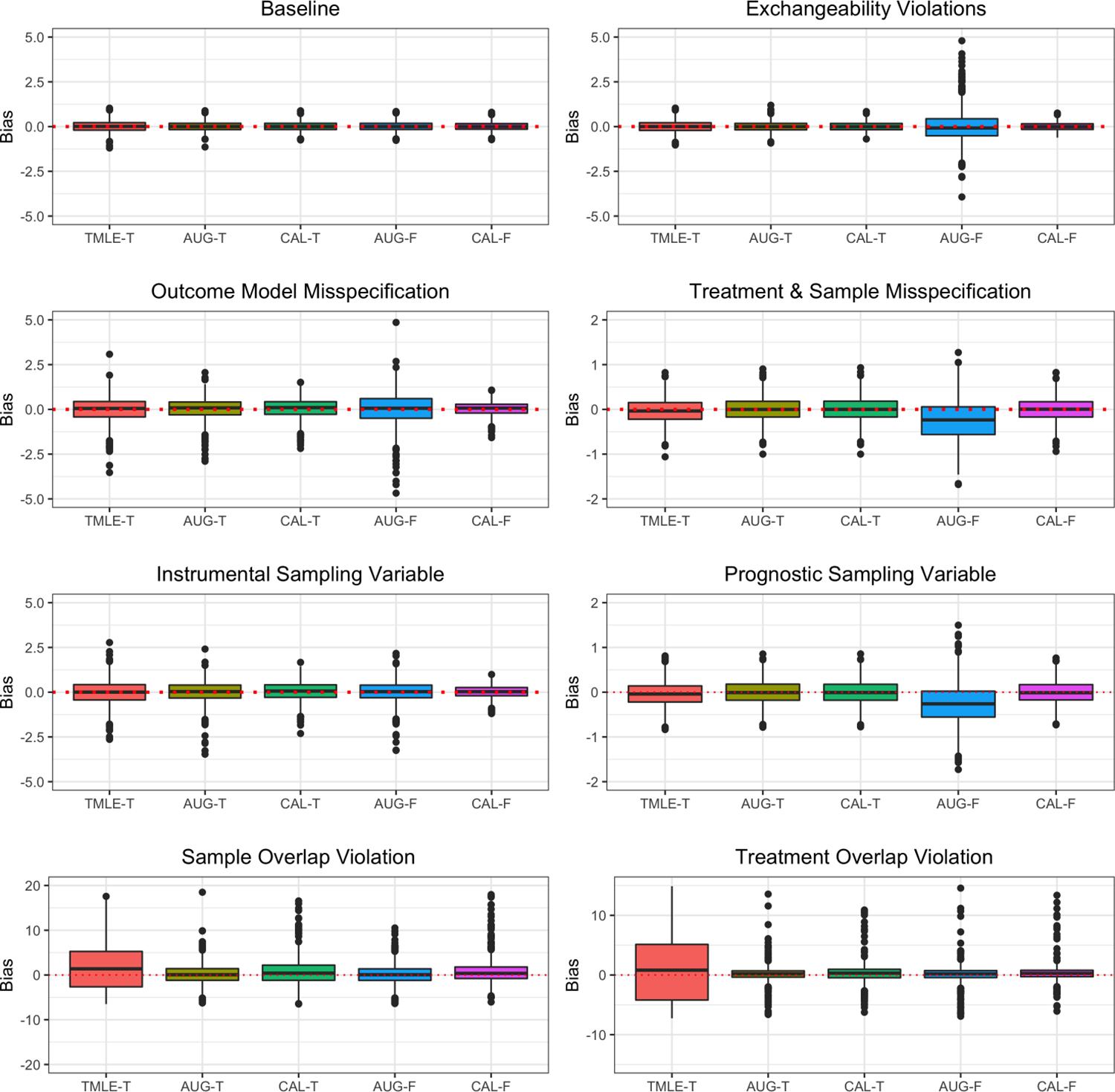
A subset of the constant conditional ATE estimates using four different methods for estimating balancing weights. Each boxplot is composed of 1,000 estimates from the replicates that generate the values in Table 2. The suffixes -T denotes the transportability case, while -F denotes the data-fusion case.

TABLE 3.

Coverage probabilities of τ₀ for the methods in Section 3 and 4.

n	Scenario	τ 0	Transportability			Data-Fusion
			TMLE	AUG	CAL	AUG	CAL
500	A	−4.00	0.946	0.946	0.929	0.954	0.940
500	B	−3.51	0.371	0.843	0.625	0.913	0.625
500	C	−2.71	0.134	0.898	0.690	0.903	0.694
500	D	−2.73	0.968	0.956	0.957	0.995	0.956
500	E	−2.71	0.899	0.952	0.927	0.976	0.951
500	F	−4.00	0.942	0.949	0.939	0.991	0.947
500	G	−2.73	0.970	0.958	0.960	0.993	0.957
500	H	−2.71	0.867	0.941	0.899	0.991	0.943
2000	A	−4.00	0.960	0.954	0.951	0.953	0.951
2000	B	−3.51	0.325	0.962	0.686	0.967	0.706
2000	C	−2.71	0.113	0.917	0.736	0.927	0.774
2000	D	−2.73	0.964	0.957	0.957	0.988	0.956
2000	E	−2.71	0.910	0.953	0.930	0.957	0.948
2000	F	−4.00	0.962	0.946	0.941	0.987	0.949
2000	G	−2.73	0.948	0.937	0.934	0.977	0.932
2000	H	−2.71	0.903	0.950	0.934	0.979	0.957

In the case of transportability, it is clear that the three methods from Section 3 perform equitably in scenarios where model misspecification occurs, and when there is some superseding exchangeability violation (Assumptions 8 and 9). The former scenarios demonstrate that each method is doubly-robust whereas the the latter scenarios make it abundantly clear that transportability is not affected by the potential outcome exchangeability assumption nor the propensity score exchangeability assumption. The full calibration approach achieved a lower RMSE whenever the outcome model was misspecified (Scenarios E and H). When the potential outcome models are correctly specified, the trade-offs between the different methods for transporting observational results are negligible. Regarding the scenarios with practical violations to overlap, it is apparent that the full calibration approach was less vulnerable in scenarios with treatment overlap violation (Scenario C) relative to the scenarios in which sample overlap is violated (Scenario B). The augmented approach achieved the least amount of bias in scenarios where there is limited sample overlap in terms of the average bias and the RMSE. When n = 500, the augmented approach performed better than the full calibration approach in scenarios where treatment group overlap was violated (Scenario C), but when n = 2,000 the degree of bias between the two methods is nearly identical. In this latter case, the full calibration approach had a smaller RMSE. Even though the full calibration approach performed worse than the augmented approach in scenarios involving a sample overlap violation, sample heterogeneity is still resolved using calibration thus marking the importance of this type of approach. This claim is further evidenced by the relatively poor results generated by the TMLE estimator in these settings. Furthermore, in Table 3, it appears that the full calibration approach retains accurate coverage probabilities of τ₀, whereas finding the 95% confidence interval with a plug-in estimator of the influence function sometimes overestimates the variance of the target population average treatment effect estimates.

When we combine datasets for data-fusion, we might expect to get more precise estimates of τ₀ than with an analogous transportability estimator. However, this is not the case for the data-fusion variant to the augmented approach. In many scenarios, the augmented estimator for data-fusion had a higher RMSE than the augmented estimator for transporting obbservational results. Recall that the proposed augmented solution has the same estimator in the data-fusion case as in the transportability case. The only difference between the two is the choice of initial outcome model. The only time that the RMSE is smaller was when some overlap violation occurs. The only occurrence where the full calibration approach to data-fusion was more accurate than the augmented approach concerning poor overlap conditions was when the treatment overlap assumption was violated (Scenario C) and n = 2,000. The same result occurs for the transportability case. Moreover, ${\tilde{\tau }}_{\text{AUG}}$ is biased whenever potential outcome exchangeability is violated and the propensity and sampling scores are incorrectly specified (Scenarios D and G), whereas the transportability variant of the augmented estimator is unbiased in these same scenarios. Once again, the coverage probabilities are accurate for the full calibration approach to data-fusion, yet the variance is over estimated for the augmented approach as seen in Table 3.

6 |. EVALUATING METFORMIN VERSUS SULFONYLUREAS AS MONOTHERAPY FOR VA DIABETES PATIENTS

The primary aim of this applied analysis is to estimate the risk difference in mortality between sulfonylurea and metformin monotherapy for the 2010–2014 cohort of diabetic VA patients. We first use improved covariate balance propensity score (CBPS) weights^40,11 to estimate the risk difference using only the 2010–2014 cohort, which balance the covariates found in Table 4. This estimate will serve as a benchmark for the transport and data-fusion settings. We also estimate the risk difference for the 2004–2009 cohort without the 2010–2014 data, again for comparative purposes. We use (9)–(11) to find estimates of total mortality in the 2004–2009 sample transported to the 2010–2014 cohort. Since sulfonylurea use in 2004–2009 represents 27.0% of monotherapy recipients but only 11.8% of patients in 2010–2014 implies the need for data-fusion methods which account for propensity score exchangeability violations, like that of the estimator in (14)–(16).

TABLE 4.

Summary statistics for covariates measured on newly diagnosed diabetic patients receiving care in the VA healthcare system stratified by years (2004–2009 and 2010–2014) and monotherapy type (Metformin or Sulfonylurea). The standardized absolute mean differences is an average measurement between the four temporal and treatment defined groups.

	Metformin (2004–2009)	Metformin (2010–2014)	Sulfonylurea (2004–2009)	Sulfonylurea (2010–2014)	Standardized Absolute Mean Difference
Patient Count	84003	100612	29447	11736	-
Baseline Age	61.90 (11.64)	60.45 (11.50)	67.32 (12.47)	66.95 (12.72)	0.354
Male	80964 (96.4)	95906 (95.3)	28912(98.2)	11472 (97.8)	0.095
Race/Ethnicity					0.185
Non-hispanic White	11927 (14.2)	20132 (20.0)	4038 (13.7)	2253 (19.2)
Non-hispanic Black	4730 (5.6)	6810(6.8)	1517 (5.2)	614 (5.2)
Hispanic	10897 (13.0)	8583 (8.5)	5073 (17.2)	1123 (9.6)
Other	56449 (67.2)	65087 (64.7)	18819 (63.9)	7746 (66.0)
Smoking Status					0.127
Current	21475 (25.6)	30603 (30.4)	6365 (21.6)	2925 (24.9)
Former	42751 (50.9)	44354 (44.1)	16396 (55.7)	5935 (50.6)
Never	19777 (23.5)	25655 (25.5)	6686 (22.7)	2876 (24.5)
BMI	32.96 (6.43)	33.66 (6.52)	31.20 (6.00)	32.08 (6.22)	0.220
SBP	133.03 (16.61)	132.35 (15.93)	133.83 (18.37)	131.80(17.31)	0.066
DBP	76.83 (10.82)	78.69 (10.76)	74.90 (11.59)	75.81 (11.45)	0.185
HDL	39.19 (10.76)	40.14 (10.97)	39.23 (11.51)	39.60(11.50)	0.048
LDL	103.43 (34.93)	102.68 (35.30)	101.32 (35.46)	96.99 (35.06)	0.098
Total Cholesterol	179.60(44.15)	178.57 (44.51)	177.91 (46.41)	173.49 (46.68)	0.069
Triglycerides	205.36 (192.15)	203.67 (198.23)	206.01 (198.88)	208.68 (216.49)	0.013
Fasting Plasma Glucose	151.54 (62.26)	149.71 (63.64)	165.87 (80.76)	163.67 (78.23)	0.141
HbA1c	7.17 (1.43)	7.28 (1.41)	7.42 (1.63)	7.54 (1.54)	0.139
Estimated GFR	78.41 (18.59)	83.88 (20.08)	66.83 (22.97)	66.15 (24.76)	0.500
Creatinine	1.03 (0.20)	0.98 (0.20)	1.25 (0.48)	1.29 (0.56)	0.493
History of CAD	31211 (37.2)	25771 (25.6)	14071 (47.8)	4535 (38.6)	0.240
History of CHF	8768 (10.4)	6086 (6.0)	5916 (20.1)	1752(14.9)	0.237
History of Stroke	10572(12.6)	8385 (8.3)	5230 (17.8)	1645 (14.0)	0.149
History of Kidney Disease	571 (0.7)	237 (0.2)	1214 (4.1)	316(2.7)	0.167
History of Liver Disease	424 (0.5)	349 (0.3)	278 (0.9)	86 (0.7)	0.043

Both cohorts excluded patients with pre-existing forms of cancer. We also omitted patients that received a second-line medication (either insulin, a thiazolidinedione, a sulfonylurea for patients receiving metformin, or metformin for patients receiving a sulfonylurea) within 30 days of their first filled prescription of either metformin or a sulfonylurea. Time to mortality, which is used to create the indicators of the three mortality outcomes, is computed as the number of days to death from the date when the first prescription is filled. Our analysis assumes intention to treat with the first prescribed therapy. We do not censor patients at the time when a second-line medication is prescribed, as was done in Wheeler et al.²⁶ The remaining baseline demographic and clinical characteristics about the two cohorts are summarized in Table 4.

Analyses based on covariate balance methods typically require checks to evaluate whether balance is actually achieved, both between the two samples and between the two treatment groups under investigation. A common diagnostic statistic for measuring balance is the standardized absolute mean difference evaluated over the various covariate measurements after weighting.³² We report this statistic for the unweighted differences in Table 4. With calibration, this step is redundant because the calibration weights should attain a standardized mean difference identical to zero (disregarding computational tolerance) in every feasible occasion (i.e. when a solution to the desired primal problem exists). However, it can still be helpful from a pedagogical standpoint to visualize this result. In the online supplement, we analyze a similar dataset comparing insulin sensitization therapy with insulin provisioning therapy for Type 2 diabetes patients – transporting and combining the results of the BARI 2D study⁴¹ with the 2010–2014 VA cohort. There we show a plot that illustrates the exact balancing nature of the calibration method, both between treatments and samples evaluated with the weighted standardized absolute mean differences. This supplemental analysis also provides an example for how we can combine experimental and observational datasets for data-fusion.

Another diagnostic is to compare the estimated propensity and sampling scores to ensure that there is sufficient overlap between the two treatment groups and between the two samples. We use a nonparametric kernel density estimator of the probability density function for the fitted propensity and sampling scores to visualize the degree that the treatment and sample stratified distributions overlap. Both the propensity score and the sampling score were fit using covariate balance propensity scores.⁴⁰ This diagnostic reveals the validity of the overlap assumptions (Assumptions 3 and 4). In Figure 2 we can see that there is indeed broad overlap between the sulfonylurea and metformin group, both in the 2004–2009 cohort and in the 2010–2014 cohort, and a considerable amount of overlap exists between samples based on the predicted sampling scores. Note that it is typically not possible to visualize the degree of overlap between treatments in the target sample under the transportability scenario, unless the treatment assignment is observed. Since our example works for both the transportability and data-fusion scenarios, we are able to estimate the propensity score in the target sample displayed in Figure 2.

FIGURE 2.

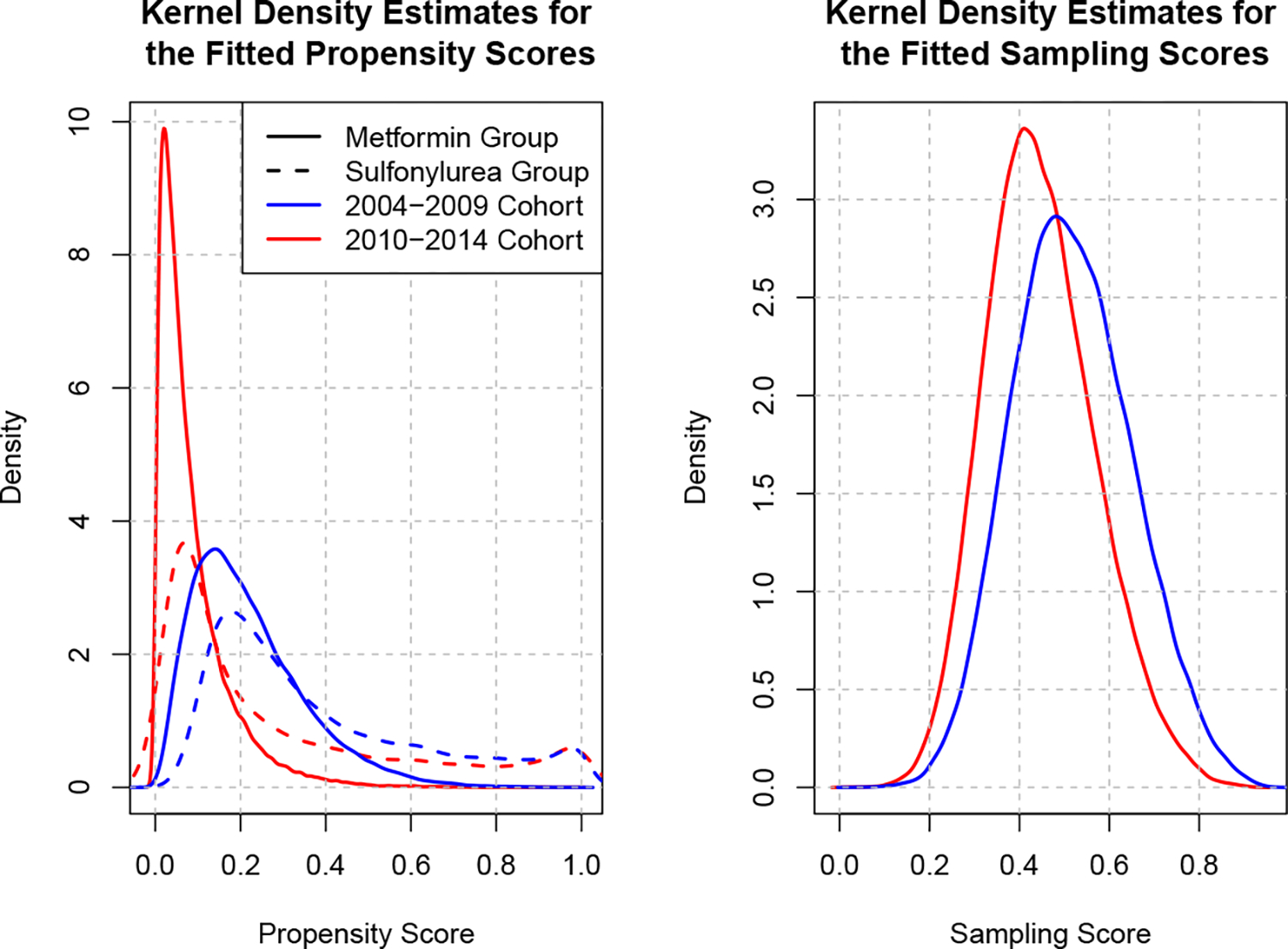
Kernel density estimates of the CBPS⁴⁰ fitted propensity and sampling scores. Recall that the propensity score measures the probability of being assigned to a sulfonylurea and the sampling score measures the probability of belonging to the 2004–2009 cohort versus the 2010–2014 cohort.

Table 5 contains the various risk-difference estimates that we computed on the illustrative dataset. We will primarily focus on the estimates of five-year mortality since these figures have the greatest magnitude. Furthermore, the trends that we will report about five-year mortality appear to be the same for one- and two-year mortality. Observe that the crude risk difference in five-year mortality is similar within both the 2004–2009 and in the 2010–2014 cohorts. This implies that there is either limited or no changes to the risk difference attributable to temporal trends in treatment effectiveness. Note that a temporal effect modifier is one factor that we would not be able to accommodate without violating sample positivity as it is collinear with the sample indicator. The adjusted marginal estimates of the risk difference using CBPS reveal the importance of accounting for differences observed between the study and target cohorts. The risk difference in the 2004–2009 cohort is 12.2%, 95% CI = (11.6%, 12.7%), and 4.1%, 95% CI = (3.4%, 4.9%), in the 2010–2014 cohort. Given the limited change of the crude estimates between cohorts, these discrepancies are likely due to differences in the distribution of effect modifiers between the two temporally-distinct cohorts. When we transport the estimates of the 2004–2009 cohort onto the 2010–2014 cohort, the risk difference is found to be 4.0%, 95% CI = (3.4%, 4.6%). That is, the transported effect estimate is more similar to the CBPS estimate of 2010–2014 than of the CBPS estimate evaluated on the 2004–2009 cohort. We also see that the transported estimate from the 2004–2009 cohort onto the 2010–2014 cohort is more efficient than the calibrated estimate computed with only the data from the 2010–2014 cohort.

TABLE 5.

Risk differences in total mortality between sulonylurea and metformin monotherapy in a VA cohort starting from the date of first prescription (Rx) using a variety of causal effect estimators.

Method and Sample	One Year after Rx	Two Years after Rx	Five Years after Rx
Unadjusted 2004–2009	2.6% (2.3%, 2.8%)	5.3% (4.9%,5.7%)	12.6% (11.9%, 13.2%)
Unadjusted 2010–2014	2.4% (2.0%, 2.7%)	5.1% (4.6%, 5.7%)	12.5% (11.7%, 13.4%)
CBPS 2004–2009	2.3% (2.1%, 2.6%)	5.0% (4.7%, 5.4%)	12.2% (11.6%, 12.7%)
CBPS 2010–2014	1.0% (0.7%, 1.4%)	2.0% (1.5%, 2.5%)	4.1% (3.4%, 4.9%)
Transported 2004–2009	0.8% (0.5%, 1.1%)	1.9% (1.4%, 2.3%)	4.0% (3.4%, 4.6%)
Data-Fusion	0.9% (0.7%, 1.1%)	2.1% (1.7%, 2.4%)	4.2% (3.7%, 4.7%)

We also examined the scenario which combines the 2004–2009 sample with the 2010–2014 sample to estimate the risk difference among patients in the 2010–2014 cohort using the extensions to (14)–(16) to accommodate the data-fusion setting. When we combine the two cohorts, we get an unbiased estimate of τ₀ with much greater efficiency than using only data from 2010–2014 alone. The efficiency gain is due to the increased effective sample size after weighting, which increased modestly from 30,883 in the transportability case to 37,682 in the data-fusion case. Using the data-fusion calibration estimator, we found the estimated risk difference for 2010–2014 to be 4.2%, 95% CI = (3.7%, 4.7%). Regardless of the estimator, our results suggest that metformin monotherapy remains associated with lower mortality than sulfonylurea treatment for veterans with newly-diagnosed diabetes. However, the size of the effect has declined over the two time periods, potentially implying improved patient selection for sulfonylurea treatment.

7 |. DISCUSSION

By estimating a vector of weights that simultaneously reduces sample and treatment group heterogeneity, we show how constrained convex optimization techniques can be applied to synergize solutions for causal inference using covariate balancing weights¹¹ with solutions for transporting experimental effect estimates using sampling weights.^12,1 The resulting estimator eliminates both confounding and sampling bias. This allows us to transport estimates found with observational data across populations. We also examined two alternative approaches for transporting experimental results which we adapted to accommodate data from observational studies. The TMLE⁵ and augmented estimators⁶ are less constrained by parametric assumptions, but their operational qualities are less interpretable if the desired objective is to balance covariate distributions between samples and treatment groups. We then demonstrate how the proposed full calibration approach can be extended to solve the problem of data-fusion in an observational context.

In the simulation study conducted in Section 5, we found that using some form of calibration, either with the augmented approach or the full calibration approach, yielded the most efficient estimates. In cases where the potential outcome models are correctly specified, the difference in performance between the three transportability estimators was negligible. For data-fusion, we saw in the simulation that the full calibration approach outperformed the alternative augmented approach. It is arguable that the increased efficiency might be the result of the implied parametric nature of the full calibration approaches. However, in this simulation, the nuisance parameters used by the TMLE and augmented estimators were fit using parametric models in an effort to better contrast the results. In addition to the simulation study, we show in an illustrative example evaluating mortality rates in US veterans with diabetes how different populations produce different effect estimates for the same outcome. We then demonstrate how eliminating the sampling bias induced by differences in the distribution of the effect modifiers between cohorts along with eliminating confounder heterogeneity between treatment groups produces consistent estimates of the treatment effect on the target population.

One of the major shortcomings of the full calibration method is the set of linearity conditions nested within Assumptions 5–7. These assumptions are necessary to guarantee the double-robustness property for this estimator. The TMLE approach does not require any assumption about the functional form of the nuisance parameters - the only requirement is that the nuisance parameter models be statistically consistent. The augmented approach as presented in Section 3.2 only requires Assumption 6, along with a statistically consistent propensity score, or consistent potential outcome models to guarantee double-robustness. In data-fusion, we show that Assumption 8 is required for the augmented approach in instances where the sampling and propensity scores are not correctly specified. We also note that the more stringent linearity assumptions culminate in a trade-off between more flexible modeling strategies and an increase to efficiency in finite sample settings, as demonstrated in the simulation study.

For much of this paper we have left the specification of the balancing weights c_j(X_i) to be ill-defined other than to set c₁(X_i) = 1 for all i = 1, 2, …, n. This latter property is necessary to stabilize the weights. Indeed, for many problems the choice of c_j(X_i) can simply be the original covariate measurements without any transformation, as we demonstrated in the simulations and illustrative examples. A more flexible yet complex option is to use sieve-type regression methods⁴² that replace the balance functions in the dual problems of (5), (9) and (14) with an expanding basis of functions and interactions among the covariate measurements. A sieve regression alternative would relax the linearity conditions in Assumptions 5–7. This nonparametric approach was explored in Chan et al.¹⁰ for estimating balancing weights to mitigate confounding bias and in Lee et al.⁶ for generalizing treatment effects.

In the case where we need to balance an exceptionally large number of balance functions, there is little to no assurance that a feasible solution to the primal problems in (4), (8) and (13) exists. To counteract this issue, we can introduce a penalization term on the dual variables in (5), (9) and (14). Doing so induces inequality constraints onto (4), (8) and (13), respectively, as opposed to the equality constraints that we currently solve. Introducing a penalization component, like in ridge regression or LASSO, results in a bias-variance trade-off in a finite sample setting. In finite sample settings without exact balance, estimates of τ₀ might be biased when using weights derived with penalization. However, a slightly biased estimate is certainly better than no estimate at all. Using such an approach was not necessary for either the simulation scenarios that we considered or for the illustrative examples, as these two applications are not high-dimensional cases. Using inequality constraints can also be used to reduce the mean squared error of an estimate for τ₀ if that is an objective of the analysis. More information on using inequality constraints with calibration can be found in Wang and Zubizarreta⁴³ for finding balancing weights and in Lu et al.⁴⁴ for transporting effect estimates.

Early on, we stated that the complete individual-level covariate data were required for both samples. It would be advantageous to only require the marginal moment values of the covariate distribution (or balance functions) in the target sample for transporting observational study results, as these entries are often found in the scientific and medical literature in a so-called Table 1. This setting is discussed in more detail by Josey et al.² for transporting randomized clinical trial results. In that article, we point out that any resulting inference in such a setting would involve the target sample average treatment effect, ${\tau }_0^{\prime }\equiv n_0^{-1}{\sum }_{\left\{i:S_i=0\right\}}{Y}_i(1)-Y_i(0)$, instead of the target population estimand of τ₀. The findings of Josey et al.² can easily be translated to the full calibration approach we propose for transporting observational results in Section 3.3 given that the two estimators of the target population average treatment effect are nearly identical. The augmented and TMLE approaches cannot be resolved in this context without additional assumptions given the need to sum the estimates of the potential outcome means over the target sample, which in general requires individual-level covariate data from the target sample. Given this finding, we believe calibration weights might be integrated or combined with the alternative estimators presented in this manuscript to further enhance these solutions when they are hindered by various modelling challenges, such as the setting where individual-participant study data are available but only marginal moment values of the target sample.

References

- 1.Westreich D, Edwards JK, Lesko CR, Stuart E, Cole SR. Transportability of trial results using inverse odds of sampling weights. American Journal of Epidemiology 2017; 186(8): 1010–1014. [DOI] [PMC free article] [PubMed] [Google Scholar]
- 2.Josey KP, Berkowitz SA, Ghosh D, Raghavan S. Transporting experimental results with entropy balancing. Statistics in Medicine 2021; 40(19): 4310–4326. [DOI] [PMC free article] [PubMed] [Google Scholar]
- 3.Bareinboim E, Pearl J. Causal inference and the data-fusion problem. Proceedings of the National Academy of Sciences 2016; 113(27): 7345–7352. [DOI] [PMC free article] [PubMed] [Google Scholar]
- 4.Rosenbaum PR, Rubin DB. The central role of the propensity score in observational studies for causal effects. Biometrika 1983; 70(1): 41–55. [Google Scholar]
- 5.Rudolph KE, van der Laan MJ. Robust estimation of encouragement design intervention effects transported across sites. Journal of the Royal Statistical Society: Series B (Statistical Methodology) 2017; 79(5): 1509–1525. [DOI] [PMC free article] [PubMed] [Google Scholar]
- 6.Lee D, Yang S, Dong L, Wang X, Zeng D, Cai J. Improving trial generalizability using observational studies. Biometrics 2021. [DOI] [PMC free article] [PubMed] [Google Scholar]
- 7.Dahabreh IJ, Robertson SE, Steingrimsson JA, Stuart EA, Hernán MA. Extending inferences from a randomized trial to a new target population. Statistics in Medicine 2020; 39(14): 1999–2014. [DOI] [PubMed] [Google Scholar]
- 8.Kang JDY, Schafer JL. Demystifying double robustness: a comparison of alternative strategies for estimating a population mean from incomplete data. Statistical Science 2007; 22(4): 523–539. [DOI] [PMC free article] [PubMed] [Google Scholar]
- 9.Deville JC, Särndal CE. Calibration estimators in survey sampling. Journal of the American Statistical Association 1992; 87(418): 376–382. [Google Scholar]
- 10.Chan KCG, Yam SCP, Zhang Z. Globally efficient non-parametric inference of average treatment effects by empirical balancing calibration weighting. Journal of the Royal Statistical Society. Series B, Statistical methodology 2016; 78(3): 673. [DOI] [PMC free article] [PubMed] [Google Scholar]
- 11.Josey KP, Juarez-Colunga E, Yang F, Ghosh D. A framework for covariate balance using Bregman distances. Scandinavian Journal of Statistics 2021; 48(3): 790–816. [Google Scholar]
- 12.Signorovitch JE, Wu EQ, Yu AP, et al. Comparative effectiveness without head-to-head trials. PharmacoEconomics 2010; 28(10): 935–945. [DOI] [PubMed] [Google Scholar]
- 13.Robins JM, Rotnitzky A, Zhao LP. Estimation of regression coefficients when some regressors are not always observed. Journal of the American Statistical Association 1994; 89: 846–866. [Google Scholar]
- 14.Ali MK, Bullard KM, Saaddine JB, Cowie CC, Imperatore G, Gregg EW. Achievement of goals in U.S. diabetes care, 1999–2010. The New England Journal of Medicine 2013; 368(17): 1613–1624. [DOI] [PubMed] [Google Scholar]
- 15.Selvin E, Parrinello CM, Sacks DB, Coresh J. Trends in prevalence and control of diabetes in the United States, 1988–1994 and 1999–2010. Annals of Internal Medicine 2014; 160(8): 517–525. [DOI] [PMC free article] [PubMed] [Google Scholar]
- 16.Gregg EW, Li Y, Wang J, et al. Changes in diabetes-related complications in the United States, 1990–2010. The New England Journal of Medicine 2014; 370(16): 1514–1523. [DOI] [PubMed] [Google Scholar]
- 17.Geiss LS, Wang J, Cheng YJ, et al. Prevalence and incidence trends for diagnosed diabetes among adults aged 20 to 79 years, United States, 1980–2012. JAMA 2014; 312(12): 1218–1226. [DOI] [PubMed] [Google Scholar]
- 18.Gregg EW, Cheng YJ, Srinivasan M, et al. Trends in cause-specific mortality among adults with and without diagnosed diabetes in the USA: an epidemiological analysis of linked national survey and vital statistics data. Lancet (London, England) 2018; 391(10138): 2430–2440. [DOI] [PubMed] [Google Scholar]
- 19.Cheng YJ, Imperatore G, Geiss LS, et al. Trends and disparities in cardiovascular mortality among U.S. adults with and without self-reported diabetes, 1988–2015. Diabetes Care 2018; 41(11): 2306–2315. [DOI] [PMC free article] [PubMed] [Google Scholar]
- 20.Raghavan S, Vassy JL, Ho YL, et al. Diabetes mellitus-related all-cause and cardiovascular mortality in a national cohort of adults. Journal of the American Heart Association 2019; 8(4): e011295. [DOI] [PMC free article] [PubMed] [Google Scholar]
- 21.Berkowitz SA, Krumme AA, Avorn J, et al. Initial choice of oral glucose-lowering medication for diabetes mellitus: a patient-centered comparative effectiveness study. JAMA internal medicine 2014; 174(12): 1955–1962. [DOI] [PubMed] [Google Scholar]
- 22.Hampp C, Borders-Hemphill V, Moeny DG, Wysowski DK. Use of antidiabetic drugs in the U.S., 2003–2012. Diabetes Care 2014; 37(5): 1367–1374. [DOI] [PubMed] [Google Scholar]
- 23.Desai NR, Shrank WH, Fischer MA, et al. Patterns of medication initiation in newly diagnosed diabetes mellitus: quality and cost implications. The American Journal of Medicine 2012; 125(3): 302.e1–7. [DOI] [PMC free article] [PubMed] [Google Scholar]
- 24.Schramm TK, Gislason GH, Vaag A, et al. Mortality and cardiovascular risk associated with different insulin secretagogues compared with metformin in type 2 diabetes, with or without a previous myocardial infarction: a nationwide study. European Heart Journal 2011; 32(15). [DOI] [PubMed] [Google Scholar]
- 25.Roumie CL, Hung AM, Greevy RA, et al. Comparative effectiveness of sulfonylurea and metformin monotherapy on cardiovascular events in type 2 diabetes mellitus: a cohort study. Annals of Internal Medicine 2012; 157(9): 601–610. [DOI] [PMC free article] [PubMed] [Google Scholar]
- 26.Wheeler S, Moore K, Forsberg CW, et al. Mortality among veterans with type 2 diabetes initiating metformin, sulfonylurea or rosiglitazone monotherapy. Diabetologia 2013; 56(9): 1934–1943. [DOI] [PubMed] [Google Scholar]
- 27.Hong J, Zhang Y, Lai S, et al. Effects of metformin versus glipizide on cardiovascular outcomes in patients with type 2 diabetes and coronary artery disease. Diabetes Care 2013; 36(5): 1304–1311. [DOI] [PMC free article] [PubMed] [Google Scholar]
- 28.Varvaki Rados D, Catani Pinto L, Reck Remonti L, Bauermann Leitão C, Gross JL. The association between sulfonylurea use and all-cause and cardiovascular mortality: a meta-analysis with trial sequential analysis of randomized clinical trials. PLoS medicine 2016; 13(4): e1001992. [DOI] [PMC free article] [PubMed] [Google Scholar]
- 29.Rubin DB. Estimating causal effects of treatments in randomized and nonrandomized studies.. Journal of Educational Psychology 1974; 66(5): 688. [Google Scholar]
- 30.Lesko CR, Buchanan AL, Westreich D, Edwards JK, Hudgens MG, Cole SR. Generalizing study results: a potential outcomes perspective. Epidemiology (Cambridge, Mass.) 2017; 28(4): 553–561. [DOI] [PMC free article] [PubMed] [Google Scholar]
- 31.Pearl J, Bareinboim E. External validity: from do-calculus to transportability across populations. Statistical Science 2014; 29(4): 579–595. [Google Scholar]
- 32.Austin PC. Balance diagnostics for comparing the distribution of baseline covariates between treatment groups in propensity-score matched samples. Statistics in Medicine 2009; 28(25): 3083–3107. [DOI] [PMC free article] [PubMed] [Google Scholar]
- 33.Keele L, Ben-Michael E, Feller A, Kelz R, Miratrix L. Hospital Quality Risk Standardization via Approximate Balancing Weights. arXiv preprint arXiv:2007.09056 2020. [Google Scholar]
- 34.Hirshberg DA, Maleki A, Zubizarreta JR. Minimax linear estimation of the retargeted mean. arXiv preprint arXiv:1901.10296 2019. [Google Scholar]
- 35.VanderWeele TJ, Shpitser I. On the definition of a confounder. Annals of Statistics 2013; 41(1): 196. [DOI] [PMC free article] [PubMed] [Google Scholar]
- 36.van der Laan MJ, Rubin D. Targeted maximum likelihood learning. The International Journal of Biostatistics 2006; 2(1). [DOI] [PMC free article] [PubMed] [Google Scholar]
- 37.Gruber S, van der Laan MJ. A targeted maximum likelihood estimator of a causal effect on a bounded continuous outcome. The International Journal of Biostatistics 2010; 6(1). [DOI] [PMC free article] [PubMed] [Google Scholar]
- 38.Schuler MS, Rose S. Targeted maximum likelihood estimation for causal inference in observational studies. American Journal of Epidemiology 2017; 185(1): 65–73. [DOI] [PubMed] [Google Scholar]
- 39.Stefanski LA, Boos DD. The calculus of M-estimation. The American Statistician 2002; 56(1): 29–38. [Google Scholar]
- 40.Fan J, Imai K, Lee I, Liu H, Ning Y, Yang X. Optimal covariate balancing conditions in propensity score estimation. Journal of Business & Economic Statistics 2021: 1–14. [Google Scholar]
- 41.The BARI 2D Study Group. A Randomized Trial of Therapies for Type 2 Diabetes and Coronary Artery Disease. New England Journal of Medicine 2009; 360(24): 2503–2515. [DOI] [PMC free article] [PubMed] [Google Scholar]
- 42.Geman S, Hwang CR. Nonparametric maximum likelihood estimation by the method of sieves. The Annals of Statistics 1982; 10(2): 401–414. [Google Scholar]
- 43.Wang Y, Zubizarreta JR. Minimal dispersion approximately balancing weights: asymptotic properties and practical considerations. Biometrika 2020; 107(1): 93–105. [Google Scholar]
- 44.Lu B, Ben-Michael E, Feller A, Miratrix L. Is it who you are or where you are? Accounting for compositional differences in cross-site treatment variation. arXiv preprint arXiv:2103.14765 2021. [Google Scholar]
Associated Data
This section collects any data citations, data availability statements, or supplementary materials included in this article.