Longitudinal Mapping of Cortical Thickness Measurements: An Alzheimer’s Disease Neuroimaging Initiative-Based Evaluation Study

Abstract

Longitudinal studies of development and disease in the human brain have motivated the acquisition of large neuroimaging data sets and the concomitant development of robust methodological and statistical tools for quantifying neurostructural changes. Longitudinal-specific strategies for acquisition and processing have potentially significant benefits including more consistent estimates of intra-subject measurements while retaining predictive power. Using the first phase of the Alzheimer’s Disease Neuroimaging Initiative (ADNI-1) data, comprising over 600 subjects with multiple time points from baseline to 36 months, we evaluate the utility of longitudinal FreeSurfer and Advanced Normalization Tools (ANTs) surrogate thickness values in the context of a linear mixed-effects (LME) modeling strategy. Specifically, we estimate the residual variability and between-subject variability associated with each processing stream as it is known from the statistical literature that minimizing the former while simultaneously maximizing the latter leads to greater scientific interpretability in terms of tighter confidence intervals in calculated mean trends, smaller prediction intervals, and narrower confidence intervals for determining cross-sectional effects. This strategy is evaluated over the entire cortex, as defined by the Desikan-Killiany Tourville labeling protocol, where comparisons are made with the cross-sectional and longitudinal FreeSurfer processing streams. Subsequent linear mixed effects modeling for identifying diagnostic groupings within the ADNI cohort is provided as supporting evidence for the utility of the proposed ANTs longitudinal framework which provides unbiased structural neuroimage processing and competitive to superior power for longitudinal structural change detection.

INTRODUCTION

Quantification of brain morphology facilitates the investigation of a wide range of neurological conditions with structural correlates, including neurodegenerative conditions such as Alzheimer’s disease [1, 2]. Essential for thickness quantification are the computational techniques which were developed to provide accurate measurements of the cerebral cortex. These include various mesh-based (e.g., [3–5]) and volumetric techniques (e.g., [6–9]).

In inferring developmental processes, many studies employ cross-sectional population sampling strategies despite the potential for confounding effects [10]. Large-scale studies involving longitudinal image acquisition of a targeted subject population, such as the Alzheimer’s Disease Neuroimaging Initiative (ADNI) [11], are designed to mitigate some of the relevant statistical issues. Analogously, much research has been devoted to exploring methodologies for properly exploiting such studies and avoiding various forms of processing bias [12]. For example, FSL’s SIENA (Structural Image Evaluation, using Normalization, of Atrophy) framework [13] for detecting atrophy between longitudinal image pairs avoids a specific type of processing bias by transforming the images to a midspace position between the two time points. As the authors point out, “[i]n this way both images are subjected to a similar degree of interpolation-related blurring.” Consequences of this “interpolation-related blurring” were formally analyzed in [14] in the context of hip-pocampal volumetric change where it was shown that interpolation-induced artifacts can artificially create and/or inflate effect size [15]. These insights and others have since been used for making specific recommendations with respect to longitudinal image data processing [12, 16–18].

In [12, 19], the authors motivated the design and implementation of the longitudinal FreeSurfer variant inspired by these earlier insights and the overarch-ing general principle of “treat[ing] all time points 70 exactly the same.” It has since been augmented by integrated linear mixed effects modeling capabilities [20] and has been used in a variety of studies including pediatric cortical development [21], differential development in Alzheimer’s disease and frontotem-poral dementia [22], and fatigue in the context of multiple sclerosis [23]. Although the FreeSurfer longitudinal processing stream isperhaps one of the most well-known, other important longitudinal-specific methodologies have been proposed for characterizing cortical morphological change. Similar to Free Surfer, cortical surfaces are generated in [24, 25] permitting vertex-wise quantitation of thickness and thickness change. Application to early infants in [24] further demonstrate the utility of targeted longitudinal considerations.

We introduced the Advanced Normalization Tools (ANTs) cortical thickness pipeline in [26] which leverages various pre-processing, registration, segmentation, and other image analysis tools that members of the ANTs and Insight Toolkit (ITK) open-source communities have developed over the years and disseminated publicly (https://github.com/ANTsX/ANTs). This proposed ANTs-based pipeline has since been directed at a variety of neuroimaging research topics including mild cognitive impairment and depression [27], short term memory in mild cognitive impairment [28], and aphasia [29]. Other authors have extended the general framework to non-human studies [30, 31].

In this work, we introduce the longitudinal version of the ANTs registration-based cortical thickness pipeline and demonstrate its utility on the publicly available ADNI-1 data set. In addition, we demonstrate that certain longitudinal processing choices have significant impact on measurement quality in terms of residual and between-subject variances which is known to impact the scientific interpretability of results, produce tighter confidence intervals in calculated mean trends and smaller prediction intervals, as well as less varied confidence/credible intervals for discerning cross-sectional effects. This evaluation strategy goes beyond previously used precision-style assessment quantities which are limited in determining the actual clinical utility of cortical thickness as a longitudinal biomarker.

METHODS AND MATERIALS

ADNI-1 imaging data

The strict protocol design, large-scale recruitment, and public availability of the ADNI makes it an ideal data set for evaluating the ANTs longitudinal cortical thickness pipeline. An MP-RAGE [32] sequence for 1.5 and 3.0 T was used to collect the data at the scan sites. Specific acquisition parameters for 1.5T and 3.0 T magnets are given in Table 1 of [33]. As proposed, collection goals were 200 elderly cognitively normal subjects collected at 0, 6, 12, 24, and 36 months; 400 MCI subjects at risk for AD conversion at 0, 6, 12, 18, 24, and 36 months; and 200 AD subjects at 0, 6, 12, and 24 months.

Table 1.

The 31 cortical labels (per hemisphere) of the Desikan-Killiany-Tourville atlas. The ROI abbreviations from the R brainGraph package are given in parentheses and used in later figures

1) caudal anterior cingulate (cACC)	17) pars orbitalis (pORB)
2) caudal middle frontal (cMFG)	18) pars triangularis (pTRI)
3) cuneus (CUN)	19) pericalcarine (periCAL)
4) entorhinal (ENT)	20) postcentral (postC)
5) fusiform (FUS)	21) posterior cingulate (PCC)
6) inferior parietal (IPL)	22) precentral (preC)
7) inferior temporal (ITG)	23) precuneus (PCUN)
8) isthmus cingulate (iCC)	24) rosterior anterior cingulate (rACC)
9) lateral occipital (LOG)	25) rostral middle frontal (rMFG)
10) lateral orbitofrontal (LOF)	26) superior frontal (SFG)
11) lingual (LING)	27) superior parietal (SPL)
12) medial orbitofrontal (MOF)	28) superior temporal (STG)
13) middle temporal (MTG)	29) supramarginal (SMAR)
14) parahippocampal (PARH)	30) transverse temporal (TT)
15) paracentral (paraC)	31) insula (INS)
16) pars opercularis (pOPER)

The ADNI-1 data were downloaded in May of 2014 and first processed using the ANTs cross-sectional cortical thickness pipeline [26] (4399 total images). Data was then processed using two variants of the ANTs longitudinal stream (described in the next section). In the final set of csv files (which we have made publicly available in the GitHub repository associated with this work, https://github.com/ntustison/CrossLong), we only included time points for which clinical scores (e.g.,MMSE) were available. In total, we included 197 cognitive normals, 324 LMCI subjects, and 142 AD subjects with one or more follow-up image acquisition appointments.

ANTs cortical thickness

Cross-sectional processing

A thorough discussion of the ANTs cross-sectional thickness estimation framework was previously provided in [26]. As a brief review, given a T1-weighted brain MR image, processing comprises the following major steps (cf Fig. 1 of [26]): 1) preprocessing (e.g., N4 bias correction [34]); 2) brain extraction [35]; 3) Atropos n-tissue segmentation [36]; and 4) registration-based cortical thickness estimation [8].

Fig. 1.

Diagrammatic illustration of the ANTs longitudinal cortical thickness pipeline for a single subject with N time points. From the N original T1-weighted images (left column, yellow panel) and the group template and priors (bottom row, green panel), the single-subject template (SST), and auxiliary prior images are created (center, blue panel). These subject-specific template and other auxiliary images are used to generate the individual time-point cortical thickness maps, in the individual time point’s native space (denoted as “ANTs Native” in the text). Optionally, one can rigidly transform the time-point images prior to segmentation and cortical thickness estimation (right column, red panel). This alternative processing scheme is referred to as “ANTs SST”. For regional thickness values, regional labels are propagated to each image using a given atlas set (with cortical labels) and joint label fusion.

Region-of-interest (ROI)-based quantification is achieved through joint label fusion [37] of the cortex coupled with the MindBoggle-101 data. These data use the Desikan–Killiany–Tourville (DKT) labelling protocol [38] to parcellate each cortical hemisphere into 31 anatomical regions (cf Table 1). This pipeline has since been enhanced by the implementation [39] of a patch-based denoising algorithm [40] as an optional preprocessing step and multi-modal integration capabilities (e.g., joint T1-and T2-weighted image processing). All spatial normalizations are generated using the well-known Symmetric Normalization (SyN) image registration algorithm [41, 42] which forms the core of the ANTs toolkit and constitutes the principal component of ANTs-based processing and analysis.

For evaluation, voxel wise regional thickness statistics were summarized based on the DKT parcellation scheme. Test-retest error measurements were presented from a 20-cohort subset of both the OASIS (http://www.oasis-brains.org) and MMRR [43] data sets and compared with the corresponding FreeSurfer thickness values. Further evaluation employed a training/prediction paradigm where regional cortical thickness values generated from 1,205 images taken from four publicly available data sets (i.e., IXI (https://brain-development.org/ixi-dataset/), MMRR, NKI [44], and OASIS) were used to predict age and gender using linear and random forest [45] models. The resulting regional statistics (including cortical thickness, surface area [46], volumes, and Jacobian determinant values) were made available online (https://github.com/ntustison/KapowskiChronicles). These include the corresponding FreeSurfer measurements which are also publicly available for research inquiries (e.g., [47]). Since publication, this framework has been used in a number of studies (e.g., [48–50]).

Unbiased longitudinal processing

Given certain practical limitations (e.g., subject recruitment and retainment), as mentioned earlier, many researchers employ cross-sectional acquisition and processing strategies for studying developmental phenomena. Longitudinal studies, on the other hand, can significantly reduce inter-subject measurement variability. The ANTs longitudinal cortical thickness pipeline extends the ANTs cortical thickness pipeline for longitudinal studies which takes into account various bias issues previously discussed in the literature [12, 14, 19].

Given N time-point T1-weighted MR images (and, possibly, other modalities) and representative images to create a population-specific template and related images, the longitudinal pipeline consists of the following steps:

1. (Offline): Creation of the group template and corresponding prior probability images.

2. Creation of the unbiased single-subject template (SST).

3. Application of the ANTs cross-sectional cortical thickness pipeline [26] to the SST with the group template and priors as input.

4. Creation of the SST prior probability maps.

5. (Optional): Rigid transformation of each individual time point to the SST.

6. Application of the ANTs cross-sectional cortical thickness pipeline [26], with the SST as the reference template, to each individual time-point image. Input includes the SST and the corresponding spatial priors made in Step 3.

7. Joint label fusion to determine the cortical ROIs for analysis.

An overview of these steps is provided in Fig. 1 which we describe in greater detail below.

ADNI group template, brain mask, and tissue priors.

Prior to any individual subject processing, the group template is constructed from representative population data [51]. For the ADNI-1 processing described in this work, we created a population-specific template from 52 cognitively normal ADNI-1 subjects. Corresponding brain and tissue prior probability maps for the cerebrospinal fluid (CSF), gray matter (GM), white matter (WM), deep gray matter, brain stem, and cerebellum were created as described in [26]. A brief overview of this process is also provided in the section concerning creation of the single-subject template. Canonical views of the ADNI-1 template and corresponding auxiliary images are given in Fig. 2.

Fig. 2.

Top row: Canonical views of the template created from 52 randomly selected cognitively normal subjects of the ADNI-1 database. The prior probability mask for the whole brain (middle row) and the six tissue priors (bottom row) are used to “seed” each single-subject template for creation of a probabilistic brain mask and probabilistic tissues priors during longitudinal processing.

Single-subject template, brain mask, and tissue priors.

With the ADNI-1 group template and prior probability images, each subject undergoes identical processing. First, an average shape and intensity SST is created from all time-point images using the same protocol [51] used to produce the ADNI-1 group template. Next, six probabilistic tissue maps (CSF, GM, WM, deep gray matter (striatum + thalamus), brain stem, and cerebellum) are generated in the space of the SST. This requires processing the SST through two parallel workflows. First, the SST proceeds through the standard cross-sectional ANTs cortical thickness pipeline which generates a brain extraction mask and the CSF tissue probability map, P_Seg (CSF). Second, using a data set of 20 atlases from the OASIS data set that have been expertly annotated and made publicly available [38], a multi-atlas joint label fusion step (JLF) [37] is performed to create individualized probability maps for all six tissue types. Five of the JLF probabilistic tissue estimates (GM, WM, deep GM, brain stem, and cerebellum) and the JLF CSF estimate, P_JLF (CSF), are used as the SST prior probabilities after smoothing with a Gaussian kernel (isotropic, σ = 1mm) whereas the CSF SST tissue probability is derived as a combination of the JLF and segmentation CSF estimates, i.e., P (CSF) = max (P_Seg (CSF) , P_JSF (CSF)),also smoothed with the same Gaussian kernel. Finally, P (CSF) is subtracted out from the other five tissue probability maps.Note that the unique treatment of the CSF stems from the fact that the 20 expertly annotated atlases only label the ventricular CSF. Since cortical segmentation accuracy depends on consideration of the external CSF, the above protocol permits such inclusion in the SST CSF prior probability map. The final version of the SST and auxiliary images enable unbiased, non-linear mappings to the group template, subject-specific tissue segmentations, and cortical thickness maps for each time point of the original longitudinal image series.

Individual time point processing.

The first step for subject-wise processing involves creating the SST from all the time points for that individual [51]. For the cross-sectional ANTs processing, the group template and auxiliary images are used to perform tasks such as individual brain extraction and n-tissue segmentation prior to cortical thickness estimation [26]. However, in the longitudinal variant, the SST serves this purpose. We thus deformably map the SST and its priors to the native space of each time point where individual-level segmentation and cortical thickness is estimated. Note that this unbiased longitudinal pipeline is completely agnostic concerning ordering of the input time-point images, i.e., we “treat all time points exactly the same.”

An ANTs implementation of the denoising algorithm described in [40] is a recent addition to the toolkit and has been added as an option to both the cross-sectional and longitudinal pipelines. This denoising algorithm employs a non-local means filter [52] to account for the spatial varying noise in MR images in addition to specific consideration of the Rician noise inherent to MRI [53]. This preprocessing step has been used in a variety of imaging studies for enhancing segmentation-based protocols including hippocampal and ventricle segmentation [54], voxel-based morphometry in cannabis users [55], and anterior temporal lobe GM volume inbilingual adults [56].

In the FreeSurfer longitudinal stream, each time-point image is processed using the FreeSurfer cross-sectional stream. The resulting processed data from all time points is then used to create a mean, or median, single-subject template. Following template creation, each time-point image is rigidly transformed to the template space where it undergoes further processing (e.g., white and pial surface deformation).This reorientation to the template space“ further reduce[s] variability” and permits an “implicit vertex correspondence” across all time points [12].

The ANTs framework also permits rotation of the individual time point image data to the SST, similar to FreeSurfer, for reducing variability, minimizing or eliminating possible orientation bias, and permitting a 4-D segmentation given that the Atropos segmentation implementation is dimensionality-agnostic [36]. Regarding the 4-D brain segmentation, any possible benefit is potentially outweighed by the occurrence of “over-regularization” [12] whereby smoothing across time reduces detection ability of large time-point changes. Additionally, it is less than straightforward to accommodate irregular temporal sampling such as the acquisition schedule of the ADNI-1 protocol.

Registration-based cortical thickness.

The underlying registration-based estimation of cortical thickness, Diffeomorphic Registration-based Estimation of Cortical Thickness (DiReCT), was introduced in [8]. Given a probabilistic estimate of the cortical GM and WM, diffeomorphic-based image registration is used to register the WM probability map to the combined GM/WM probability map. The resulting mapping defines the diffeomorphic path between a point on the GM/WM interface and the GM/CSF boundary. Cortical thickness values are then assigned at each spatial location within the cortex by integrating along the diffeomorphic path starting at each GM/WM interface point and ending at the GM/CSF boundary. A more detailed explanation is provided in [8] with the actual implementation provided in the class itk::DiReCTImageFilter available as part of the ANTs library.

Joint label fusion and pseudo-geodesic for large cohort labeling.

Cortical thickness ROI-based analyses are performed using joint label fusion [37] and whatever cortical parcellation scheme is deemed appropriate for the specific study. The brute force application of the joint label fusion algorithm would require N pairwise non-linear registrations for each time-point image where N is the number of atlases used. This would require a significant computational cost for a relatively large study such as ADNI. Instead, we use the “pseudo-geodesic” approach for mapping atlases to individual time point images (e.g., [57]). The transformations between the atlas and the group template are computed offline. With that set of non-linear transforms, we are able to concatenate a set of existing transforms from each atlas through the group template, to the SST, and finally to each individual time point for estimating regional labels for each image.

Statistical analysis

Based on the above ANTs pipeline descriptions, there are three major variants for cortical thickness processing of longitudinal data. We denote these alternatives as:

• ANTs Cross-sectional (or ANTs Cross).Process each subject’s time point independently using the cross-sectional pipeline originally described in [26].

• ANTs Longitudinal-SST (or ANTs SST). Rigidly transform each subject to the SST and then segment and estimate cortical thickness in the space of the SST.

• ANTs Longitudinal-native (or ANTs Native). Segment and estimate cortical thickness in the native space.

For completeness, we also include a comparison with both the cross-section and longitudinal FreeSurfer v5.3 streams, respectively denoted as “FreeSurfer Cross-sectional” (or “FS Cross”) and “FreeSurfer Longitudinal” (or “FS Long”).

Evaluation of cross-sectional and longitudinal pipelines

Possible evaluation strategies for cross-sectional methods have employed manual measurements in the histological [58] or virtual [59] domains but would require an inordinate labor effort for collection to be comparable with the size of data sets currently analyzed. Other quantitative measures representing “reliability,” “reproducibility,” or, more generally, “precision” can also be used to characterize such tools. For example, [60] used FreeSurfer cortical thickness measurements across image acquisition sessions to demonstrate improved reproducibility with the longitudinal stream over the cross-sectional stream. In [61] comparisons for ANTs, FreeSurfer, and the proposed method were made using the range of measurements and their correspondence to values published in the literature. However, none of these precision-type measurements, per se, indicate the utility of a pipeline-specific cortical thickness value as a potential biomarker. For example, Figure 8 in [26] confirms what was found in [61] which is that the range of ANTs cortical thickness values for a particular region exceeds those of FreeSurfer. However, for the same data, the demographic predictive capabilities of the former was superior to that of the latter. Thus, better assessment strategies are necessary for determining clinical utility. For example, the intra-class correlation (ICC) coefficient used in [26] demonstrated similarity in both ANTs and FreeSurfer for repeated acquisitions despite the variance discrepancy between both sets of measurements. This is understood with the realization that the ICC takes into account both inter-observer and intra-observer variability.

Similarly, evaluation strategies for longitudinal studies have been proposed with resemblance to those employed for cross-sectional data such as the use of visual assessment [24], scan-rescandata [12, 25], and 2-D comparisons of post mortem images and corresponding MRI [25]. In addition, longitudinal methods offer potential for other types of assessments such as the use of simulated data (e.g.,atrophy [12, 25], infant development [24]) where “ground-truth” is known and regression analysis of longitudinal trajectories of cortical thickness [62].

Longitudinal biomarkers and the use of linear mixed effects modelling

For a longitudinal biomarker to be effective at classifying subpopulations, it should have low residual variation and high between-subject variation. Without these simultaneous conditions, subpopulation distinctions would not be possible (e.g., if measurements within the subject vary more than those between subjects). A summary measure related to the ICC statistic [63] is used to quantify this intuition for assessing relative performance of these cross-sectional and longitudinal ANTs pipeline variants along with the cross-sectional and longitudinal FreeSurfer streams. Specifically, we use linear mixed-effects (LME) modeling to quantify pipeline-specific between-subject and residual variabilities where comparative performance is determined by maximizing the ratio between the former and the latter. Such a quantity implies greater within-subject reproducibility while distinguishing between patient sub-populations. As such this amounts to higher precision when cortical thickness is used as a predictor variable or model covariate in statistical analyses upstream.

LME models comprise a well-established and widely used class of regression models designed to estimate cross-sectional and longitudinal linear associations between quantities while accounting for subject-specific trends. As such, these models are useful for the analysis of longitudinally collected cohort data. Indeed, [20] provides an introduction to the mixed-effects methodology in the context of longitudinal neuroimaging data and compare it empirically to competing methods such as repeated measures ANOVA. For more complete treatments of the subject matter, see [63] and [64]. LME models are also useful for estimating and comparing residual and between-subject variability after conditioning out systematic time trends in longitudinally measured data. In the context of the current investigation, by fitting LME models to the data resulting from cross-sectional and longitudinal processing techniques, we are able to quantify the relative performance of each approach with respect to residual, between-subject, and total variability in a way that [12] hint at in their exposition of the longitudinal FreeSurfer stream.

A variance ratio for assessing residual and between-subject cortical thickness variability

As previously noted, we observed a longitudinal sampling of cortical thickness measurements from the 62 parcellated cortical DKT regions. To assess the above variability-based criteria while accounting for changes that may occur through the passage of time, we used a Bayesian LME model for parameter estimation. Let Y_ij^k denote the i^th individual’s corti-cal thickness measurement corresponding to the k^th region of interest at the time point indexed by j. Under the Bayesian paradigm we utilized a model of the form

$$\begin{array}{c}{Y}_{ij}^k\sim N\left({\alpha }_i^k+{\beta }_i^{k}t,{\sigma }_k^2\right)\\ {\alpha }_i^k\sim N\left({\alpha }_0^k,{\tau }_k^2\right){\beta }_i^k\sim N\left({\beta }_0^k,{\rho }_k^2\right)\\ {\alpha }_0^k,{\beta }_0^k\sim N\left(\mathrm{0,10}\right){\sigma }_k,{\tau }_k,{\rho }_k\sim {\text{Cauchy}}^{+}\left(\mathrm{0,5}\right)\end{array}$$ (1)

where specification of variance priors to half-Cauchy distributions reflects commonly accepted best practice in the context of hierarchical models [65]. These priors concentrate mass near zero but have heavy tails, meaning small variance values are expected but large variance values are not prohibited. Even so, results demonstrated robustness to parameter selection.

In Model (1), τ_k represents the between-subject standard deviation, and σ_k represents the within-subject standard deviation, conditional upon time, and β_kⁱ denotes the subject-specific slopes of cortical thickness change. For each region k, the quantity of interest is thus the ratio

$$r^k=\frac{{\tau }_k}{{\sigma }_k},k=1,\dots ,62$$ (2)

The posterior distribution of r^k was summarized via the posterior median where the posterior distributions were obtained using the Stan probabilistic programming language [66]. The R interface to Stan was used to calculate the point estimates of Model (1) for cortical thickness across the different pipelines using the default parameters. The csv files containing the regional cortical thickness values for all five pipelines, the Stan model file, and the R script to run the analysis and produce the plots are all located in the GitHub repository created for this work (https://github.com/ntustison/CrossLong).

This ratio is at the heart of classical statistical discrimination methods as it features both in the ANOVA methodology and in Fisher’s linear discriminant analysis. These connections are important since the utility of cortical thickness as a biomarker lies in the ability to discriminate between patient sub-populations with respect to clinical outcomes. In particular, [67] (Sections 9.6.2 and 9.6.5) demonstrate the role that randomness and measurement error in explanatory variables play in statistical inference. When the explanatory variable is fixed but measured with error (as is plausible for cortical thickness measurements), the residual variance divided by the between subject variance is proportional to the bias of the estimated linear coefficient when the outcome of interest is regressed over the explanatory variable (Example 9.2). In short, the larger the r^k, the less bias in statistical analyses. When the explanatory variable is considered random and is measured with error (a common assumption in the measurement error literature [68, 69]), this bias is expressed as attenuation of regression coefficient estimates to zero by a multiplicative factor $r^k/\left(1+r^k\right)$ (Example 9.3). Thus, larger r^k means less attenuation bias and hence more discriminative capacity. Note that effect estimator bias is not the only problem—the residual variance is increased by a factor proportional to $r^k/\left(1+r^k\right)$ ([67], Chapter 3). The same authors refer to the combination of bias and added variance as a ‘double whammy’. Indeed, a worse reliability ratio causes greater bias in multiple linear regression in the presence of collinearity and even biases the estimators for other covariates, progression through time included (cf [69], Section 3.3.1). The same authors state that this bias is typical even in generalized linear models (Section 3.6) and use the ratio as a measure of reliability even in the longitudinal context (Section 11.9).

Regional diagnostic contrasts based on cortical atrophy

The variance ratio explored in the previous section is a desideratum for statistical assessment of performance over the set of possible use cases. In this section, we narrow the focus to the unique demo graphical characteristics of the ADNI-1 study data and look at performance of the various pipelines in distinguishing between diagnostic groups on a region-by-region basis. Previous work has explored various aspects of Alzheimer’s disease with respect to its spatial distribution and the regional onset of.cerebral atrophy. For example, although much work points to the entorhinal cortex as the site for initial deposition of amyloid and tau [70], other evidence points to the basal forebrain as preceding cortical spread [71]. Other considerations include the use of hippocampal atrophy rates as an image-based biomarker of cognitive decline [72], differentiation from other dementia manifestations (e.g., posterior cortical atrophy [73]), and the use of FreeSurfer for monitoring disease progression [74]. Thus, longitudinal measurements have immediate application in Alzheimer’s disease research. To showcase the utility of the ANTs framework, we compare the generated longitudinal measurements and their ability to differentiate diagnostic groups (i.e., CN versus LMCI versus AD).

Pipeline-specific LME models were constructed for each DKT region relating the change in cortical thickness to diagnosis. These regional LME models are defined as:

$$\begin{gathered} \Delta Y_{ij}^k={\beta }_0+Y_{i,bl}^k{\beta }_1+AG{E}_{i,bl}{\beta }_2+IC{V}_{i,bl}{\beta }_3 \\ +APO{E}_i{\beta }_4+GENDE{R}_i{\beta }_5+DIAGOSI{S}_i{\beta }_6 \\ +VISI{T}_{ij}{\beta }_7+VISI{T}_{ij}\times DIAGNOSI{S}_i{\beta }_8 \\ +{\alpha }_i^k+{\gamma }_s^k+{ϵ}_{ij}^k \end{gathered}$$ (3)

Here,$\mathrm{\Delta }{Y}_{ij}^k$ is the change in thickness of the k^th DKT region from baseline (bl) thickness measurement $Y_{bl}^k$ for the i^th subject at the j^th time point. The subject-specific covariates (common to many ADNI-based studies) AGE, APOE status, GENDER, DIAGNOSIS, and VISIT were taken directly from the ADNIMERGE package. α^k_i , γ_s^k, and ε^k_ij are independent, mean zero random variables representing individual-specific random intercepts, site-specific (indexed by s) random intercepts, and residual errors, respectively.

We also include random intercepts for both the individual subject (ID) and the acquisition site. Modeling was performed in R using the lme4 package [75] followed by Tukey post-hoc analyses with false discovery rate (FDR) adjustment using the multcomp package in R to test the significance of the LMCI—CN, AD—LMCI, and AD—CN diagnostic contrasts.

RESULTS

All imaging data were processed through the five processing streams (i.e., FS Cross, FS Long, ANTs Cross, ANTs SST, and ANTs Native) on the high performance computing cluster at the University of California, Irvine (UCI). Based on the evaluation design described in the previous section, we compare pipeline performance when applied to the ADNI-1 data. Specifically, we calculate the variance ratios, described earlier, for each of the 62 DKT regions for each of the five pipelines. These are compared and discussed. We then explore how this general criterion for evaluating measurement quality applies specifically to a longitudinal analysis of the ADNI-1 data in discriminating the diagnostic stages of Alzheimer’s disease.

After processing the image data through the various pipelines, we tabulated the regional thickness values and made them available as.csv files online in the corresonding GitHub repository (https://github.com/ntustison/CrossLong). We also provide the Perl scripts used to run the pipelines on the UCI cluster and the R scripts used to do the analysis below. Additional figures and plots have also been created which were not included in this work For example, spaghetti plots showing absolute thickness and longitudinal thickness changes are contained in the subdirectory CrossLong/Data/RegionalThicknessSpaghettiPlots/.

Cortical residual and between-subject thickness variability

The LME model defined in Equation (1) was used to quantify the between-subject and residual variance with the expectation that maximizing the former while minimizing the latter optimizes measurement quality in terms of prediction and confidence intervals. Figure 3 provides the resulting 95% credible intervals for the distributions of region-specific variance ratios $r^k={\tau }_k/{\sigma }_k$ for each of the five pipelines. Based on the discussion in the previous section, superior methododologies are designated by larger variance ratios.

Fig. 3.

95% credible intervals of the region-specific variance ratios are presented for each processing method. The ANTs SST method dominates the others across the majority of regions—its point estimates (posterior medians) are greater than those of the other processing methods except for the left and right EC values in FreeSurfer Long (although there is significant overlap in the credible intervals in those regions). These results also suggest that longitudinal processing is to be preferred for both packages.

ANTs SST has the highest ratio variance across most of the 62 regions over the other methods. It rarely overlaps with ANTs Native and never with ANTs Cross. In contrast to the majority of FreeSurfer regional ratio variances (from both FS Cross and FS Long) which are smaller than those of the ANTs pipelines, FS Long has larger ratio values for the EC region with the only overlap in the credible intervals with ANTs SST.

The plot in Fig. 4 shows a relative summary of all the regional quantities for all three variance measurements (residual, between-subject, and variance ratio) via box plots. These relative distributions show that both between-subject and residual quantities contribute to the disparities in the ratio evaluation metric. Finally, we overlay the variance ratio values on the corresponding regions of a 3-D rendering of the ADNI template (Fig. 5) to provide an additional visual comparison between the methods

Fig. 4.

Box plots showing the distribution of the residual variability, between subject variability, and ratio of the between-subject variability and residual variability for each of the 62 DKT regions. Note that the “better” measurement maximizes this latter ratio.

Fig. 5.

3-D volumetric rendering of the regional variance ratio values on the generated ADNI template. The higher variance ratios indicate greater between-subject to residual variability.

Regional diagnostic contrasts based on cortical atrophy

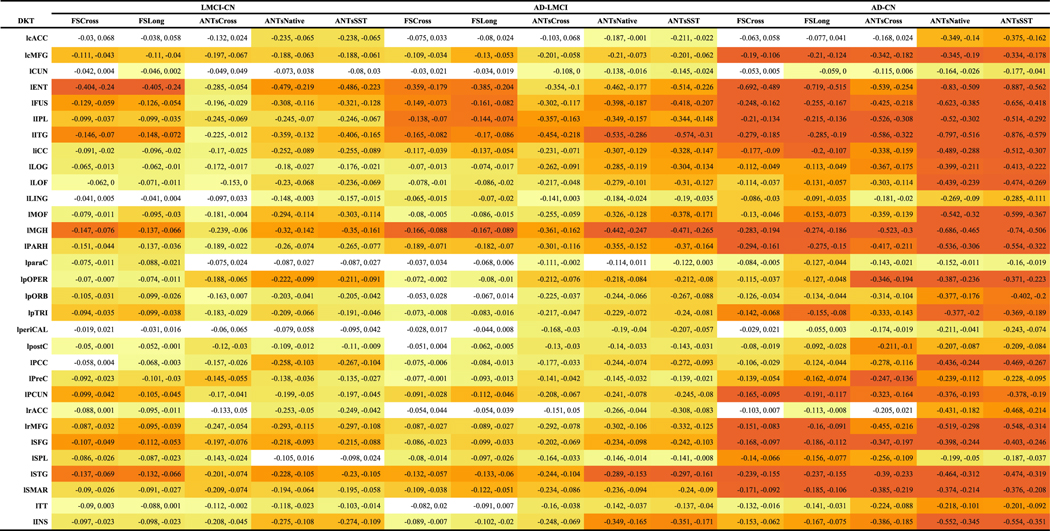
The LME model described in Equation (3) was used to determine region-by-region contrasts for each pairing LMCI—CN, AD—LMCI, and AD—CN using post-hoc Tukey significance testing. It should be noted that no subjects were included that switched diagnostic groups during the acquired study schedule. These findings are provided in Tables 2 and 3. The adjusted p-values were log-scaled for use in specifying the individual color cell for facilitating visual differentiation. Each cell contains the corresponding 95% confidence intervals. Figure 6 provides a side-by-side comparison of the distribution of log-scaled p-values separated into left and right hemispherical components and grouped according to contrast.

Table 2.

95% confidence intervals for the diagnostic contrasts (LMCI–CN, AD–LMCI, AD–CN) of the ADNI-1 data set for each DKT region of the left hemisphere. Each cell is color-coded based on the adjusted log-scaled p-value significance from dark orange (p<1e-10) to yellow (p=0.1). Absence of color denotes nonsignificance

Table 3.

95% confidence intervals for the diagnostic contrasts (LMCI–CN, AD–LMCI, AD–CN) of the ADNI-1 data set for each DKT region of the right hemisphere. Each cell is color-coded based on the adjusted log-scaled p-value significance from dark orange (p<1e-10) to yellow (p=0.1). Absence of color denotes nonsignificance

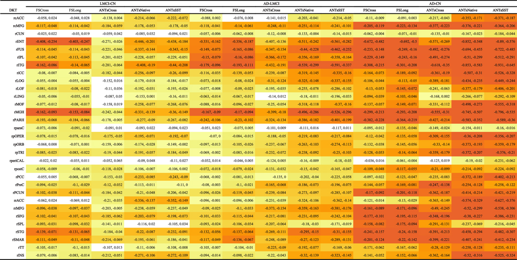
Fig. 6.

Log-scaled p-values summarizing Tables 2 and 3 demonstrating performance differences across cross-sectional and longitudinal pipelines for the three diagnostic contrasts.

Consideration of performance over all three diagnostic pairings illustrates the superiority of the longitudinal ANTs methodologies over their ANTs cross-sectional counterpart. Several regions demonstrating statistically significant non-zero atrophy in ANTs Native and ANTs SST do not mani-fest similar trends in ANTs Cross. Pronounced differences between the ANTs longitudinal versus cross-sectional methodologies can be seen in both the LMCI—CN and AD—CN contrasts. Although ANTs Cross demonstrates discriminative capabilities throughout the cortex and, specifically, in certain AD salient regions, such as the entorhinal and parahippocampal cortices, the contrast is not nearly as strong as the other methods including FS Cross and FS Long thus motivating the use of longitudinal considerations for processing of AD data.

Differentiation between the longitudinal methods is not as obvious although trends certainly exist. In general, for differentiating CN versus LMCI, all methods are comparable except for ANTs Cross. However, for the other two diagnostic contrasts AD—LMCI and AD—CN, the trend is similar to what we found in the evaluation via the variance ratio, viz., the longitudinal ANTs methods tend towards greater contrast means versus ANTs Cross and the two FreeSurfer methods. Looking at specific cortical areas, though, we see that comparable regions(“comparable” in terms of variance ratio)are consistent with previous findings. For example, we noted in the last section that FSLong has a relatively large variance ratio in the entorhinal regions which is consistent with the results seen in Tables 2 and 3.

DISCUSSION

Herein we detailed the ANTs registration-based longitudinal cortical thickness framework which is designed to take advantage of longitudinal data acquisition protocols. This framework has been publicly available as open-source in the ANTs GitHub repository for some time. It has been employed in various neuroimaging studies and this work constitutes a formalized exploration of performance for future reference. It inherits the performance capabilities of the ANTs cross-sectional pipeline providing high reliability for large studies, robust registration and segmentation in human lifespan data, and accurate processing in data (human and animal) which exhibit large shape variation. In addition, the ANTs longitudinal pipeline accounts for the various bias issues that have been associated with processing such data. For example, denoising and N4 bias correction mitigate the effects of noise and intensity artifacts across scanners and visits. The use of the single-subject template provides an unbiased subject-specific reference space and a consistent intermediate space for normalization between the group template and individual time points. Undergirding all normalization components is the well-performing SyN registration algorithm which has demonstrated superior performance for a variety of neuroimaging applications (e.g., [57, 76]) and provides accurate correspondence estimation even in the presence of large anatomical variation. Also, given that the entire pipeline is image-based, conversion issues between surface-and voxel-based representations [77] are non-existent which enhances inclusion of other imaging data and employment of other image-specific tools for multi-modal studies (e.g., tensor-based morphometry, longitudinal cortical labeling using joint label fusion, and the composition of transformations). All ANTs components are built from the Insight Toolkit which leverages the open-source developer community from academic and industrial institutions leading to a robust (e.g., low failure rate) software platform which can run on a variety of platforms.

With respect to these data and AD in general,the ANTs longitudinal cortical thickness pipelines use unbiased diffeomorphic registration to provide robust mapping of individual brains to group template space and, simultaneously, high-resolution sensitivity to subtle longitudinal changes over time. Both advantages are relevant to AD. High baseline atrophy levels in AD lead to the need for robustness to large deformations. Sensitivity to subtle longitudinal change over time is particularly relevant to early or preclinical AD studies due to the relatively reduced atrophy rates and smaller difference from control populations. We demonstrate that our approach leads to competitive or superior estimates of annualized atrophy that are biologically plausible in AD populations and that may, in the future, support the use of T1 neuroimaging to detect treatment effects in clinical trials. Furthermore, in ADNI-1, we report a zero percent failure rate with no subject-specific tuning required.

Over 600 subjects from the well-known longitudinal ADNI-1 data set with diagnoses distributed between cognitively normal, LMCI, and AD were processed through the original ANTs cross-sectional framework [26] and two longitudinal variants. One of the variants, ANTs SST, is similar to the FreeSurfer longitudinal stream in that each time-point image is reoriented to an unbiased single-subject template for subsequent processing. ANTs Native, in contrast, estimates cortical thickness in the native space while also using tissue prior probabilities generated from the SST.

Comparative assessment utilized LME models to determine the between-subject to residual variance ratios over the 62 regions of the brain defined by the DKT parcellation scheme where higher values indicate greater generic statistical salience. In these terms, ANTs SST outperformed all other pipeline variants including both the FreeSurfer longitudinal and cross-sectional streams. Regional disparities between the ANTs SST and Native pipelines point to increases in both between-subject and residual variances which might be due to reorientation to a common space similar to other longitudinal strategies. Further evidence motivating the longitudinal strategies proposed in this work and elsewhere stems from the subsequent exploration of differentiating between diagnostic groups using LMEs with the change in cortical thickness as an outcome variable. Almost across the entire cortex, longitudinal strategies (both ANTs and FreeSurfer) outperformed their cross-sectional counterparts in pairwise differentiation of diagnostic groups although these trends varied based on region and diagnosis. In the context of AD, where certain regions have increased saliency in terms of neuroscientific research, and practical considerations might give more weight to certain diagnostic results over others, further exploration is required to tease out these subtle differences and their implications for future research. Furthermore, future studies, e.g., cross validation and prediction, will provide further understanding of performance characteristics.

One interesting finding was the performance of FS Long in the EC regions where the variance ratios was slightly larger than those of ANTs Long/Native where the credible intervals have significant over-lap. Given the small volume and indistinguishability from surrounding structures, segmentation of the EC can be relatively difficult [78]. This segmentation complexity has led to EC-specific [79] and related [80] strategies for targeted regional [processing. For this work, we wanted to avoid such tuning and simply employ off-the-shelf input parameters and data. Future work will explore refining input template priors in these problematic regions for ANTs-based estimation of cortical thickness.

These findings promote longitudinal analysis considerations and motivates such techniques over cross-sectional methods for longitudinal data despite the increase in computational costs. While we focus on cortical thickness in this work, there are obvious limitations with the ANTs volume-based frame-work. Without a direct reconstruction of the cortical surfaces, many important cortical properties (e.g., surface area, cortical folding, sulcal depth, and gyrification) [81] cannot be generated in a straightforward manner. Additional work will want to examine these features more closely working toward a more comprehensive idea of how structure changes. This will help determine the relative importance of such cortical features and will undoubtedly guide future methodological development. Finally, it should be noted that while the current findings certainly have utility, they are limited to a specific population and the community would benefit from replication and exploration in other populations.

However despite these deficiencies, being inherently voxel-based, the ANTs framework does have advantages not explored in this work but certainly to be utilized in future research. Specifically, the voxel-based input/output processing is conducive to voxel-based analysis strategies (e.g., Eigenanatomy [82]) and straightforward application to non-human research domains. Also, tensor-based morphometric data are directly extracted from the output of the longitudinal processing. And while mesh-based geo-metric measures are unavailable, digital analogs (e.g., surface area from the digitized Crofton formula [46] and surface curvature [83]) provide a convenient data format for integrated data analysis. Finally, given the importance of structural data, such as T1-weighted images, for other types of neuroimaging studies (e.g., resting state fMRI and diffusion tensor imaging), the longitudinal processing stream provides convenient output for facilitating these other types of analyses.

The ANTs longitudinal pipeline provides several additional features that may be worth investigation in future studies. The segmentation approach provides tissue probability maps that may be used in identifying abnormalities of WM or in voxel-wise studies of GM density. The longitudinal formulation of the pipeline is also likely to improve the variance ratio for other transformation based measurements such as the log-jacobian, often employed in tensor-based morphometry [84]. Local folding and other curvature-based metrics are available, as well, through ANTsR [85]. These quantification tools, individually or jointly, may provide insight into aging and neurodegeneration and will be the subject of future evaluation efforts.

The longitudinal thickness framework is available in script form within the ANTs software library along with the requisite processing components (Supplementary Material). All generated data used for input, such as the ADNI template and tissue priors, are available upon request. As previously mentioned, we also make available the csv files containing the regional thickness values for all three pipelines.

REFERENCES

- [1].Du A-T, Schuff N, Kramer JH, Rosen HJ, Gorno-Tempini ML, Rankin K, Miller BL, Weiner MW (2007) Different regional patterns of cortical thinning in Alzheimer’s disease and frontotemporal dementia. Brain 130, 1159–1166. [DOI] [PMC free article] [PubMed] [Google Scholar]
- [2].Dickerson BC, Bakkour A, Salat DH, Feczko E, Pacheco J, Greve DN, Grodstein F, Wright CI, Blacker D, Rosas HD, Sperling RA, Atri A, Growdon JH, Hyman BT, Morris JC, Fischl B, Buckner RL (2009) The cortical signature of Alzheimer’s disease: Regionally specific cortical thinning relates to symptom severity in very mild to mild AD dementia and is detectable in asymptomatic amyloid-positive individuals. Cereb Cortex 19, 497–510. [DOI] [PMC free article] [PubMed] [Google Scholar]
- [3].MacDonald D, Kabani N, Avis D, Evans AC (2000) Auto-mated 3-D extraction of inner and outer surfaces of cerebral cortex from MRI. Neuroimage 12, 340–356. [DOI] [PubMed] [Google Scholar]
- [4].Magnotta VA, Andreasen NC, Schultz SK, Harris G, Cizadlo T, Heckel D, Nopoulos P, Flaum M (1999) Quantitative in vivo measurement of gyrification in the human brain: Changes associated with aging. Cereb Cortex 9, 151–160. [DOI] [PubMed] [Google Scholar]
- [5].Kim JS, Singh V, Lee JK, Lerch J, Ad-Dab’bagh Y, Mac-Donald D, Lee JM, Kim SI, Evans AC (2005) Automated 3-D extraction and evaluation of the inner and outer cortical surfaces using a Laplacian map and partial volume effect classification. Neuroimage 27, 210–221. [DOI] [PubMed] [Google Scholar]
- [6].Zeng X, Staib LH, Schultz RT, Duncan JS (1999) Segmentation and measurement of the cortex from 3-D MR images using coupled-surfaces propagation.IEEE Trans Med Imaging 18, 927–937. [DOI] [PubMed] [Google Scholar]
- [7].Jones SE, Buchbinder BR, Aharon I (2000) Three-dimensional mapping of cortical thickness using Laplace’s equation. Hum Brain Mapp 11, 12–32. [DOI] [PMC free article] [PubMed] [Google Scholar]
- [8].Das SR, Avants BB, Grossman M, Gee JC (2009) Registration based cortical thickness measurement. Neuroimage 45, 867–879. [DOI] [PMC free article] [PubMed] [Google Scholar]
- [9].Vachet C, Hazlett HC, Niethammer M, Oguz I, Cates J, Whitaker R, Piven J, Styner M (2011) Group-wise automatic mesh-based analysis of cortical thickness. In SPIE medical imaging: Image processing, Benoit M. Dawant DRH, ed. [Google Scholar]
- [10].Kraemer HC, Yesavage JA, Taylor JL, Kupfer D (2000) How can we learn about developmental processes from cross sectional studies, or can we? Am J Psychiatry 157, 163–171. [DOI] [PubMed] [Google Scholar]
- [11].Weiner MW, Veitch DP, Aisen PS, Beckett LA, Cairns NJ, Green RC, Harvey D, Jack CR, Jagust W, Liu E, Morris JC, Petersen RC, Saykin AJ, Schmidt ME, Shaw L, Siuciak JA, Soares H, Toga AW, Trojanowski JQ, Alzheimer’s Disease Neuroimaging Initiative (2012) The Alzheimer’s disease neuroimaging initiative: A review of papers published since its inception. Alzheimers Dement 8, S1–68. [DOI] [PMC free article] [PubMed] [Google Scholar]
- [12].Reuter M, Schmansky NJ, Rosas HD, Fischl B (2012) Within-subject template estimation for unbiased longitudinal image analysis. Neuroimage 61, 1402–1418. [DOI] [PMC free article] [PubMed] [Google Scholar]
- [13].Smith SM, Zhang Y, Jenkinson M, Chen J, Matthews PM, Federico A, De Stefano N (2002) Accurate, robust, and automated longitudinal and cross-sectional brain change analysis. Neuroimage 17, 479–489. [DOI] [PubMed] [Google Scholar]
- [14].Yushkevich PA, Avants BB, Das SR, Pluta J, Altinay M, Craige C, Alzheimer’s Disease Neuroimaging Initiative (2010) Bias in estimation of hippocampal atrophy using deformation-based morphometry arises from asymmetric global normalization: An illustration in ADNI 3 T MRI data. Neuroimage 50, 434–445. [DOI] [PMC free article] [PubMed] [Google Scholar]
- [15].Thompson WK, Holland D, Alzheimer’s Disease Neuroimaging Initiative (2011) Bias in tensor based morphom-etry stat-ROI measures may result in unrealistic power estimates. Neuroimage 57, 1–4. [DOI] [PMC free article] [PubMed] [Google Scholar]
- [16].Avants B, Cook PA, McMillan C, Grossman M, Tustison NJ, Zheng Y, Gee JC (2010) Sparse unbiased analysis of anatomical variance in longitudinal imaging. Med Image Comput Comput Assist Interv 13, 324–331. [DOI] [PMC free article] [PubMed] [Google Scholar]
- [17].Fox NC, Ridgway GR, Schott JM (2011) Algorithms, atrophy and Alzheimer’s disease: Cautionary tales for clinical trials. Neuroimage 57, 15–18. 1022 [DOI] [PubMed] [Google Scholar]
- [18].Hua X, Hibar DP, Ching CRK, Boyle CP, Rajagopalan P, Gutman BA, Leow AD, Toga AW, Jack CR Jr, Har-vey D, Weiner MW, Thompson PM, Alzheimer’s Disease Neuroimaging Initiative (2013) Unbiased tensor-based mor-phometry: Improved robustness and sample size estimates for Alzheimer’s disease clinical trials. Neuroimage 66, 1028 648–661. [DOI] [PMC free article] [PubMed] [Google Scholar]
- [19].Reuter M, Fischl B (2011) Avoiding asymmetry-induced 1030 bias in longitudinal image processing. Neuroimage 57, 19–21. [DOI] [PMC free article] [PubMed] [Google Scholar]
- [20].Bernal-Rusiel JL, Greve DN, Reuter M, Fischl B, Sabuncu MR, Alzheimer’s Disease Neuroimaging Initiative (2013) Statistical analysis of longitudinal neuroimage data with linear mixed effects models. Neuroimage 66, 249–260. [DOI] [PMC free article] [PubMed] [Google Scholar]
- [21].Wierenga LM, Langen M, Oranje B, Durston S (2014) Unique developmental trajectories of cortical thickness and surface area. Neuroimage 87, 120–126. [DOI] [PubMed] [Google Scholar]
- [22].Landin-Romero R, Kumfor F, Leyton CE, Irish M, Hodges JR, Piguet O (2017) Disease-specific patterns of cortical and subcortical degeneration in a longitudinal study of Alzheimer’s disease and behavioural-variant frontotempo-ral dementia. Neuroimage 151, 72–80. [DOI] [PubMed] [Google Scholar]
- [23].Nourbakhsh B, Azevedo C, Nunan-Saah J, Maghzi A-H, Spain R, Pelletier D, Waubant E (2016) Longitudinal associations between brain structural changes and fatigue in early MS. Mult Scler Relat Disord 5, 29–33. [DOI] [PubMed] [Google Scholar]
- [24].Li G, Nie J, Wang L, Shi F, Gilmore JH, Lin W, Shen D (2014) Measuring the dynamic longitudinal cortex development in infants by reconstruction of temporally consistent cortical surfaces. Neuroimage 90, 266–279. [DOI] [PMC free article] [PubMed] [Google Scholar]
- [25].Nakamura K, Fox R, Fisher E (2011) CLADA: Cortical longitudinal atrophy detection algorithm. Neuroimage 54, 278–289. [DOI] [PMC free article] [PubMed] [Google Scholar]
- [26].Tustison NJ, Cook PA, Klein A, Song G, Das SR, Duda JT, Kandel BM, Strien N van, Stone JR, Gee JC, Avants BB (2014) Large-scale evaluation of ANTs and FreeSurfer cortical thickness measurements. Neuroimage 99, 166–179. [DOI] [PubMed] [Google Scholar]
- [27].Fujishima M, Maikusa N, Nakamura K, Nakatsuka M, Matsuda H, Meguro K (2014) Mild cognitive impairment, poor episodic memory, and late-life depression are associated with cerebral cortical thinning and increased white matter hyperintensities. Front Aging Neurosci 6, 306. [DOI] [PMC free article] [PubMed] [Google Scholar]
- [28].Das SR, Mancuso L, Olson IR, Arnold SE, Wolk DA (2016) Short-term memory depends on dissociable medial temporal lobe regions in amnestic mild cognitive impairment. Cereb Cortex 26, 2006–2017. [DOI] [PMC free article] [PubMed] [Google Scholar]
- [29].Olm CA, Kandel BM, Avants BB, Detre JA, Gee JC, Grossman M, McMillan CT (2016) Arterial spin labeling perfusion predicts longitudinal decline in semantic variant primary progressive aphasia. J Neurol 263, 1927–1938. [DOI] [PMC free article] [PubMed] [Google Scholar]
- [30].Pagani M, Damiano M, Galbusera A, Tsaftaris SA, Gozzi A (2016) Semi-automated registration-based anatomical labelling, voxel based morphometry and cortical thickness mapping of the mouse brain. J Neurosci Methods 267, 62–73. [DOI] [PubMed] [Google Scholar]
- [31].Majka P, Chaplin TA, Yu H-H, Tolpygo A, Mitra PP, Wojcik ´ DK, Rosa MGP (2016) Towards a comprehensive atlas of cortical connections in a primate brain: Mapping tracer injection studies of the common marmoset into a reference digital template. J Comp Neurol 524, 2161–2181. [DOI] [PMC free article] [PubMed] [Google Scholar]
- [32].Mugler JP 3rd, Brookeman JR (1990) Three-dimensional magnetization-prepared rapid gradient-echo imaging (3D MP RAGE). Magn Reson Med 15, 152–157. [DOI] [PubMed] [Google Scholar]
- [33].Jack CR Jr, Bernstein MA, Fox NC, Thompson P, Alexander G, Harvey D, Borowski B, Britson PJ, L Whitwell J, Ward C, Dale AM, Felmlee JP, Gunter JL, Hill DLG, Killiany R, Schuff N, Fox-Bosetti S, Lin C, Studholme C, DeCarli CS, Krueger G, Ward HA, Metzger GJ, Scott KT, Mallozzi R, Blezek D, Levy J, Debbins JP, Fleisher AS, Albert M, Green R, Bartzokis G, Glover G, Mugler J, Weiner MW (2008) The Alzheimer’s Disease Neuroimaging Initiative (ADNI): MRI methods. J Magn Reson Imaging 27, 685–691. [DOI] [PMC free article] [PubMed] [Google Scholar]
- [34].Tustison NJ, Avants BB, Cook PA, Zheng Y, Egan A, Yushkevich PA, Gee JC (2010) N4ITK: Improved N3 bias correction. IEEE Trans Med Imaging 29, 1310–1320. [DOI] [PMC free article] [PubMed] [Google Scholar]
- [35].Avants BB, Klein A, Tustison NJ, Woo J, Gee JC (2010) Evaluation of an open-access, automated brain extraction method on multi-site multi-disorder data. 16th annual meeting for the Organization of Human Brain Mapping. [Google Scholar]
- [36].Avants BB, Tustison NJ, Wu J, Cook PA, Gee JC (2011) An open source multivariate framework for n-tissue segmentation with evaluation on public data. Neuroinformatics 9, 381–400 [DOI] [PMC free article] [PubMed] [Google Scholar]
- [37].Wang H, Suh JW, Das SR, Pluta JB, Craige C, Yushkevich PA (2013) Multi-atlas segmentation with joint label fusion. IEEE Trans Pattern Anal Mach Intell 35, 611–623. [DOI] [PMC free article] [PubMed] [Google Scholar]
- [38].Klein A, Tourville J (2012) 101 labeled brain images and a consistent human cortical labeling protocol. Front Neurosci 6, 171. [DOI] [PMC free article] [PubMed] [Google Scholar]
- [39].Tustison NJ, Herrera JM (2016) Two Luis Miguel fans walk into a bar in Nagoya —>(yada, yada, yada) —>an ITKimplementation of a popular patch-based denoising filter. Insight J, http://hdl.handle.net/10380/3564 [Google Scholar]
- [40].Manjon JV, Coupe P, Mart ´ ´ı-Bonmat´ı L, Collins DL, Robles M (2010) Adaptive non-local means denoising of MR images with spatially varying noise levels. J Magn Reson Imaging 31, 192–203. [DOI] [PubMed] [Google Scholar]
- [41].Avants BB, Tustison NJ, Song G, Cook PA, Klein A, Gee JC (2011) A reproducible evaluation of ANTs similarity metric performance in brain image registration. Neuroimage 54, 2033–2044. [DOI] [PMC free article] [PubMed] [Google Scholar]
- [42].Avants BB, Tustison NJ, Stauffer M, Song G, Wu B, Gee JC (2014) The Insight ToolKit image registration framework. Front Neuroinform 8, 44. [DOI] [PMC free article] [PubMed] [Google Scholar]
- [43].Landman BA, Huang AJ, Gifford A, Vikram DS, Lim IAL, Farrell JAD, Bogovic JA, Hua J, Chen M, Jarso S, Smith SA, Joel S, Mori S, Pekar JJ, Barker PB, Prince JL, Zijl PCM van (2011) Multi-parametric neuroimaging reproducibility: A 3-T resource study. Neuroimage 54, 2854–2866. [DOI] [PMC free article] [PubMed] [Google Scholar]
- [44].Nooner KB, Colcombe SJ, Tobe RH, Mennes M, Benedict MM, Moreno AL, Panek LJ, Brown S, Zavitz ST, Li Q, Sikka S, Gutman D, Bangaru S, Schlachter RT, Kamiel SM, Anwar AR, Hinz CM, Kaplan MS, Rachlin AB, Adelsberg S, Cheung B, Khanuja R, Yan C, Craddock CC, Calhoun V, Courtney W, King M, Wood D, Cox CL, Kelly AMC, Di Martino A, Petkova E, Reiss PT, Duan N, Thomsen D, Biswal B, Coffey B, Hoptman MJ, Javitt DC, Pomara N, Sidtis JJ, Koplewicz HS, Castellanos FX, Leventhal BL, Milham MP (2012) The NKI-rockland sample: A model for accelerating the pace of discovery science in psychiatry. Front Neurosci 6, 152. [DOI] [PMC free article] [PubMed] [Google Scholar]
- [45].Breiman L (2001) Random forests. In Machine learning, pp. 5–32. [Google Scholar]
- [46].Lehmann G, Legland D (2012) Efficient N-dimensional surface estimation using Crofton formula and run-length encoding. Insight J, http://hdl.handle.net/10380/3342. [Google Scholar]
- [47].Hasan KM, Mwangi B, Cao B, Keser Z, Tustison NJ, Kochunov P, Frye RE, Savatic M, Soares J (2016) Entorhinal cortex thickness across the human lifespan. J Neuroimaging 26, 278–82. [DOI] [PMC free article] [PubMed] [Google Scholar]
- [48].Price AR, Bonner MF, Peelle JE, Grossman M (2015) Converging evidence for the neuroanatomic basis of combinatorial semantics in the angular gyrus. J Neurosci 35, 3276–3284. [DOI] [PMC free article] [PubMed] [Google Scholar]
- [49].Wisse LEM, Butala N, Das SR, Davatzikos C, Dickerson BC, Vaishnavi SN, Yushkevich PA, Wolk DA, Alzheimer’s Disease Neuroimaging Initiative (2015) Suspected non-AD pathology in mild cognitive impairment. Neurobiol Aging 36, 3152–3162. [DOI] [PMC free article] [PubMed] [Google Scholar]
- [50].Betancourt LM, Avants B, Farah MJ, Brodsky NL, Wu J, Ashtari M, Hurt H (2015) Effect of socioeconomic status (ses) disparity on neural development in female AfricanAmerican infants at age 1 month. Dev Sci 19, 947–956. [DOI] [PubMed] [Google Scholar]
- [51].Avants BB, Yushkevich P, Pluta J, Minkoff D, Korczykowski M, Detre J, Gee JC (2010) The optimal template effect in hippocampus studies of diseased populations. Neuroimage 49, 2457–2466. [DOI] [PMC free article] [PubMed] [Google Scholar]
- [52].Buades A (2005) A non-local algorithm for image denoising. Comp Vis Pattern Recognit 2, 60–65. [Google Scholar]
- [53].Gudbjartsson H, Patz S (1995) The Rician distribution of noisy MRI data. Magn Reson Med 34, 910–914. [DOI] [PMC free article] [PubMed] [Google Scholar]
- [54].Coupe P, Manjon JV, Fonov V, Pruessner J, Robles M, ´ Collins DL (2011) Patch-based segmentation using expert priors: Application to hippocampus and ventricle segmentation. Neuroimage 54, 940–954. [DOI] [PubMed] [Google Scholar]
- [55].Cousijn J, Wiers RW, Ridderinkhof KR, Brink W van den, Veltman DJ, Goudriaan AE (2012) Grey matter alterations associated with cannabis use: Results of a VBM study in heavy cannabis users and healthy controls. Neuroimage 59, 3845–3851. [DOI] [PubMed] [Google Scholar]
- [56].Abutalebi J, Canini M, Della Rosa PA, Sheung LP, Green DW, Weekes BS (2014) Bilingualism protects anterior temporal lobe integrity in aging. Neurobiol Aging 35, 2126–2133. [DOI] [PubMed] [Google Scholar]
- [57].Tustison NJ, Shrinidhi KL, Wintermark M, Durst CR, Kandel BM, Gee JC, Grossman MC, Avants BB (2015) Optimal symmetric multimodal templates and concatenated random forests for supervised brain tumor segmentation (simplified) with ANTsR. Neuroinformatics 13, 209–225. [DOI] [PubMed] [Google Scholar]
- [58].Rosas HD, Liu AK, Hersch S, Glessner M, Ferrante RJ, Salat DH, Kouwe A van der, Jenkins BG, Dale AM, Fischl B (2002) Regional and progressive thinning of the cortical ribbon in Huntington’s disease. Neurology 58, 695–701. [DOI] [PubMed] [Google Scholar]
- [59].Kuperberg GR, Broome MR, McGuire PK, David AS, Eddy M, Ozawa F, Goff D, West WC, Williams SCR, Kouwe AJW van der, Salat DH, Dale AM, Fischl B (2003) Regionally localized thinning of the cerebral cortex in schizophrenia. Arch Gen Psychiatry 60, 878–888. [DOI] [PubMed] [Google Scholar]
- [60].Jovicich J, Marizzoni M, Sala-Llonch R, Bosch B, Bartres-´ Faz D, Arnold J, Benninghoff J, Wiltfang J, Roccatagliata L, Nobili F, Hensch T, Trankner A, Schonknecht P, Leroy M, Lopes R, Bordet R, Chanoine V, Ranjeva J-P, Didic M, Gros-Dagnac H, Payoux P, Zoccatelli G, Alessandrini F, Beltramello A, Bargallo N, Blin O, Frisoni GB, The PharmaCog Consortium (2013) Brain morphometry reproducibility in multi-center 3T MRI studies: A comparison of crosssectional and longitudinal segmentations. Neuroimage 83, 472–484. [DOI] [PubMed] [Google Scholar]
- [61].Klein A, Ghosh SS, Bao FS, Giard J, Hame Y, Stavsky E, Lee N, Rossa B, Reuter M, Chaibub Neto E, Keshavan A (2017) Mindboggling morphometry of human brains. PLoS Comput Biol 13, e1005350. [DOI] [PMC free article] [PubMed] [Google Scholar]
- [62].Li G, Nie J, Wu G, Wang Y, Shen D, Alzheimer’s Disease Neuroimaging Initiative (2012) Consistent reconstruction of cortical surfaces from longitudinal brain MR images. Neuroimage 59, 3805–3820. [DOI] [PMC free article] [PubMed] [Google Scholar]
- [63].Verbeke G, Molenberghs G (2009) Linear mixed models for longitudinal data, Springer Science & Business Media. [Google Scholar]
- [64].Fitzmaurice GM, Laird NM, Ware JH (2012) Applied longitudinal analysis, John Wiley & Sons. [Google Scholar]
- [65].Gelman A (2006) Prior distributions for variance parameters in hierarchical models. Bayesian Anal 1, 515–533. [Google Scholar]
- [66].Carpenter B, Gelman A, Hoffman M, Lee D, Goodrich B, Betancourt M, Brubaker MA, Guo J, Li P, Riddell A (2016) Stan: A probabilistic programming language. J Stat Softw 76, doi: 10.18637/jss.v076.i01 [DOI] [PMC free article] [PubMed] [Google Scholar]
- [67].Seber GA, Lee AJ (2012) Linear regression analysis, John Wiley & Sons. [Google Scholar]
- [68].Fuller WA (2009) Measurement error models, John Wiley & Sons. [Google Scholar]
- [69].Carroll RJ, Ruppert D, Stefanski LA, Crainiceanu CM (2006) Measurement error in nonlinear models: A modern perspective, CRC press. [Google Scholar]
- [70].Yassa MA (2014) Ground zero in alzheimer’s disease. Nat Neurosci 17, 146–147. [DOI] [PubMed] [Google Scholar]
- [71].Schmitz TW, Nathan Spreng R, Alzheimer’s Disease Neuroimaging Initiative (2016) Basal forebrain degeneration precedes and predicts the cortical spread of Alzheimer’s pathology. Nat Commun 7, 13249. [DOI] [PMC free article] [PubMed] [Google Scholar]
- [72].Andrews KA, Frost C, Modat M, Cardoso MJ, AIBL, Rowe CC, Villemagne V, Fox NC, Ourselin S, Schott JM (2016) Acceleration of hippocampal atrophy rates in asymptomatic amyloidosis. Neurobiol Aging 39, 99–107. [DOI] [PubMed] [Google Scholar]
- [73].Crutch SJ, Schott JM, Rabinovici GD, Murray M, Snowden JS, Flier WM van der, Dickerson BC, Vandenberghe R, Ahmed S, Bak TH, Boeve BF, Butler C, Cappa SF, Ceccaldi M, Souza LC de, Dubois B, Felician O, Galasko D, Graff-Radford J, Graff-Radford NR, Hof PR, KrolakSalmon P, Lehmann M, Magnin E, Mendez MF, Nestor PJ, Onyike CU, Pelak VS, Pijnenburg Y, Primativo S, Rossor MN, Ryan NS, Scheltens P, Shakespeare TJ, Suarez ´ Gonzalez A, Tang-Wai DF, Yong KXX, Carrillo M, Fox NC, Alzheimer’s Association ISTAART Atypical Alzheimer’s Disease and Associated Syndromes Professional Interest Area (2017) Consensus classification of posterior cortical atrophy. Alzheimers Dement 13, 870–884. [DOI] [PMC free article] [PubMed] [Google Scholar]
- [74].Falahati F, Ferreira D, Muehlboeck J-S, Eriksdotter M, Simmons A, Wahlund L-O, Westman E (2017) Monitoring disease progression in mild cognitive impairment: Associations between atrophy patterns, cognition, APOE and amyloid. Neuroimage Clin 16, 418–428. [DOI] [PMC free article] [PubMed] [Google Scholar]
- [75].Bates D, Machler M, Bolker B, Walker S (2015) Fitting linear mixed-effects models using lme4. J Stat Softw, 67, 1–48. [Google Scholar]
- [76].Klein A, Andersson J, Ardekani BA, Ashburner J, Avants B, Chiang M-C, Christensen GE, Collins DL, Gee J, Hellier P, Song JH, Jenkinson M, Lepage C, Rueckert D, Thompson P, Vercauteren T, Woods RP, Mann JJ, Parsey RV (2009) Evaluation of 14 nonlinear deformation algorithms applied to human brain MRI registration. Neuroimage 46, 786–802. [DOI] [PMC free article] [PubMed] [Google Scholar]
- [77].Klein A, Ghosh SS, Avants B, Yeo BTT, Fischl B, Ardekani B, Gee JC, Mann JJ, Parsey RV (2010) Evaluation of volume-based and surface-based brain image registration methods. Neuroimage 51, 214–220 [DOI] [PMC free article] [PubMed] [Google Scholar]
- [78].Price CC, Wood MF, Leonard CM, Towler S, Ward J, Montijo H, Kellison I, Bowers D, Monk T, Newcomer JC, Schmalfuss I (2010) Entorhinal cortex volume in older adults: Reliability and validity considerations for three published measurement protocols. J Int Neuropsychol Soc 16, 846–855. [DOI] [PMC free article] [PubMed] [Google Scholar]
- [79].Fischl B, Stevens AA, Rajendran N, Yeo BTT, Greve DN, Van Leemput K, Polimeni JR, Kakunoori S, Buckner RL, Pacheco J, Salat DH, Melcher J, Frosch MP, Hyman BT, Grant PE, Rosen BR, Kouwe AJW van der, Wiggins GC, Wald LL, Augustinack JC (2009) Predicting the location of entorhinal cortex from MRI. Neuroimage 47, 8–17. [DOI] [PMC free article] [PubMed] [Google Scholar]
- [80].Augustinack JC, Huber KE, Stevens AA, Roy M, Frosch MP, Kouwe AJW van der, Wald LL, Van Leemput K, McKee AC, Fischl B, Alzheimer’s Disease Neuroimaging Initiative (2013) Predicting the location of human perirhinal cortex, Brodmann’s area 35, from MRI. Neuroimage 64, 32–42. [DOI] [PMC free article] [PubMed] [Google Scholar]
- [81].Shimony JS, Smyser CD, Wideman G, Alexopoulos D, Hill J, Harwell J, Dierker D, Van Essen DC, Inder TE, Neil JJ (2016) Comparison of cortical folding measures for evaluation of developing human brain. Neuroimage 125, 780–790. [DOI] [PMC free article] [PubMed] [Google Scholar]
- [82].Kandel BM, Wang DJJ, Gee JC, Avants BB (2015) Eigenanatomy: Sparse dimensionality reduction for multi-modal medical image analysis. Methods 73, 43–53. [DOI] [PMC free article] [PubMed] [Google Scholar]
- [83].Avants B, Gee J (2003) The shape operator for differential analysis of images. Inf Process Med Imaging 18, 101–13. [DOI] [PubMed] [Google Scholar]
- [84].Vemuri P, Senjem ML, Gunter JL, Lundt ES, Tosakulwong N, Weigand SD, Borowski BJ, Bernstein MA, Zuk SM, Lowe VJ, Knopman DS, Petersen RC, Fox NC, Thompson PM, Weiner MW, Jack CR Jr, Alzheimer’s Disease Neuroimaging Initiative (2015) Accelerated vs. unaccelerated serial MRI based TBM-SYN measurements for clinical trials in Alzheimer’s disease. Neuroimage 113, 61–69. [DOI] [PMC free article] [PubMed] [Google Scholar]
- [85].Muschelli J, Gherman A, Fortin J-P, Avants B, Whitcher B, Clayden JD, Caffo BS, Crainiceanu CM (2019) Neu-roconductor: An r platform for medical imaging analysis. Biostatistics 20, 218–239 [DOI] [PMC free article] [PubMed] [Google Scholar]
Associated Data
This section collects any data citations, data availability statements, or supplementary materials included in this article.