A Unique Color-Coded Visualization System with Multimodal Information Fusion and Deep Learning in a Longitudinal Study of Alzheimer’s Disease

Abstract

Purpose:

Automated diagnosis and prognosis of Alzheimer’s Disease remain a challenging problem that machine learning (ML) techniques have attempted to resolve in the last decade. This study introduces a first-of-its-kind color-coded visualization mechanism driven by an integrated ML model to predict disease trajectory in a 2-year longitudinal study. The main aim of this study is to help capture visually in 2D and 3D renderings the diagnosis and prognosis of AD, therefore augmenting our understanding of the processes of multiclass classification and regression analysis.

Method:

The proposed method, Machine Learning for Visualizing AD (ML4VisAD), is designed to predict disease progression through a visual output. This newly developed model takes baseline measurements as input to generate a color-coded visual image that reflects disease progression at different time points. The architecture of the network relies on convolutional neural networks. With 1,123 subjects selected from the ADNI QT-PAD dataset, we use a 10-fold cross-validation process to evaluate the method. Multimodal inputs^* include neuroimaging data (MRI, PET), neuropsychological test scores (excluding MMSE, CDR-SB, and ADAS to avoid bias), cerebrospinal fluid (CSF) biomarkers with measures of amyloid beta (ABETA), phosphorylated tau protein (PTAU), total tau protein (TAU), and risk factors that include age, gender, years of education, and ApoE4 gene.

Findings/Results:

Based on subjective scores reached by three raters, the results showed an accuracy of 0.82±0.03 for a 3-way classification and 0.68±0.05 for a 5-way classification. The visual renderings were generated in 0.08 msec for a 23×23 output image and in 0.17 msec for a 45×45 output image. Through visualization, this study (1) demonstrates that the ML visual output augments the prospects for a more accurate diagnosis and (2) highlights why multiclass classification and regression analysis are incredibly challenging. An online survey was conducted to gauge this visualization platform’s merits and obtain valuable feedback from users. All implementation codes are shared online on GitHub.

Conclusion:

This approach makes it possible to visualize the many nuances that lead to a specific classification or prediction in the disease trajectory, all in context to multimodal measurements taken at baseline. This ML model can serve as a multiclass classification and prediction model while reinforcing the diagnosis and prognosis capabilities by including a visualization platform.

1. Introduction

The challenges of understanding AD and its prodromal stages are associated with the meaningful interpretation of the interplay between the different biomarkers for diagnosis, multiclass classification, and regression analysis, especially as it relates to the pathogenesis of the disease [1, 2, 3, 4, 5] and its early detection [6, 7]. There is also wide-ranging deliberation on the nature of cognitive reserve [8, 9], potentially biasing the neuropsychological examinations and, ultimately, the diagnosis. Additionally, there is the issue of chronology in the manifestation of amyloid-beta plaques and tau tangles [10, 11, 12] and their synergistic effects on AD pathology. We also need to consider APOE genotypes [13, 14, 15] for their association with a cognitive reserve and cortical thinning, as well as with its potential link to both amyloid-beta, tau aggregation, and the cerebrospinal fluid (CSF) biomarkers [16, 17]. The central aim of all these studies is to identify the earliest manifestations of AD to take preventive measures and provide early treatment/therapeutic interventions [18, 19].

Implementing machine learning is an effective way to approach the complex challenge of multimodal data [20, 21, 22]. However, ML models are not always easily interpretable. Visualization of the ML results can enhance our understanding of the inner workings of the algorithmic process in context to what it has learned from the baseline measurements. The assertation here is that visualization will enhance the means to assess the importance of features and the interpretability of results [23–25].

Using the “QT-PAD Project Data” from the Alzheimer’s Disease Modelling Challenge [http://www.pi4cs.org/qt-pad-challenge], the proposed machine learning, named Machine Learning for Visualizing AD (ML4VisAD), construct aims to produce a color-coded visualization scheme with a unique tensorization method to yield images that express disease state and progression through the different time points in a longitudinal study. Although the goals of high accuracy in multiclass classification and prediction of disease trajectory using only baseline features is essential, the information provided visually by the ML4VisAD model brings forth subtle nuances of the machine learning decision-making process, which is especially crucial when dealing with converter cases. Ultimately, the proposed visualization method exemplifies the challenges faced in multimodal and multiclass classification and the decision-making process. Visualization may also shed some light on the “black box” problem associated with machine learning. Moreover, ML4VisAD will also augment the deliberation process through a visual opportunity to reassess ambiguous cases, like the converter cases, to determine whether a misclassification happened or that the ML visual outcome is the one projecting a correct classification, although different from the target image. In such a case, clinicians could deliberate on the visual output in context to the available measurements.

Along this line of research, the studies reported in [20, 21] suggest that most machine/deep learning methods rely more often on data-related issues, proposed methodologies, and the different clinical aspects under study but ignore visualization. Similarly, most studies emphasize the relevant clinical features and the computational methods, which are more likely to produce high classification and prediction results [20, 26, 27]. Machine learning can also help develop medical imaging methods that address the challenging task of segmentation and noise removal [28, 29, 30]. Also, in [31], efforts are made at data reduction and using different data visualization techniques to embed complex information in 2-D images to reflect gene expression and clinical data for diagnosis.

Several other studies focused their classification and prediction algorithms on visualizing data in a dimensionally reduced decisional space. The dimensionality reduction methods typically involve the use of principal component analysis (PCA), locally linear embedding (LLE), latent profile analysis (LPA), 3D scattering transforms, and the concept of histones [32–45]. Traditionally, standard methods used to aid in the visualization and diagnosis of AD typically involve heat maps, brain connectivity maps, and specific AD signatures, such as Standard Uptake Value Ratios (SUVRs) of disease-prone brain regions [46–53]. All methods that address the challenge of high-dimensional data also use visualization methods that produce optimal decisional spaces helpful to the classification process but not necessarily geared towards facilitating a visual interpretation of a diagnosis and prognosis of the disease which ML4VisAD seeks to address.

The manuscript’s structure is as follows: Section 2 provides the details of the data used in this study and the methods implemented, including the color-coding mechanism, the machine learning architecture, and its computational capability. Section 3 reports the results of varying disease states and disease progression cases. Section 4 provides a discussion reflecting on the different findings and merits of the proposed ML4VisAD model. Finally, Section 5 concludes with a retrospective on the contributions made, highlighting the complexity faced when using machine learning for multiclass classification and prediction in AD.

2. Methods

2.1. Study design

Clinical data used in the preparation of this study is from the Alzheimer’s Disease Neuroimaging Initiative (ADNI) database (adni.loni.usc.edu). Only subjects that have a baseline (T0) scan (in at least one modality) and showed up for follow-up visits at T6 (6th month), T12 (12th month), and T24 (24th month) have been considered in this study, leading to a total of 1123 subjects as shown in Table 1. ADNI categorizes these subjects into the three classes of CN, MCI, and AD at baseline and for each referral session.

Table 1:

Study population and subgroups

Categories based on diagnosis					Categories based on conversion
	Number of samples #			Total				#	Description
	CN	AD	MCI			CN		329	Stable Normal
Baseline	331	163	629	1123		Others		8	Others (e.g. MCI to CN)
6th month	331	195	597	1123		Impaired	AD	163	Stable Dementia
12th month	332	243	548	1123
							MCI	442	Stable MCI
24th month	334	342	447	1123
							MCIc	181	MCI converter to AD
								786	Total Impaired
								1123	Total

The input features used for each modality and the number of observations made at the different time points are obtained from the “QT-PAD Project Data” AD Modelling Challenge [http://www.pi4cs.org/qt-pad-challenge] as given in Table 2. Hence, inputs to the ML model contain features from the baseline, including MRI and PET sequences, demographic information, and specific cognitive measurements. Automatically generated outputs of the ML network are images containing colorful strips expressing disease progression at different time points. It is important to emphasize that in designing this color-coded visualization scheme, and to avoid any bias, we exclude the Mini-Mental State Examination (MMSE) and the Clinical Dementia Rating Sum of Boxes (CDR-SB) scores from the input feature space in the training and testing phases since both are used for the labeling of subjects. Furthermore, we also remove from consideration the Alzheimer’s Disease Assessment Scores (ADAS11, ADAS13) as they correlate well with MMSE and CDR-SB. Each feature $f$ of the input feature vector, e.g. FDG, is normalized by mean normalization over all its non-missing values (set $F$) i.e. $f\_normalized=(f-mean(F\left)\right)/\left(max\right(F)-min(F\left)\right)$.

Table 2-.

ADNI (QT-pad challenge) dataset with the features extracted from each modality/source at baseline

Number of subjects: 1123
Modality	Feature	Minimum Value	Average Value	Maximum Value	Number of missed values at baseline
MRI	Ventricular volume	5650.0	39420.220	145115.0	39
	Hippocampus volume	3091.0	6798.67	10769.0	158
	Whole Brain volume	738813.0	1022118.21	1443990.50	18
	Entorhinal Cortical thickness	1426.0	3507.23	5896.0	160
	Fusiform	8991.0	17354.76	26280.0	160
	Middle temporal gyrus	9375.0	19545.76	29435.0	160
	Intracranial volume (ICV)	1116279.11	1536383.48	2072473.30	8
PET	‘FDG’	0.69	1.24	1.707168	321
	Pittsburgh Compound-B (PIB)	1.18	1.53	1.89	1116
	‘AV45’	0.83	1.19	2.02	614
Cognitive Test	RAVLT immediate	7.0	35.59	71.0	3
	RAVLT learning	−2.0	4.29	11.0	3
	RAVLT forgetting	−5	4.35	13.0	3
	RAVLT percforgetting	−100.0	57.37	100.0	4
	Functional Activities Questionnaires (FAQ)	0.0	3.73	30.0	4
	Montreal Cognitive Assessment (MoCA)	10.0	23.78	30.0	616
	Everyday Cognition (Ecog): ‘EcogPtMem’	1.0	2.12	4.0	613
	Ecog: ‘EcogPtLang’	1.0	1.73	4.0	612
	Ecog: ‘EcogPtVisspať	1.0	1.37	4.0	614
	Ecog: ‘EcogPtPlan’	1.0	1.40	4.0	612
	Ecog: ‘EcogPtOrgan’	1.0	1.48	4.0	624
	Ecog: ‘EcogPtDivatť	1.0	1.79	4.0	615
	Ecog: ‘EcogPtTotal’	1.0	1.67	3.82	612
	Ecog: ‘EcogSPMem’	1.0	2.01	4.0	615
	Ecog: ‘EcogSPLang’	1.0	1.56	4.0	614
	Ecog: ‘EcogSPVisspať	1.0	1.38	4.0	622
	Ecog: ‘EcogSPPlan’	1.0	1.50	4.0	616
	Ecog: ‘EcogSPOrgan’	1.0	1.57	4.0	638
	Ecog: ‘EcogSPDivatť	1.0	1.78	4.0	621
	Ecog: ‘EcogSPTotal’	1.0		3.89	614
CSF	Amyloid Beta (ABETA)	200.0	984.94	1700.0*	335
	phosphorylated tau protein (PTAU)	8	27.45	94.86	335
	Total tau protein (TAU)	80	284.98	816.9	335
Risk Factors	Age	55.0	73.93	91.4	0
	years of education	6.0	15.92	20	0
	APOE4	0	0.56	2	0
	Gender				0

After normalization, we ensure the missing values do not affect network training. It is worth mentioning that the QT dataset implicitly reports values of some features as ABETA>1700, for example. For this reason, during preprocessing of the data, ABETA of those samples higher than 1700 or smaller than 200 have been replaced by 1700 and 200, respectively. Similarly, PTAU values greater than 120 and smaller than 8 have been replaced by 120 and 8, respectively. Also, TAU values greater than 1300 and less than 80 are replaced by 1300 and 80, respectively.

2.2. Color coding

The adage “a picture is worth a thousand words,” together with the challenge imposed by both the variability and interrelatedness of the multimodal features, served as an incentive to create the ML4VisAD model. The (23×23×3) target images shown in Figure 1 are color-coded and include a region of uncertainty (RU) represented by the black bar entry. We use the three (R, G, B) channels to represent the state of the disease with different colors, AD as red, Mild Cognitive impairment-MCI: as blue, and Cognitively Normal-CN as green. In this color-coded scheme, subjects that are stable over time would display a single color as in cases (a) through (c), and subjects who convert at specific time points to other states would display two or more colors as in cases (d) through (g).

Figure 1:

Designed target images showing: (a) stable CN, (b) stable MCI, (c) stable AD, (d) CN converting to MCI at T24 (24^th month), e, f, and g are MCI that progressed to AD at time points T6 (6^th month), T12 (12^th month), and T24 (24^th month), respectively.

Cognitive status through a 24-month timeline (including baseline T0 and three referral sessions T6 (6th month), T12 (12th month), and T24 (24th month) define trajectories of the disease state. To assess the degree of uncertainty that the machine learning model may inject into the process, we add a black bar after the bar representing the T24 time point. This black bar could be situated anywhere in this display and is there solely to estimate the degree of uncertainty the ML model injects into the visual output through its many inner computations. The assertion here is that a perfect ML model should leave the black bar unchanged (i.e., zero effect), meaning that the ML model is stable and has performed its task reliably. The size 23×23 of the RGB image could have been of any N×N dimension. In the discussion section, we explain that a target image with a higher resolution (e.g., 45×45) would provide an output image that is more detailed and with smoother transition phases. However, the ML model will need more convolutional layers with a higher N; hence, the need for more training/processing time, as explained in section 2.4.

2.3. Machine Learning Architecture

In the machine learning architecture shown in Figure 2, the overall objective was to model a network estimator $E$ in which $I_{target}=E\left({\mathit{x}}_1,{\mathit{x}}_2,{\mathit{x}}_3,{\mathit{x}}_4,{\mathit{x}}_5\right)$ is a colorful image similar to those shown in Figure 1, and where the input space is the multimodal features of $\left\{{\mathit{x}}_1,{\mathit{x}}_2,{\mathit{x}}_3,{\mathit{x}}_4,{\mathit{x}}_5\right\}$ in which each vector ${\mathit{x}}_m$ comprises the extracted measurements from modality $m$ at baseline. Features extracted from MRI, PET, CSF, cognitive tasks, and the risk factors, as shown earlier in Table 2, serve as input to the ML4VisAD model. The network is designed to have two parts $(p1,p2)$ such that the initial layers address the intra/inter-modality feature extraction via fully connected layers ($p1$,) and the second part involves tensorization, extra feature extraction and image production $\left(p2\right)$. Thus, $I_{predicted}=p2\left(p1\left({\mathit{x}}_1,{\mathit{x}}_2,{\mathit{x}}_3,{\mathit{x}}_4,{\mathit{x}}_5\right)\right)$ and the difference between $I_{predicted}$ and $I_{target}$ are optimized for each observation/patient.

Figure 2:

Designed architecture of the network with a color-coded visual output describing disease trajectory

With the fully connected layers, the network converts the basic features for each modality into a primary representation space. Layers L0, L1, and L2 are to transform the features extracted from MRI, PET, CSF, neurocognitive measurements, and risk factors into an initial feature space representation specific to each modality. The size of the input node in layer L0 for each modality $m$ is the length of the input feature vector $n_m=length\left({\mathit{x}}_m\right)$, which then goes through two more fully connected layers, L1 and L2, with $2\times n_m$ and $n_m$ nodes, respectively, followed by linear activation layers. The previous fully connected layers of L2 are integrated into L3 by concatenating the outputs of the L2 layer to initiate the inter-modality feature space and create a new modality representation. We accomplish feature fusion and feature extraction in the inter-modality phase using concatenation (L3) and a fully connected layer (L4).

Layers L5 to L9 are for tensorization and two reasons were in mind: (1) since the input data format to our network consists of vectors from different modalities, and the target output is a colorful image, we needed to reshape the vectors to matrices to generate colorful 2-D images. 2) Layers L0 to L4 were necessary to use information from the different modalities and model progression of the disease. However, combining the features from different modalities in a standard network may not consider the heterogeneity of the data. Using a non-linear mapping function to transform the feature space into a higher-dimensional receptive field can help the network identify more significant relationships.

Our network architecture utilizes reshaping and convolutional neural layers for tensorization and extracting higher-order features from multimodal features. A tensor with dimensions of 10 × 10 × 30 is generated using the following steps through layers L5, L6, and L7. Layer L5 reshapes the 100-node output vector of layer L4 to create a 2D tensor with dimensions of 10 × 10. Layer L6 conducts 2D transpose convolutional filtering with three different dilation rates 1, 2, and 3. For each dilation rate, we have ten kernels with 3 × 3 kernel size, the stride of 1, and padding of type same. Layer L7 is a concatenation of the three output tensors from layer L6. Layer L8 is also a 2D transpose convolution but with 100 kernels of size 3×3 and a stride of 2. Lastly, the L9 produces the output image $I_{predicted}$ by 2D transpose convolution with three kernels of size 3×3 and a stride of 1. Padding in layers L8 and L9 are of type valid, which does not include zero padding.

Drop-out and batch normalization are also applied in layers L6, L8, and L9 to prevent overfitting. Design details and tensor dimensions for the different layers are shown in Figure 2 as well. The GitHub repository (https://github.com/mohaEs/ML4VisAD) provides the implementation codes.

2.4. Training and Evaluation

The loss function is the Mean Absolute Error (MAE) between the target image and the produced output (i.e., $loss=MAE\left(I_{t\arg et}-I_{predicted}\right)$). We use the 10-fold cross-validation over subjects, and in each training session, we use 10 percent of the training set as a validation set (i.e., ten times of training data split to 81/9/10 percent as train/validation/test). We use 4000 epochs with a batch size of 500 to train the network. To produce a larger 45×45 image size is like the network shown in Figure 2, but with the L8 layer replicated. The network makes use of the Keras TensorFlow deep learning frameworks. Using the GPU NVIDIA Geforce RTX 2080, Table 3 provides the processing time it took from feeding the input to the ML model to obtaining the visual outcome as a function of the image size.

Table 3:

Processing time of machine learning model

Image Size (pixels)	Trainable parameters	Train time (sec)	Test time per subject (sec)
23×23	36,143	4000 epochs: 275.67	0.008
45×45	126,443	4000 epochs: 987.94	0.017

3. Results

To demonstrate the merits of the visualization platform, we consider different scenarios, as shown in Figure 3, that include stable subjects over time and subjects that transition from one state to another at different time points. All the results and supplementary materials are also available in the GitHub repository. These varied examples highlight the practical merits this color-coded visualization could have in facilitating diagnosis and prognosis. For each subject in the testing phase (not seen in the training phase), color-coded patterns are generated based solely on observed features at baseline.

Figure 3:

Visualization of AD: The left and right images in each sub-figure are target and ML visual output for test subjects, respectively. (a) through (d) show 4 different cases of stable CN subjects; (e) through (h) 4 different cases of stable MCI subjects; cases (i) through (p) show subjects who have transitioned either from CN to MCI or from MCI to AD at different time points; cases (q) through (t) show 4 different cases of stable AD subjects. Cases (u), (v) and (w) in the last row are challenging stable cases where the ML outcome is completely different than the target.

* The patient/record (RIDs) of the shown cases of ADNI dataset are as follow: a) 4491, b) 4376, c) 4422, d) 4421, e) 4531, f) 2068, g) 4871, h) 4346, i) 4277, j) 4813, k) 2047, l) 4426, m) 4595, n) 4167, o) 4542, p) 4189, q) 4252, r) 4338, s) 4494, t) 4001, u) 4226, v) 4339, and w) 4676

Figure 3 provides several examples that reflect different target images and the respective visual outputs that the ML model produces in the test phase. The target image is on the left, and the ML visual output is on the right for each displayed case. To include different scenarios of all the 1123 subjects considered, we show 4 cases each for the stable cognitively normal (CN) group with the green-colored target at all four-time points in cases (a)-(d), stable mild cognitive impaired (MCI) with a blue-colored target in cases (e)–(h), eight different transition cases that include examples of subjects who transitioned from CN to MCI or from MCI to AD with one case from MCI to CN at different time points as illustrated in cases (i)-(p), followed by four examples of stable AD subjects in cases (q)-(t), and lastly, we show few selected cases (all stable cases) that the ML model misclassified as belonging to a different stable disease state as shown in (u)-(w).

For a more meaningful assessment of disease trajectory, as we consider all these different cases, context is provided in Figure 3 for augmented interpretability of the challenging cases. For this added context, we provide MMSE, CDR-SB, and RAVLT scores for all four-time points (T0, T6, T12, and T24), age, sex, years of education, the APOE, AV45, FDG, TAU, ABETA, number of missing features at baseline, and graphs of the SUVR measurements at T0 (baseline) and T24 (24th month), where the x-axis reflects the different brain regions for the SUVRs as annotated in Table 5. The scores/values used for MMSE and CDR-SB conform to the standards defined by ADNI. The APOE value of 0,1 or 2 specifies a carrier of zero, one, or two APOE e4 alleles. For all these displayed cases, the intent here is to use such context to deliberate on what may have led to the differences between target images and the ML visual outcomes. The Discussion section provides more details. Notice that the legend of Figure 3 includes patients’ Record ID (RID) for other researchers interested in validating these results or who would like to perform further analysis given the nuances of the ML visual outputs that differ from their target images.

Table 5-.

Brain regions for the SUVRs shown in Figure 3

SUVR regions considered
1)	LH_CAUDALANTERIORCINGULATE	24)	LH_PRECENTRAL	47)	RH_LINGUAL
2)	LH_CAUDALMIDDLEFRONTAL	25)	LH_PRECUNEUS	48)	RH_MEDIALORBITOFRONTAL
3)	LH_CUNEUS	26)	LH_ROSTRALANTERIORCINGULATE	49)	RH_MIDDLETEMPORAL
4)	LH_ENTORHINAL	27)	LH_ROSTRALMIDDLEFRONTAL	50)	RH_PARACENTRAL
5)	LH_FRONTALPOLE	28)	LH_SUPERIORFRONTAL	51)	RH_PARAHIPPOCAMPAL
6)	LH_FUSIFORM	29)	LH_SUPERIORPARIETAL	52)	RH_PARSOPERCULARIS
7)	LH_INFERIORPARIETAL	30)	LH_SUPERIORTEMPORAL	53)	RH_PARSORBITALIS
8)	LH_INFERIORTEMPORAL	31)	LH_SUPRAMARGINAL	54)	RH_PARSTRIANGULARIS
9)	LH_INSULA	32)	LH_TEMPORALPOLE	55)	RH_PERICALCARINE
10)	LH_ISTHMUSCINGULATE	33)	LH_TRANSVERSETEMPORAL	56)	RH_POSTCENTRAL
11)	LH_LATERALOCCIPITAL	34)	RH_BANKSSTS	57)	RH_POSTERIORCINGULATE
12)	LH_LATERALORBITOFRONTAL	35)	RH_CAUDALANTERIORCINGULATE	58)	RH_PRECENTRAL
13)	LH_LINGUAL	36)	RH_CAUDALMIDDLEFRONTAL	59)	RH_PRECUNEUS
14)	LH_MEDIALORBITOFRONTAL	37)	RH_CUNEUS	60)	RH_ROSTRALANTERIORCINGULATE
15)	LH_MIDDLETEMPORAL	38)	RH_ENTORHINAL	61)	RH_ROSTRALMIDDLEFRONTAL
16)	LH_PARACENTRAL	39)	RH_FRONTALPOLE	62)	RH_SUPERIORFRONTAL
17)	LH_PARAHIPPOCAMPAL	40)	RH_FUSIFORM	63)	RH_SUPERIORPARIETAL
18)	LH_PARSOPERCULARIS	41)	RH_INFERIORPARIETAL	64)	RH_SUPERIORTEMPORAL
19)	LH_PARSORBITALIS	42)	RH_INFERIORTEMPORAL	65)	RH_SUPRAMARGINAL
20)	LH_PARSTRIANGULARIS	43)	RH_INSULA	66)	RH_TEMPORALPOLE
21)	LH_PERICALCARINE	44)	RH_ISTHMUSCINGULATE	67)	RH_TRANSVERSETEMPORAL
22)	LH_POSTCENTRAL	45)	RH_LATERALOCCIPITAL
23)	LH_POSTERIORCINGULATE	46)	RH_LATERALORBITOFRONTAL

Furthermore, to acquire feedback from the research community on the practicality of this visualization platform, an online survey provided in the Appendix was conducted using the Qualtrics platform and shared via Facebook and LinkedIn. More than 100 persons participated in this survey globally, confirming the importance of the proposed method in its ease of use and in facilitating the decision-making process. This survey shows that 83.49% of participants agree that the visual representation is easy to remember and interpret, with 79.55% stating that they would prefer to receive the results in a graphic format. With an overwhelmingly favorable rating of 82.35% in terms of ease of memorizing/remembering the output through visualization and 73.79% agreeing that the visualized form speeds up the decision-making process. As for the level of uncertainty (i.e., trustfulness of the output), 81.65% stated that different levels of trustfulness are visible in the visualized format. These are very encouraging results, and the feedback received would allow us to continue improving the platform.

In addition to these survey results, three raters (M.E., S.T., and M.S.) independently reviewed all ML-generated visual outcomes for both types of classification: 3-way (C.N., impaired, others) and 5-way (CN, MCI, MCIc, AD, others) using a developed MATLAB-based user interface (demo: https://youtu.be/yQWFo33RYiQ ). Each rater is to view each ML visual output and classify it. “Others” include those that converted back to CN from MCI or to MCI from AD. The results in Table 4 show that when using a 3-way classification, the ML model was relatively accurate with an 82%±3% accuracy, and for a 5-way classification, the accuracy dropped to 68%±5%. The achieved accuracy is consistent with state-of-the-art literature.

Table 4:

Classification outcomes as assessed by three raters

Classification Type	Correctly Classified	Misclassified Outcomes	Inconclusive Outcomes
3-Way (CN, impaired, others)	0.82±0.03	0.15±0.004	0.023±0.002
5-way (CN, MCI, MCIc, AD, others)	0.68±0.05	0.29±0.01	0.023±0.002

We observe that most stable cases were classified correctly and that the misclassified cases often were those that experienced a transition phase of the disease. From the examples shown in Figure 3, cases (a), (b), (k), (n), and (q) clearly show that the ML visual outcome agrees with the target image. Even in cases like (c), (e), (o), and (r), although the ML outcome is slightly different from the target, they are still mostly similar, and the three raters had no problem classifying them correctly. However, for these last three cases, although the changes were minor, this could still lead to a misclassification with a strict rater or when relying solely on machine learning without the benefit of visual output. The intent here is to initiate a conversation contrasting the visual outcome of the ML model in context to all the quantitative measures known during the different time points of this longitudinal study. Through these many nuanced visual versions of the ML model in contrast to the target image, we could appreciate the difficulties typically faced in reaching high classification results, especially in multiclass classification and longitudinal studies.

It is fascinating to note from the results shown in Figure 3 that although we exclude the neuropsychological test scores MMSE, CDR-SB, and ADAS from the training and testing phases of the ML model, these cognitive scores still show significant consistency with the outcome of the machine learning. For example, in case (c), the stable CN is shown to transition to MCI in T12 and T24 just as the CDRSB scores changed from 0 to 0.5, which indicates questionable impairment in the staging category [59], even when the MMSE score is stable at 30, which is the maximum score one can get. Case (h) is another interesting outcome of the ML model, as it shows a transition to AD in T24 due perhaps to the change of the CDR-SB score to 3 and 2.5, respectively, with a score of 3 indicating very mild dementia in the staging category. Note also for this case that the MMSE dropped from 30 to 27, with mild AD defined in the 21–26 range. Another case that is hard to explain is (j), which we define as “other” in the classification categories. In this case, it seems that the MCI patient reverted to CN at T24, yet the ML model determined that this is a case of a stable CN. In such cases, where the MMSE scores, as well as the CDR-SB, are ambiguous from the diagnosis standpoint at baseline, such cases should be reviewed in context to all other inputs to the ML model to look into the neuroimaging data and other cognitive scores to determine what led to this transition in the diagnosis at baseline. Case (i) is also interesting, where a stable CDR-SB of 0 scores (which means no impairment) and high MMSE scores from 28–30, the ML model is attempting to render visually a stable CN instead of the clear transition to MCI seen in the target image. The more complex cases of (m) and (p) may reveal that the ML model does struggle at times when the MMSE scores and CDR-SB scores vary in ways that are difficult to decipher from one phase in time to another with the target image reflecting the diagnosis at baseline may be the correct one. Cases (s) and (t) are misclassified, especially given the low MMSE scores and the high CDR-SB scores; note, however, the high number of missing values for case (t). With these examples discussed, we highlight the merits of such a visualization process where these types of contextual deliberations would not otherwise be possible if we relied solely on the ML classification algorithm without recourse to a visualized output.

By having recourse to a visual outcome, we could reassess challenging cases to determine what could have led to such an ML outcome and whether there is more reason to assert a misclassification or instead accept the ML outcome as the more appropriate diagnosis. When reviewing these challenging cases, as illustrated in Figure 3, recall that the target image is on the left, and the ML visual outcome is on the right. Furthermore, when deliberating on which outcome could be more telling or more convincing, review the provided MMSE and CDR-SB scores as well as all other features provided in the figure as context. Remember that MMSE, CDR-SB, and ADAS were excluded from consideration in the training and testing phases when we designed this ML model.

3.1. Comparison to Other Methods

Since the classification results of our proposed method rely on an agreement reached between the three raters looking at the visual outcomes of the machine learning independently, it is not straightforward to compare our results with other methods quantitively. But for a fair comparison with the proposed method, we review below only the results of other studies that relied on multiclass classification methods that involved at least 200 subjects from the ADNI data set. Liu et al. (2018) in [54] considered the baseline ADNI-1 dataset, which contained 181 AD subjects, 226 control normal (CN), 165 progressive (or converter) MCI (pMCI), and 225 stable MCI or non-converters (sMCI) subjects; and in the baseline ADNI-2 dataset, there were 143 AD, 185 NC, 37 pMCI, and 234 sMCI subjects. By using a CNN model for joint regression and classification tasks, they refer to as a deep multitask multichannel learning (DM2L) framework; they reached an accuracy of 51.8% in a four-way (CN, sMCI, pMCI, AD) classification process (this 4-way classification is similar to our 5-way results due to they removed the others cases). Another study by Zhu et al. (2016a) [55] considered 202 subjects using baseline MRI and PET images, which included 51 AD subjects, 52 Normal Control (NC) subjects, and 99 MCI subjects. Of the 99 MCI, 43 were converters (MCI-C), and 56 were non-converters (MCI-NC). Their 4-way (CN, MCI-C, MCI-NC, AD) yielded just over 61% accuracy. Another study by Shi et al. (2018) [56] developed a method to perform both tasks of binary and multiclass classification on the same 202 subjects used in Zhu et al. (52 CN, 43 MCI-C, 56 MCI-NC, and 51 AD), where they implement a two-stage stacked deep polynomial network, obtaining an accuracy of 53.65% in multiclass classification with higher accuracies obtained as expected for binary classification. Lin et al. in [57] performed a multiclass classification on 746 subjects (200 NC, 441 MCI, and 105 AD subjects), with 110 of the 441 MCI subjects converting to AD at future time points in the three-year longitudinal study. These subjects of the 1800 subjects had all the measures the authors considered (MRI, PET, cerebrospinal fluid (CSF), and some genetic features). Their multiclass results based on a linear discriminant analysis (LDA) scoring method to fuse the multimodal data yielded an accuracy of 66.7% for a three-way (CN, MCI, and AD) classification and a lower 57.3% for a four-way classification with the MCI converters separated from the stable MCIs. Moreover, in earlier studies by our research group, a study by Fang et al. [58] considered 906 subjects (251 CN, 297 EMCI, 196 late MCI (LMCI), and 162 AD) subjects from the ADNI dataset, using the neuroimaging modalities of MRI and PET. A 4-way (CN, EMCI, LMCI, AD) multiclass classification, using a Gaussian discriminative component analysis in a supervised dimensionality reduction algorithm, resulted in an accuracy of 67.69 %. In another study by Tabarestani et al. [26], 1,117 subjects were considered (328CN, 441 MCI-NC, 191 MCI-C, 157 AD), using kernelized and tensorized multitask network (KTMnet) for both prediction and multiclass classification. Combining features from PET, MRI, CSF, cognitive scores, and other risk factors that included age, gender, education, and the APOE gene, a 4-way (CN, MCI-C, MCI-NC, AD) resulted in a classification accuracy of 66.85%.

3.2. Extending the 2D Visualization Platform to 3D

The design of the proposed ML model can display all these results in 3D as well, as shown in Figure 4. For 3D visualization, the L component of L-a-b format, a 3D variation of the CIE Chromaticity diagram, can be used to display in 3D the RGB format without changing the contextual meaning of the outcomes reflected in the examples considered in Figures 4 and 5. In this L-a-b format, L refers to lightness normalized from zero to 1, and a and b reflect the colors from green to red for a and from blue to yellow for b. Figures 4a and 4b show the target and ML output images, Figures 4c and 4d illustrate the blue and red channels, respectively, and Figures 4e through 4h provide the 3D displays of (a) through (d). Note the gradual change in the ML-generated visual outcomes. Observe that at T24 (24th month), the ML visual outcome in 4f stabilizes at the highest levels near the normalized value of 1. Moreover, observe that as the blue channel reflecting the MCI state declines rapidly between T12 and T24, the red channel in 4h reflecting the AD state increases between T12 through T24 to stabilize at the maximum value of 1. Note how easy it is to ascertain the effect of the ML model has on the region of uncertainty in displays (f), (g), and (h). For the visual appreciation of this 3D display model, we provide four different cases (a), (b), (h), and (u) of Figure 3 displayed in 3D in Figure 5.

Figure 4:

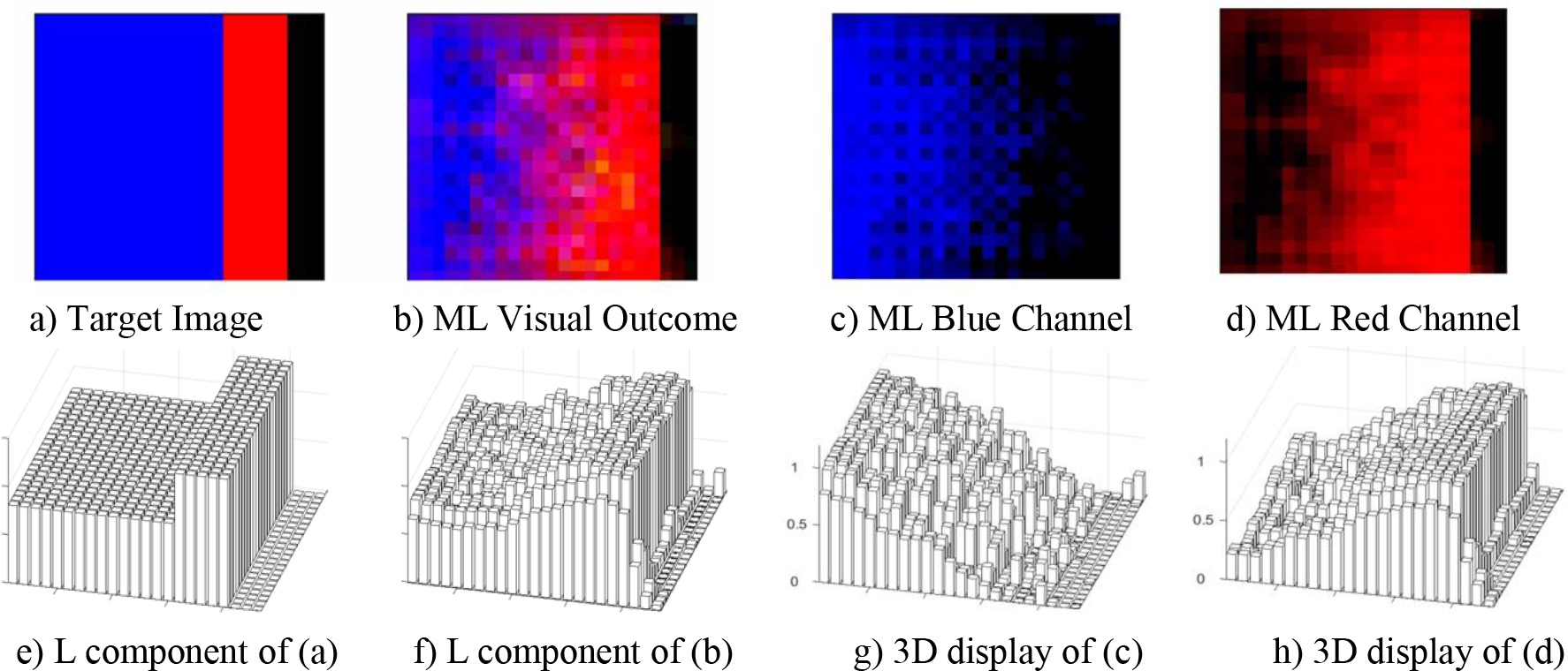
3D Display of the RGB channels of an MCI case that transitioned to AD at T24(24^th month). Note the gradual change in the ML generated displays. Also note how minimally the ML model affected the region of uncertainty (RU) in the 3D displays in f, g and h.

Figure 5.

3D Display of the RGB channels of cases (a), (b), (h) and (u) from Fig. 3. Also note the minimal effects on the region of uncertainty (RU).

4. Discussion

The results of ML4VisAD’s implementation show the need for deep reflection when assessing multiclass classification or prediction results using machine learning, especially when observing all the subtle nuances of the visual outcome. There were a few cases where the ML4VisAD visual output seemed to make more sense than what the target images portrayed, especially concerning the available measurements at the different time points. Case (j) shows a subject that transitioned back to normal control (CN) from an MCI diagnosis in the previous three time points. The ML model did not see it the same way and had the subject as stable CN through all four time points, and most measurements support this classification. Another example is case (l), where the target shows a transition from MCI to AD in T24, while the ML4VisAD visual output displays a stable MCI through all time points. Here again, the measurements are somewhat ambiguous but more in favor of the ML model in that the MMSE did drop but only by one point in T24 compared to T6, and the CDR-SB scores are otherwise consistent through T6 to T24 with the SUVR also consistent in T0 and T24. Another interesting case is (v), where the target image shows a stable MCI, while the ML4VisAD visual output places this subject as stable CN. In this case, from the high MMSE score, the low SUVR values, and an APOE of 0, although the CDR is 0.5, the ML visual outcome of a stable CN seems more reasonable. But other cognitive tests (ADAS, RAVLT) may have influenced the diagnosis, and these scores were not used in the ML4VisAD model to avoid bias. In many of these cases, there may be some merits in generating a composite score, as proposed in [46]. Moreover, for cases (u), (v), and (w), all stable cases misclassified as another type of stable cases, there seems to be an influence of the APOE value on the ML4VisAD outcome (0 influences the CN state, 2 switched CN to MCI, and 1 reverted AD to MCI). See also findings reported in [53].

These ML visual outcomes clearly show why clinicians face difficulty each time they deliberate on a patient’s disease state. For example, it is hard to understand why the subject in case (u) in Figure 3 had an MMSE score of 29 for T0, T12, and T24 but an MMSE score of 24 at time T6. Also, for the same patient in (u) the CDR score was 1 at T0 and reverted to 0 for all subsequent time points. Although the diagnosis is that of a stable CN for (u), the machine learning visual outcome places this subject as stable MCI when considering all other features. Recall that the APOE for (u) is 2 at baseline and that the SUVRs are relatively high. Also, the high number of years of education for this subject (17) may have led to the high MMSE scores of 29 for T0, T12, and T24, although stumbling in the test given at T6.

The subtle nuances encountered with the ML4VisAD visual outcomes could reduce the misclassifications with added scrutiny on the visual output in context to specific measurements clinicians may be interested in. Consequently, the first point is that multiclass classification, whether it is automated or made through a rating process, does not allow for a more thorough deliberation process if these nuances and subtle differences cannot be visually observed and would be so hard to decipher otherwise through tabulated data or decisional spaces showing different overlapped regions among the considered classes. Therefore, it is no revelation that the more classes considered in a multiclass classification algorithm, the less accurate will the classification results be.

4.1. Future Work

The proposed visual outcome enhances the processes of multiclass classification and disease projection with the ability to visualize the inner workings of the machine learning and observe what the differences between the ML visual outcome and target image could mean. In other words, the difference between them does not necessarily mean an outright misclassification but emphasizes the nuances between them and implies that a review is necessary of what may have led to such change, especially if the region of uncertainty (RU) in the visual display remains unaffected.

It is thus essential to recognize that the interrelatedness in features, along with the many variations of such multimodal features, some being temporal, others structural, functional, metabolic, genetic, demographic, or cognitive are extremely difficult to disentangle, especially when combined with subjective thresholds or ranges of scores such as with SUVRs, MMSE, and CDR-SB. When considering ADNI data, there is an overlap in MMSE scores between CN, MCI, and even AD groups, and the CDR-SB values may resolve this overlap. Still, for an ML model, more datasets are required to learn more of the interplay between such cognitive features, especially when used for baseline diagnosis.

We contend that it is possible to define some objective criteria to quantify the uncertainty of the machine’s estimation per case/patient, which is one of the significant open problems for utilizing AI in medicine. As a good first step, we included in our visual template a black bar that evaluates the amount of uncertainty infused by the machine learning model into the classification/prediction results. But we believe further investigation is needed to better understand this effect. For instance, we could investigate the checkerboard effects observed in cases (b) and (j) to determine what led to their presence. Are these effects due to the convolutions and other calculations performed by the ML model, or are they an indication of some subtle changes in the feature space of that specific patient that were not seen in the training phase?

As for the number of classes considered in the study, the proposed method relied on the three primary RGB colors for the three groups (CN, MCI, AD) available in the dataset. However, suppose additional classes such as EMCI, LMCI, or aMCI are also available. In that case, we could always augment the primary color with the secondary colors of yellow, cyan, and magenta (Y, C, M) on the visual template.

As it stands, from the availability of data, there were nearly four times more MCIs than AD and twice as many MCIs than CNs. Since the input features fed into the ML model were those acquired at baseline, a balance of samples between CN, MCI, and AD groups would be ideal in future implementations. Moreover, although ML4VisAD utilized 1,123 subjects, its efficacy could be enhanced by the availability of a much larger and more balanced dataset if the ML model in the training phase is to capture all the nuances that distinguish the different subgroups. ADRC centers and ADNI, who continue to build a much larger population of the various subgroups for research with balanced data regarding ethnicity and disease state, are crucial to future experimentation.

Conclusion

The genesis of this study was to create a new approach for the visualization-based estimation of disease trajectory to augment the diagnosis and prognosis of AD. A new deep learning (DL) architecture based on Convolutional Neural Networks generates a visual image that portrays AD trajectory in a 2-year longitudinal study using baseline features only. From these baseline features, to avoid bias, we remove all cognitive scores MMSE, CDR-SB, and ADAS from consideration in the design of the ML model as the input features. Target images using different colors define each stage of the disease at the four observation time points (T0, T6, T12, and T24), with T0 being the baseline time point. A unique characteristic of this model is that it is trained with known target images with color-coded diagnoses at all four time points to generate a visual output that predicts disease trajectory based on baseline features only. Since we use only baseline features as input, this design is amenable to cross-sectional and longitudinal studies based on similar datasets. This research could also lead to new insights as to the gradual changes between transition phases as a function of the input feature space considered.

Highlights.

• Development of a first-of-its-kind color-coded visualization mechanism for Alzheimer’s disease diagnosis and prognosis using multimodal medical information fusion.

• Integration of a deep learning model to predict disease trajectory in a visualized form.

• Uncertainty and trustfulness visualization associated with machine learning prediction.

• Confirmed higher preferences in the visualized prediction form and the trustfulness observation via a global online survey analysis.

Appendix

Online Survey using the Qualtrics Platform

We created an online survey using the Qualtrics platform to collect users’ feedback on the practicality of this visualization platform. The objective was to assess the ease with which the user could interpret and understand the visual display. It is also an assessment of how easy it is to remember the visual output and how easy or difficult it is to decide based on the visual display, especially when the output may contain some uncertainty revealed in the black bar. Participants are presented with initial samples to familiarize them with the visualization format and its color coding. We shared the survey on Facebook Ads, LinkedIn, and other social media channels, and 103 individuals responded. The figure below shows the sites of the collected user information.

Among those who responded to the survey, 51.5% were female, and the remaining 47.47% were male. A large majority of participants (81.55%) were between 25 and 44 years of age, with 15.5% identifying themselves as being healthcare professionals or working with the medical industry. An overwhelmingly 82.35% expressed a favorable vote for the ease of memorizing/remembering the outcome through visualization. 83.49% of the participants agree that the visual representation is easy to remember, with 79.55% stating that they prefer receiving the results in a visual format. Moreover, 73.79% agreed that the visualized output image speeds up decision-making. As for the level of uncertainty, 81.65% stated that different uncertainty levels are visible in the visualized format.

The following questions were posed, and the results of the survey are as follows:

Q1: Suppose that the state of the disease is displayed in different colors:

• Green: healthy individual

• Blue: moderately diseased patient

• Red: severely diseased patient

In addition, we display the trajectories of disease progression over the four time points by a sequence of 4 color stripes. For example, in the following image:

Is it easy to remember how to interpret the outcome?

The following image shows the outcomes of the algorithm for 4 patients, a to d.

Q2: Is it easy to determine disease progression for each patient?

Q3: Which type of outcomes do you prefer to be presented by an algorithm? (Algorithm A or B?)

Q4: Which type of outcome is more memorable/recall-able? (Algorithm A or B?)

Q5: Which type of outcomes is faster for you to make a decision? (Algorithm A or B?)

Q6: Do you think different level of uncertainty is observable between each pairs of (a,b) and (c,d)?

References

- 1.Lynch M, Alzheimer’s Association, “New Alzheimer’s Association Report Reveals Sharp Increases in Alzheimer’s Prevalence, Deaths and Cost of Care”, Alzheimer’s Association 2018. report, https://www.alz.org/news/2018/new_alzheimer_s_association_report_reveals_sharp_i. [Google Scholar]
- 2.Einav L, Finkelstein A, Mullainathan S, Obermeyer Z, “Predictive modeling of U.S. health care spending in late life”, Science, Vol. 360 (6396), pp. 1462–1465, June 2018. [DOI] [PMC free article] [PubMed] [Google Scholar]
- 3.Scheltens P, Blennow K, Breteler MMB, de Strooper B, Frisoni GB, Salloway S, Van der Flier WM, “Alzheimer’s disease”, Lancet, Vol. 388 (10043), pp. 505–517, July 2016. [DOI] [PubMed] [Google Scholar]
- 4.Young PNE, Estarellas M, Coomans E, et al.” Imaging biomarkers in neurodegeneration: current and future practices”, Alzheimers Research & Therapy, Vol. 12 (1), Article No: 49, April 27, 2020. [DOI] [PMC free article] [PubMed] [Google Scholar]
- 5.Jack, CR CR, Knopman DS, Jagust WJ, Petersen RC, Weiner MW, Aisen PS, Shaw LM, Vemuri P, et al. , “Tracking pathophysiological processes in Alzheimer’s disease: an updated hypothetical model of dynamic biomarkers”, Lancet Neurology, Vol. 12 (2), pp. 207–216, Feb 2013. [DOI] [PMC free article] [PubMed] [Google Scholar]
- 6.Loewenstein DA, Curiel RE, DeKosky S, Bauer RM, Rosselli M, Guinjoan SM, Adjouadi M Peñate MA, Barker WW, Goenaga S, Golde T, Greig-Custo MT, Hanson KS, Li C, Lizarraga G, Marsiske M, and Duara R, “Utilizing semantic intrusions to identify amyloid positivity in mild cognitive impairment”, Neurology, Vol. 27 (11), pp. E976–E984, September 2018. [DOI] [PMC free article] [PubMed] [Google Scholar]
- 7.Selkoe DJ, “Early network dysfunction in Alzheimer’s disease”, Science, 365 (6453), pp. 540–541, August 2019. [DOI] [PubMed] [Google Scholar]
- 8.Jessen F, Amariglio RE, Buckley RF, et al. , “The characterisation of subjective cognitive decline”, Lancet Neurology, Vol. 19 (3), pp. 271–278, Marcgh 2020. [DOI] [PMC free article] [PubMed] [Google Scholar]
- 9.van Loenhoud AC, van der Flier WM, Wink AM, Dicks E, Groot C, Twisk J, Barkhof F, Scheltens P, Ossenkoppele R, for the Alzheimer’s Disease Neuroimaging Initiative, “Cognitive reserve and clinical progression in Alzheimer disease: A paradoxical relationship”, Neurology. 2019. Jul 23; 93(4): e334–e346. [DOI] [PMC free article] [PubMed] [Google Scholar]
- 10.Nortley R, Korte N, Izquierdo P, Hirunpattarasilp C, Mishra A, Jaunmuktane Z, Kyrargyri V et al. , “Amyloid beta oligomers constrict human capillaries in Alzheimer’s disease via signaling to pericytes”, Science, Vol. 365 (6450), 11 pages, July 2019. [DOI] [PMC free article] [PubMed] [Google Scholar]
- 11.Scholl M and Maass A, “Does early cognitive decline require the presence of both tau and amyloid-beta?”, Brain, Vol. 143, pp: 10–13, Part: 1, January 2020. [DOI] [PubMed] [Google Scholar]
- 12.Lockhart SN, Scholl M, Baker SL, et al. , “Amyloid and tau PET demonstrate region-specific associations in normal older people”, NeuroImage, Vol. 150, pp. 191–199, April 2017. [DOI] [PMC free article] [PubMed] [Google Scholar]
- 13.Montagne A, Nation DA, Sagare AP, Barisano G, Sweeney MD, Chakhoyan A, Pachicano M, Joe E, Nelson AR, D’Orazio LM, et al. ,” APOE4 leads to blood-brain barrier dysfunction predicting cognitive decline”, Nature, Vol. 581, pp. 71–76, April 2020. [DOI] [PMC free article] [PubMed] [Google Scholar]
- 14.Li T, Wang B, Gao Y, Wang X, Yan T, Xiang J, et al. ,” APOE epsilon 4 and cognitive reserve effects on the functional network in the Alzheimer’s disease spectrum”, Brain Imaging and Behavior, DOI: 10.1007/s11682-020-00283-w, Early Access, 2020 [DOI] [PubMed] [Google Scholar]
- 15.Therriault, Joseph J; Benedet AL, Pascoal TA, Tharick A, Mathotaarachchi S, Chamoun M, Savard M, et al. , “Association of Apolipoprotein E epsilon 4 With Medial Temporal Tau Independent of Amyloid-beta,”JAMA Neurology, Vol. 77 (4), pp. 470–479, April 2020. [DOI] [PMC free article] [PubMed] [Google Scholar]
- 16.Olsson B, Lautner R, Andreasson U, et al. ,” CSF and blood biomarkers for the diagnosis of Alzheimer’s disease: a systematic review and meta-analysis”, Lancet Neurology, Vol. 15 (7), pp. 673–684, June 2016. [DOI] [PubMed] [Google Scholar]
- 17.Lewczuk P, Matzen A, Blennow K, Parnetti L, Molinuevo JL, Eusebi P, et al. ,” Cerebrospinal Fluid A beta(42/40) Corresponds Better than A beta(42) to Amyloid PET in Alzheimer’s Disease,”Journal of Alzheimers Disease, Vol. 55 (2), pp. 813–822, 2017. [DOI] [PMC free article] [PubMed] [Google Scholar]
- 18.Sabbagh M, Sadowsky C, Tousi B, Agronin ME, Alva G, Armon C, Bernick C, Keegan AP, Karantzoulis S, Baror E, et al. , “Effects of a combined transcranial magnetic stimulation (TMS) and cognitive training intervention in patients with Alzheimer’s disease”, Alzheimers & Dementia, Vol. 16 (4), pp. 641–650, April 2020 [DOI] [PubMed] [Google Scholar]
- 19.Romanella M, Roe D, Paciorek R, Cappon D, Ruffini G, Menardi A, Rossi A, Rossi S, Santarnecchi E, “Sleep, Noninvasive Brain Stimulation, and the Aging Brain: Challenges and Opportunities”, Ageing Research Reviews, Vol. 61, Article No: 101067, August 2020. [DOI] [PMC free article] [PubMed] [Google Scholar]
- 20.Tăuţan AM, Ionescu B, Santarnecchi E, “Artificial intelligence in neurodegenerative diseases: A review of available tools with a focus on machine learning techniques.” Artificial Intelligence in Medicine. 2021. [DOI] [PubMed] [Google Scholar]
- 21.Khojaste-Sarakhsi M, Haghighi SS, Ghomi SF, Marchiori E, “Deep learning for Alzheimer’s disease diagnosis: A survey.” Artificial Intelligence in Medicine. 2022 [DOI] [PubMed] [Google Scholar]
- 22.Pellegrini E, Ballerini L, Valdes Hernandez MC, Chappell FM, González-Castro V, Anblagan D, et al. “Machine learning of neuroimaging for assisted diagnosis of cognitive impairment and dementia: A systematic review. Alzheimer’s & Dementia: Diagnosis, Assessment & Disease Monitoring Vol. 10, pp. 519–535, 2018. [DOI] [PMC free article] [PubMed] [Google Scholar]
- 23.Ezzati A, Zammit AR, Harvey DJ, et al. , “Optimizing Machine Learning Methods to Improve Predictive Models of Alzheimer’s Disease”, Journal of Alzheimers Disease, Vol. 71 (3), pp. 1027–1036, 2019. [DOI] [PMC free article] [PubMed] [Google Scholar]
- 24.Tabarestani S, Aghili M, Eslami M, Cabrerizo M, Barreto A, Rishe N, Curiel RE, Loewenstein D, Duara R, Adjouadi M, “A Distributed Multitask Multimodal Approach for the Prediction of Alzheimer’s Disease in a Longitudinal Study”, NeuroImage, Vol. 206, Article No: 116317, February 2020. [DOI] [PMC free article] [PubMed] [Google Scholar]
- 25.Donini M, Monteiro JM, Pontil M, Hahn T, Fallgatter AJ, Shawe-Taylor J, Mourão-Miranda J, “Combining heterogeneous data sources for neuroimaging based diagnosis: re-weighting and selecting what is important”, NeuroImage, Vol. 195, pp. 215–231, July 2019. [DOI] [PMC free article] [PubMed] [Google Scholar]
- 26.Tabarestani S, Eslami M, Cabrerizo M, Barreto A, Rishe N, Curiel RE, Barreto A, Rishe N, Vaillancourt D, DeKosky ST, Loewenstein DA, Duara R, Adjouadi M, “A Tensorized Multitask Deep Learning Network for Progression Prediction of Alzheimer’s Disease”, Frontiers in Aging Neuroscience, Vol. 14, Article Number: 810873, DOI: 10.3389/fnagi.2022.810873, May 2022. [DOI] [PMC free article] [PubMed] [Google Scholar]
- 27.Shojaie M, Tabarestani S, Cabrerizo M, DeKosky ST, Vaillancourt DE, Loewenstein D, Duara R, and Adjouadi M, “PET Imaging of Tau Pathology and Amyloid-β, and MRI for Alzheimer’s Disease Feature Fusion and Multimodal Classification”, Journal of Alzheimer’s Disease, Vol. 84 (4), pp. 1497–1514, 2021. 10.3233/JAD-210064. [DOI] [PMC free article] [PubMed] [Google Scholar]
- 28.Ranjbarzadeh R, Caputo A, Tirkolaee EB, Ghoushchi SJ, Bendechache M, “Brain tumor segmentation of MRI images: A comprehensive review on the application of artificial intelligence tools”, Computers in Biology and Medicine, Vol. 152, January 2023, 106405. [DOI] [PubMed] [Google Scholar]
- 29.Aghamohammadi A, Ranjbarzadeh R, Naiemi F, Mogharrebi M, Dorosti S, Bendechache M, “TPCNN: Two-path convolutional neural network for tumor and liver segmentation in CT images using a novel encoding approach”, Expert Systems with Applications, Vol. 183, 30 November 2021, 115406 [Google Scholar]
- 30.Kazeminia S, Baur C, Kuijper A, van Ginneken B, Navab N, Albarqouni S, Mukhopadhyay A, “GANs for medical image analysis”, Artificial Intelligence in Medicine, DOI: 10.1016/j.artmed.2020.101938, Aug. 2020. [DOI] [PubMed] [Google Scholar]
- 31.Bruno P, Calimeri F, Kitanidis AS, De Momi E, “Data reduction and data visualization for automatic diagnosis using gene expression and clinical data, Artificial Intelligence in Medicine, Vol.107, Article Number 101884, DOI: 10.1016/j.artmed.2020.101884, JUL 2020. [DOI] [PubMed] [Google Scholar]
- 32.Lizarraga G, Li C, Cabrerizo M, Barker W, Loewenstein DA, Duara R, and Adjouadi M, “A Neuroimaging Web Services Interface as a Cyber Physical System for Medical Imaging and Data Management in Brain Research: Design Study” JMIR Medical Informatics, Vol. 6 (2), pp. 228–244, Apr-Jun 2018. [DOI] [PMC free article] [PubMed] [Google Scholar]
- 33.Yuan J, Sartor EA, Au R, B Kolachalama V, “Development and validation of an interpretable deep learning framework for Alzheimer’s disease classification”, Brain, 143(6):1920–1933, doi: 10.1093/brain/awaa137, June 2020. [DOI] [PMC free article] [PubMed] [Google Scholar]
- 34.Li Qi, “Overview of Data Visualization”, Embodying Data. 17–47. Published online 2020 Jun 20. doi: 10.1007/978-981-15-5069-0_2, June 2020. [DOI] [Google Scholar]
- 35.Seo K, Pan R, Lee D, Thiyyagura P, Chen K, “Visualizing Alzheimer’s disease progression in low dimensional manifolds”, Heliyon. Vol. 5(8): e02216, August 2019. [DOI] [PMC free article] [PubMed] [Google Scholar]
- 36.Blanken AE, Jang JY, Ho JK, Edmonds EC, Han SD, Bangen KJ, Nation DA, “Distilling Heterogeneity of Mild Cognitive Impairment in the National Alzheimer Coordinating Center Database Using Latent Profile Analysis”, JAMA Network Open, Vol. 3 (3), March 2020. [DOI] [PMC free article] [PubMed] [Google Scholar]
- 37.Liu X, Tosun D, Weiner MW, Schuff N, “Locally Linear Embedding (LLE) for MRI based Alzheimer’s Disease Classification”, NeuroImage, Vol. 83, pp. 148–157, December 2013. [DOI] [PMC free article] [PubMed] [Google Scholar]
- 38.Gerber S, Tasdizen T, Fletcher PT, Joshi S, Whitaker R, “Manifold modeling for brain population analysis” Medical Image Analysis, Vol. 14 (5), pp. 643–653, October 2010. [DOI] [PMC free article] [PubMed] [Google Scholar]
- 39.Berron D, van Westen D, Ossenkoppele R, Strandberg O, Hansson O, “Medial temporal lobe connectivity and its associations with cognition in early Alzheimer’s disease”, Brain, Vol. 143(4), pp. 1233–1248, April 2020. [DOI] [PMC free article] [PubMed] [Google Scholar]
- 40.Montez T, Simon-Shlomo Poil, Jones BF, Manshanden I, Verbunt JPA, van Dijk BW, Brussaard AB, van Ooyen A, Stam CJ, Scheltens P, Linkenkaer-Hansen K, “Altered temporal correlations in parietal alpha and prefrontal theta oscillations in early-stage Alzheimer disease”, Proc Natl Acad Sci U S A. Vol. 106(5), pp. 1614–1619, February 2009. [DOI] [PMC free article] [PubMed] [Google Scholar]
- 41.Buckley RF, Schultz AP, Hedden T, Papp KV, Hanseeuw BJ, Marshall G, Sepulcre J, Smith EE, et al. , “Functional network integrity presages cognitive decline in preclinical Alzheimer disease”, Neurology, Vol. 89(1), pp. 29–37, July 2017. [DOI] [PMC free article] [PubMed] [Google Scholar]
- 42.Wisch JK, Roe CM, Babulal GM, Schindler Su. E., Fagan AM, Benzinger TL, Morris JC, Ances BM, “Resting State Functional Connectivity Signature Differentiates Cognitively Normal from Individuals Who Convert to Symptomatic Alzheimer Disease”, J Alzheimers Dis, Vol. 74(4), pp. 1085–1095, 2020. [DOI] [PMC free article] [PubMed] [Google Scholar]
- 43.Toddenroth D, Ganslandt T, Castellanos I, Prokosch HU, Barkle T, “Employing heat maps to mine associations in structured routine care data”, Artificial Intelligence In Medicine, Vol. 60 (2) 2 Pages: 79–88, February 2014. [DOI] [PubMed] [Google Scholar]
- 44.Klemm P, Lawonn K, Glasser S, Niemann U, Hegenscheid K, Volzke H, Preim B, “3D Regression Heat Map Analysis of Population Study Data”, IEEE Trans. on Visualization and Computer Graphics, Vol. 22 (1), pp. 81–90, January 2016. [DOI] [PubMed] [Google Scholar]
- 45.Qiu S, Joshi PS, Miller MI, Xue CH “Development and validation of an interpretable deep learning framework for Alzheimer’s disease classification”, Brain, Vol. 143 (6), pp. 1920–1933, June 2020. [DOI] [PMC free article] [PubMed] [Google Scholar]
- 46.Jelistratova I, Teipel SJ, Grothe MJ, Michel J, “Longitudinal validity of PET-based staging of regional amyloid deposition”, Human Brain Mapping, DOI: 10.1002/hbm.25121, Early Access: July 2020. [DOI] [PMC free article] [PubMed] [Google Scholar]
- 47.Ossenkoppele R, Jansen WJ, Rabinovici GD, Knol DL, van der Flier WM, M van Berckel BN, Scheltens P, Visser PJ, “Prevalence of Amyloid PET Positivity in Dementia Syndromes A Meta-analysis” JAMA-Journal Of The American Medical Association, Vol. 313 (19), pp. 1939–1949, May 2015. [DOI] [PMC free article] [PubMed] [Google Scholar]
- 48.Landau SM, Breault C, Joshi AD, Pontecorvo M, Mathis CA, Jagust WJ, Mintun MA, “Amyloid-β Imaging with Pittsburgh Compound B and Florbetapir: Comparing Radiotracers and Quantification Methods”, J Nuclear Medicine. Vol. 54(1), pp. 70–77, January 2013. [DOI] [PMC free article] [PubMed] [Google Scholar]
- 49.J Grothe M, Barthel H, Sepulcre J, Dyrba M, Sabri O, J Teipel S, “In vivo staging of regional amyloid deposition”, Neurology, Vol. 89(20), pp. 2031–2038, November 2017. [DOI] [PMC free article] [PubMed] [Google Scholar]
- 50.Parbo P, Ismail R, Hansen KV, Amidi A, Mårup FH, Gottrup H, Brændgaard H, Eriksson BO, Eskildsen SF, Lund TE, et al. , “ Brain inflammation accompanies amyloid in the majority of mild cognitive impairment cases due to Alzheimer’s disease”, Brain, Vol. 140 (7), pp, 2002–2011, May 2017 [DOI] [PubMed] [Google Scholar]
- 51.Duara R R, Loewenstein DA, Lizarraga G, Adjouadi M, Barker WW, Greig-Custo MT, Rosselli M M, Penate A, Shea YF, Behar R, Ollarves A, Robayo C, Hanson K, Marsiske M, Burke S, Ertekin-Taner N, Vaillancourt D, De Santi S, Golde T, “Effect of age, ethnicity, sex, cognitive status and APOE genotype on amyloid load and the threshold for amyloid positivity”, Neuroimage Clinical Vol. 22, Article Number: UNSP 101800, 2019. [DOI] [PMC free article] [PubMed] [Google Scholar]
- 52.Qiu S, Joshi PS, Miller MI, Xue CH “Development and validation of an interpretable deep learning framework for Alzheimer’s disease classification”, Brain, Vol. 143 (6), pp. 1920–1933, June 2020. [DOI] [PMC free article] [PubMed] [Google Scholar]
- 53.Crane PK, Carle A, Gibbons LE, Insel P, Mackin RS, Gross A, Jones RN, Mukherjee S, Curtis SM, Harvey D, Weiner M, and Mungas, for the Alzheimer’s Disease Neuroimaging Initiative, “Development and assessment of a composite score for memory in the Alzheimer’s Disease Neuroimaging Initiative (ADNI), Brain Imaging Behav. 2012. Dec; 6(4): 502–516. [DOI] [PMC free article] [PubMed] [Google Scholar]
- 54.Liu M, Zhang J, Adeli E, Shen D (2018c). Joint classification and regression via deep multi-task multi-channel learning for Alzheimer’s disease diagnosis. IEEE Trans. Biomed. Eng. 66 1195–1206. 10.1109/TBME.2018.2869989. [DOI] [PMC free article] [PubMed] [Google Scholar]
- 55.Zhu X, Suk H-I, Lee S-W, Shen D (2016a). Canonical feature selection for joint regression and multi-class identification in Alzheimer’s disease diagnosis. Brain Imaging Behav. 10 818–828. 10.1007/s11682-015-9430-9434. [DOI] [PMC free article] [PubMed] [Google Scholar]
- 56.Shi J, Zheng X, Li Y, Zhang Q, Ying S (2018). Multimodal neuroimaging feature learning with multimodal stacked deep polynomial networks for diagnosis of Alzheimer’s disease. IEEE J. Biomed. Health Inform. Vol. 22 (1), pp.173–183. 10.1109/JBHI.2017.2655720. [DOI] [PubMed] [Google Scholar]
- 57.Lin WM, Gao QQ, Tong T, “Multiclass diagnosis of stages of Alzheimer’s disease using linear discriminant analysis scoring for multimodal data”, Computers in Biology and Medicine, Vol. 134, Article Nb 104478, Jul 2021. [DOI] [PubMed] [Google Scholar]
- 58.Fang C, Li C, Forouzannezhad P, Cabrerizo M, Curiel RE, Loewenstein D, Duara R, Adjouadi M, “Gaussian Discriminative Component Analysis for Early Detection of Alzheimer’s Disease: A Supervised Dimensionality Reduction Algorithm”, Journal of Neuroscience Methods, Vol. 344, Article 108856, October 2020. [DOI] [PMC free article] [PubMed] [Google Scholar]
- 59.‘Bryant SE, Waring SC, Cullum CM, et al. Staging Dementia Using Clinical Dementia Rating Scale Sum of Boxes Scores: A Texas Alzheimer’s Research Consortium Study. Arch Neurol. 2008;65(8):1091–1095. doi: 10.1001/archneur.65.8.1091 [DOI] [PMC free article] [PubMed] [Google Scholar]