Quantitative fluorescence emission anisotropy microscopy for implementing homo–fluorescence resonance energy transfer measurements in living cells

Abstract

Quantitative fluorescence emission anisotropy microscopy reveals the organization of fluorescently labeled cellular components and allows their characterization in terms of changes in either rotational diffusion or homo-Förster’s energy transfer characteristics in living cells. These properties provide insights into molecular organization, such as orientation, confinement, and oligomerization in situ. Here we elucidate how quantitative measurements of anisotropy using multiple microscope systems may be made by bringing out the main parameters that influence the quantification of fluorescence emission anisotropy. We focus on a variety of parameters that contribute to errors associated with the measurement of emission anisotropy in a microscope. These include the requirement for adequate photon counts for the necessary discrimination of anisotropy values, the influence of extinction ratios of the illumination source, the detector system, the role of numerical aperture, and excitation wavelength. All these parameters also affect the ability to capture the dynamic range of emission anisotropy necessary for quantifying its reduction due to homo-FRET and other processes. Finally, we provide easily implementable tests to assess whether homo-FRET is a cause for the observed emission depolarization.

INTRODUCTION

Fundamental processes of intracellular life may be understood in terms of pools of molecules that diffuse, interact, bind, change conformation, and catalyze physical and chemical state changes within the confined volume of a cell. Utilizing the arsenal of available techniques allows the researcher to unravel rules that govern these processes (van Zanten and Mayor, 2015). Traditional biochemical methods (grind and find) provide ensemble averages of concentrations as well as information on interacting species, but lack access to spatial information at the scale of the processes carried out inside the cell. Chemical specific spatial contrast is achieved by using tagged markers in combination with imaging. In a fluorescence setting, optically resolved spatial information can be coupled with high temporal resolution and high signal-to-noise ratio (SNR) in living systems. However, far field–based fluorescence techniques are inherently diffraction-limited, and following individual proteins at a density above 10 per μm² becomes difficult (Jaqaman et al., 2008; Manley et al., 2008; Sergé et al., 2008). Therefore, it remains challenging to provide direct in situ evidence of interaction, binding, and conformational changes of molecules under physiological conditions.

Forsters or fluorescence resonance energy transfer (FRET) is uniquely sensitive to the detection of short-length interactions between fluorophores. This allows a window on events that occur at range 1–10 nm, even though diffraction-limited imaging systems are used (Krishnan et al., 2001). Depending on several important conditions (such as spectral overlap, the distance between, and the orientation of the fluorophore dipoles) that have been documented previously (Jares-Erijman and Jovin, 2003), two spectrally distinct fluorophores can transfer the energy of the excited-state donor (blue-shifted) fluorophore to the acceptor (red-shifted) fluorophore (Hoppe et al., 2002) in a nonradiative process called hetero-FRET. This concomitantly occurs with a decrease in the donor fluorophore lifetime (Wallrabe and Periasamy, 2005). The sensitivity of this process to the fluorophore distance at the nanometer scale invokes the adage of a spectroscopic ruler (Stryer, 1978). An increase in FRET is additionally associated with a depolarization of the emission if donor fluorophores are excited with polarized light (Förster, 1948). Especially when donor and acceptor are on different molecules (Rizzo et al., 2006), the polarization-based method benefits from a large dynamic range and reduced background from the acceptor fluorophore (Sharma et al., 2004; Rizzo and Piston, 2005). However, the ratio between donor and acceptor fluorophores influences the dynamic range and sensitivity of the hetero-FRET process.

FRET between like fluorophores, called homo-FRET, also takes place. Instead of measuring the changes in the lifetime of the donor or the spectral shift of the detected fluorescence, the extent of homo-FRET is determined by measuring the reduction in emission polarization anisotropy (Weber, 1954; Lidke et al., 2003). The homo-FRET methodology eliminates the requirement for careful tuning of donor–acceptor ratios. Consequently, the method is advantageous for detecting homooligomerization even when only a very small fraction of interacting species are present (Varma and Mayor, 1998; Sharma et al., 2004). This permits a measurement of oligomerization below the detection limit of hetero-FRET labeling techniques (Kenworthy and Edidin, 1998; Sharma et al., 2004). Here, we provide a systematic way to perform steady-state homo-FRET measurements, and a comprehensive and practical compendium for the use of emission anisotropy for the detection of homo-FRET. We document factors that will affect the dynamic range of the measurement, as well as measurement-associated errors, and suggest ways to attribute the anisotropy measurement to homo-FRET. This will allow a rigorous and quantitative implementation of this powerful technique in biological systems where such resolution is necessary.

RESULTS

Measuring homo-FRET: Theoretical background

The magnitude of homo-FRET may be determined by measuring the extent of depolarization of fluorescence emission (or reduction in emission anisotropy) upon exciting fluorophores with polarized light (Lakowicz, 2006). In this photophysical process, fluorophore dipoles that are aligned parallel to the plane of polarization of the excitation beam are excited. Fluorescence emission anisotropy, r, is detected by collecting emitted photons at two orthogonal polarizations. A schematic depicting the main characteristics of an anisotropy microscope is shown in Figure 1A.

FIGURE 1:

Concept and experiments displaying examples of polarized fluorescence emission anisotropy. (A) A schematic of the core elements of fluorescence anisotropy microscopy. Polarized excitation is directed to the sample through an objective, which also collects the resulting fluorescence emission. After appropriate wavelength filtering, the emission light of unknown polarization is separated into two orthogonal polarization channels (POL BS): one parallel to the excitation polarization and the other perpendicular. (B) Whether at the plasma membrane (lipid bilayer) or in the cytosol of a cell (gray region), fluorophores that have their dipoles aligned with the excitation polarization become excited through photoselection. (i) A fluorophore with limited rotational mobility during its fluorescence lifetime, such as typical fluorescent protein, will emit a photon that has polarization aligned to the excitation polarization. (ii) Smaller molecules can rotate much faster and depolarize their emission with respect to the excitation polarization. (iii) If the energy is transferred to a nearby fluorophore, the resulting emitted photon will be depolarized with respect to the excitation polarization, because the second fluorophore is more likely to be differently oriented with respect to the first fluorophore. (C) Experimental data showing the effect of fluorescence lifetime and rotational time on the steady-state emission anisotropy measurement. Anisotropy increases as the rotational timescale is slowed down through increasing the viscosity of the solution by increasing the glycerol content (x-axis, from 10^–3 Pa·s to 1.412 Pa·s) or due to a size increase of the fluorophore (EGFP versus Rho6G; M_w of 26.9 kDa versus 0.8 kDa resulting in a φ of 14 ns versus 0.12 ns). The influence of fluorescence lifetime is exemplified by the higher anisotropy of Cy3 than of Rho6G due to the shorter lifetime of Cy3 (τ = 0.3 ns versus τ = 3.43 ns). (D) Experimental data displaying the effect of molecular proximity on the anisotropy measurement. Concentration-dependent anisotropy of Rho6G in a 70% glycerol solution (∼2.3 × 10^–2 Pa·s) contains two regimes: (1) a regime determined only by rotational diffusion and (2) a regime where Rho6G is undergoing increasing collisional homo-FRET upon an increasing concentration (above 100 µM).

The following expression is used to define fluorescence anisotropy:

1

where I_|| and I_⊥ are the detected emission intensities parallel and perpendicular to the excitation, respectively. G is the g-factor of the microscope, defined as the detection efficiency of the parallel polarized photons with respect to the perpendicular polarized photons. The denominator in Eq. 1 is equivalent to the total number of photons detected, making it possible to compare anisotropy values from heterogeneous regions. In other words, the detected anisotropy is the fractional sum of anisotropies originating from the region of measurement. For an ensemble of immobile but isotropically oriented fluorophores that have their emission dipoles aligned with their absorption dipoles (Figure 1Bi), the maximum attainable anisotropy for single-photon excitation is 0.4. Angular mismatch between the absorption and emission dipoles, β, results in instantaneous depolarization and determines the fluorophore-dependent intrinsic anisotropy, r₀, which is lower than 0.4 (e.g., GFP: β = 11°, r₀ = 0.389 (Myšková et al., 2020)).

For fluorophores that can rotate freely, the extent of depolarization with respect to the excitation is described by the Perrin equation that relates the fluorescence anisotropy to both the fluorescence lifetime and the rotational diffusion time of the fluorophore (Perrin, 1926; Figure 1Bii):

2

where τ is the fluorescence lifetime of the fluorophore and φ is the rotational time constant. For the small fluorophore Rho6G, its lifetime of 3.43 ns is much longer than its rotational diffusion in water (φ ∼ 0.12 ns). In essence, this means that the emission dipole of an excited Rho6G molecule has had time to randomly reorient many times before emitting a photon, resulting in a measured anisotropy close to 0 (Figure 1C). An increased anisotropy is obtained for fluorophores that have either a reduced fluorescence lifetime comparable to their rotational timescale, such as Cy3, (τ ∼ 0.3 ns, Figure 1C) or an increased rotational timescale, such as EGFP (φ ∼ 17 ns, Figure 1C).

Increasing the viscosity of the solution increases the rotational diffusion time of a fluorophore. Figure 1C shows that increasing the fraction of glycerol in the solution results in an increase in anisotropy for all three fluorophores (Rho6G, Cy3, and EGFP). Note that the measured anisotropy of Rho6G almost completely covers the full dynamic range expected from an ensemble of molecules rotating rapidly with respect to their lifetime to one randomly oriented in the static limit, where the rotational diffusion is very slow compared with the lifetime of the fluorophore. The emission anisotropy values range from 0 to 0.35, likely limited through instantaneous depolarization due to the angular difference discussed above. Although not usually taken into account, it is worthwhile to consider the refractive index of the medium. The lifetime of many fluorophores is sensitive to changes in refractive index (Strickler and Berg, 1962; Suhling et al., 2002; τ ∝ η⁻², where η is the refractive index). Taking a look at Eq. 2, it is evident that as refractive index increases, the anisotropy will also increase. Changes in the refractive index may come about by differences in material chemistry or an increase in macromolecular crowding, which is a common state in intracellular conditions (Boersma et al., 2015; van den Berg et al., 2017). Reported variation in the subcellular refractive index can range from 1.1 to 1.5 (Zhang et al., 2017), which can bring about a 10% variation of the anisotropy value measured from cytosolic GFP (r = 0.33–0.36).

These influences on the value of anisotropy are realized in situations where the fluorophores are dilute and hence far apart from each other. With increasing concentration, intermolecular distances decrease, bringing fluorophores within Förster’s radius, where Förster’s resonance energy transfer takes place. In this process, energy from one fluorophore may be transferred nonradiatively to a nearby fluorophore (Figure 1Biii). Since the emission dipole of this second fluorophore will be oriented stochastically with respect to the absorption dipole of the first, energy transfer effectively depolarizes the emission from the interacting pair of fluorophores. This depolarization or decrease in anisotropy provides a measure of the efficiency of the energy transfer process,

3

where r_∞ is the anisotropy of the fluorophore at infinite dilution and E_FRET is the energy transfer efficiency. In a dilute solution r_∞ is described by the Perrin equation, and E_FRET values will rise once the fluorophores in solution start approaching each other at distances, d, comparable or closer than Förster’s radius:

4

Förster’s radius, R₀, measured in Å is defined as the distance between two fluorophores for which the energy transfer is 50% (Förster, 1948):

5

where J(λ) is the spectral overlap between donor emission and acceptor excitation, n is the refractive index of the medium in the range of spectral overlap, Q_D is the quantum yield of the donor in the absence of an acceptor, and κ is the orientation factor between the dipole of two fluorophores (normally assumed to be 2/3, but itcan be measured; Dale et al., 1979).

The effect of collisional homo-FRET can be realized experimentally by measuring the fluorescence emission anisotropy of Rho6G in a 70% glycerol:water solution with increasing Rho6G concentration. Above a concentration of 100 μM, the anisotropy of the solution starts decreasing due to energy transfer between fluorophores (Figure 1D), reflecting the fact that at these concentrations a measurable fraction of molecules are within Förster’s radius of each other. At even higher concentrations, above 2 mM, rhodamine dye molecules start forming highly quenched excited-state species that do not participate in the FRET process, and consequently the anisotropy of the solution increases (Ghosh et al., 2012).

How microscope polarization characteristics affect the anisotropy measurement

Anisotropy measurements in a microscope is easy to set up and implement on any imaging modality available today, provided a few conditions related to preserving the dynamic range of the measurements are fulfilled. Here we outline the conditions that relate to this requirement for emission anisotropy measurements conducted in either confocal, TIFR, or wide-field modalities. In a confocal microscope, emission anisotropy measurements have been implemented in point scanning (Bader et al., 2009), line scanning (Goswami et al., 2008; Ghosh et al., 2012), or light sheet (Hedde et al., 2015; Markwardt et al., 2018), or as a spinning-disk (Ghosh et al., 2012; Gowrishankar et al., 2012) system. The wide-field microscope has been used in an EPI illumination configuration (Varma and Mayor, 1998; Ghosh et al., 2012) or with an appropriate objective in a total internal reflection configuration (Ghosh et al., 2012; Raghupathy et al., 2015; Kalappurakkal et al., 2019). The heart of the measurement lies in the ability to excite fluorophores with polarized light and collect fluorescence emission with sufficiently high polarization extinction ratios (Figure 1A).

To establish the effect of various instrumental parameters, we took advantage of the fact that the difference in anisotropy of a 1-μM Rho6G solution in water from that measured in 100% glycerol covers almost the entire range of emission anisotropy available for a molecule dissolved in a solvent: from 0, as expected from a molecule rotating much faster than its fluorescence lifetime, to 0.35, where the value of anisotropy is a result of the rotationally averaged distribution of dipoles that are excited by polarized light and have a very low rotational diffusion coefficient. First, the excitation polarization extinction ratio (I_||/I_⊥:1) at the sample plane was gradually reduced from 1500:1 to 1:1 using a λ/4 waveplate (Figure 2A). When the polarization extinction ratio was reduced below 150:1, the measured dynamic range started decreasing, setting the minimum requirement for the polarization extinction of the excitation path for maximum dynamic range. Placing a high-quality polarizer (e.g., Newport 10LP-VIS-B or MoxTek PFU04C) in a collimated segment of the excitation path before the sample plane will ensure that this requirement is met.

FIGURE 2:

Effects of polarization characteristics on the dynamic range of an anisotropy experiment. (A) Lowering the excitation polarization extinction ratio by rotating a λ/4 waveplate that is placed in the excitation path dramatically lowers the dynamic range of an anisotropy experiment. The dynamic range is experimentally determined as the difference between Rho6G dissolved in glycerol versus that dissolved in water. (B) The orientation of the polarization of the excitation source can be misaligned with respect to the detection polarization axis by rotating a λ/2 waveplate that is placed in the excitation path. Misalignment significantly reduces the dynamic range, eventually flipping the sign of the anisotropy, because the parallel and perpendicular detection axes with respect to the excitation polarization become interchanged above 45°. (C) The maximum attainable dynamic range is also determined by the polarization extinction ratios (or SNRs) for each of the two detector channels. The dynamic range is most sensitive to the extinction ratio of the parallel channel (x-axis). Nevertheless, to avoid loss of dynamic range (color scale), both the extinction ratios should ideally remain above 100:1. The blue dashed lines indicate a 1% and a 10% loss of dynamic range. (D) The depolarization effect associated with high NA objectives changes the detected anisotropy values and thus the dynamic range. The NA of a microscope system can be changed by using different NA objectives (different colored squares) or by changing the aperture size of a variable-NA objective (black squares). As expected from theory, the dynamic range decreases with increasing NA. The theoretical change in dynamic range is dependent on the refractive index and was adjusted to the mean (blue and black lines for n = 1.0 and n = 1.515, respectively) and SD (blue and black shaded regions) of the measurement using the 10× 0.3 NA objective (see Materials and Methods).

Next, the direction of the maximum polarization extinction ratio (1500:1) was changed with respect to the detection polarizations using a λ/2 waveplate (Figure 2B). A misalignment no more than 5° is necessary to obtain the maximum dynamic range. Note that negative values of anisotropy arise because the parallel and perpendicular detectors become interchanged after 45°. Because high–numerical aperture (NA) objectives scramble the polarization (see below), these polarization calibration measurements were performed using a low-NA-low magnification air objective (10×, 0.3 NA) on an epiilluminated microscope system.

Finally, on the detection side, it is equally important to have a high polarization extinction ratio for each detection channel to obtain the maximum dynamic range in the measurement. The effect of the polarization extinction ratio on each of the detectors can be simulated in terms of bleedthrough (Figure 2C). For example, a 50:1 extinction ratio for the perpendicular channel means a 2% contribution from parallel photons. The result is a reduced effective dynamic range of the anisotropy measurement. The most sensitive detector is the parallel channel, and the dynamic range decreases significantly when its extinction ratio drops below 20:1. One should ideally aim to have extinction ratios greater than 100:1 for both channels. These images may be recorded sequentially using two orthogonally oriented high-quality polarizers or simultaneously by splitting the emission signal using a polarizing beam splitter and collecting the image on one or two cameras (Ghosh et al., 2012). Wire polarizing beam splitters (MoxTek) typically have polarization extinction ratios on the order of 400:1 on the transmission side and 1:150 on the reflection side, with a minimum loss of photons due to absorption. If the extinction ratio is not satisfactory (<100:1), a clean-up polarizer can be placed in front of each detector.

The influence of the effective numerical aperture on anisotropy measurements

The NA of an objective in a microscope is directly related to the effective angular distribution over which the fluorophores in the sample plane are illuminated. This will also influence the anisotropy fluorescence emission that is collected (in both confocal and EPI/TIRF). The increased illumination and collection angle effectively causes a mixing of polarizations, and therefore a lowering of anisotropy. This effect is dependent on the objective as well as the polarization characteristics of the sample. Even though theoretical correction factors exist to account for high NA collection (Axelrod, 1979, 1989), reducing the NA of the excitation and emission side will increase the dynamic range of polarization anisotropy measurements (Figure 2D). Reducing the NA of an imaging system may be done by using a lower NA objective or by under-filling a higher NA objective.

Error in anisotropy determination

Even in a microscope that is optimized for the preservation of polarization in the excitation and emission paths, the quantification of fluorescence intensity by a detector has a SNR that is proportional to the number of photons due to the Poisson statistics of the signal. Using error propagation of the signals collected in the parallel and perpendicular channels allows insight into the relative error directly associated with the anisotropy measurement (Lidke et al., 2005):

6

The error is dependent on the anisotropy, r, and the total number of detected photons, I_tot. Plotting the relative error dependence in pseudocolor on both calculated anisotropy and number of photons (Figure 3A) shows that a relative error below 10% (blue dashed line in Figure 3A) requires 400–15000 photons for an anisotropy range of 0.35–0.05. Using fewer photons to calculate the anisotropy sharply reduces the accuracy at which the anisotropy can be determined. Practically this means that in a measurement where the number of photons per pixel is limiting, the measurement accuracy of anisotropy will be dependent on the anisotropy value. In such cases the neighboring pixels or subsequent frames should be summed in order to increase the accuracy of the anisotropy determination at the cost of spatial or temporal resolution, respectively. A Gaussian kernel filter on the two intensity channels also reduces the error in the anisotropy determination (Lidke et al., 2005), but a summation is preferred, because it will allow a more straightforward dissection of errors simply associated with the number of photons.

FIGURE 3:

Error in the anisotropy measurement due to photon statistics. (A) The relative theoretical error in anisotropy determination (pseudocolored) is related to both the number of detected photons (x-axis) and the calculated anisotropy (y-axis). The majority of anisotropy measurements from cells collect around 10–1000 photons per pixel, constituting a rather large error. This is one of the reasons 10–40 pixel square ROIs or whole cell regions are collected for quantification. The blue dashed line represents a 10% error. (B) The error can also be experimentally measured by recording multiple measurements from an object with a determined anisotropy, such as a 3-μm fluorescent bead. The measurement records mean intensity, mean anisotropy, and anisotropy SD of each bead. Measured error in the anisotropy from the beads using an sCMOS (red) and an EMCCD with set gain at 100 (blue) or set gain at 10 (black). The errors for all three detectors lie within the grey area associated with the theoretical value. (C–D) Images of anisotropy (top panel), total intensity (center panel), and associated pixelwise error (bottom panel) for cells expressing cytosolic EGFP trimers obtained from raw, C, and 3 × 3 binned data, D. Note that increasing the binning of the images in postprocessing increases the number of photons per pixel and thereby decreases the variability in the anisotropy. Scale bar 50 μm.

To experimentally determine the error in any anisotropy measurement, the detector must first be calibrated in terms of offset, noise and gain. Depending on the detector, there are several methods available to calibrate the system a priori (Vliet et al., 1998; Huang et al., 2013; Lambert and Waters, 2014), and a recent method also allows postprocessing of single images (Heintzmann et al., 2018). After calibration, a 100-frame anisotropy image series of fluorescent beads was recorded. The intensity and anisotropy trace at the peak position of each bead was used to extract mean and SD (Ferrand et al., 2019). The mean intensity, that is, the horizontal axis of the graph (Figure 3B), was increased experimentally by increasing the camera integration time and through binning the intensity images during postprocessing (see Materials and Methods). In this way, the experimental error can be determined from several detected photons all the way up to 10⁵ photons (Figure 3B). Although the variability in mean anisotropy of the beads is rather high (0.22 ± 0.09), indicating a nonuniform sample, the single bead–associated error remains within the boundaries set by photon statistics for both sCMOS and EMCCD cameras (grayed area in Figure 3B).

Anisotropy measurements in cells

Expression of proteins from plasmids in cells can encompass a wide range of levels, which for cytosolic proteins would correspond to different cytoplasmic concentrations. Imaging cells that express fluorescent proteins encoded on extrachromosomal plasmids allow a visual illustration of the variability of anisotropy due to the wide range of expression levels possible (pM up to mM; Milo and Phillips, 2007; Mori et al., 2020). Even a single cell displays the result of errors due to photon budget on the anisotropy calculations (Figure 3C). The smaller number of photons collected from the cell edges (below 100 photons) dramatically increased the variability in the anisotropy calculation. For the pixels within the same cells, the relative error in anisotropy is more than 100%. Consequently, binning the number of photons per pixel results in reduced error in the anisotropy (Figure 3D). This reduction in variability is due purely to the reduced error in the anisotropy calculation associated with using an increased number of photons for the calculation. Therefore, quantification of the signal from high-magnification images is typically obtained by selecting subcellular regions of interest or the entire cell for lower-magnification images (Figure 3D).

To test multiple conditions a common brightness region in the cell brightness versus anisotropy graph must be selected (Figure 4A, in between dashed gray lines). The selection should avoid regions dominated by photon statistics noise, scattering, or trivial collisional FRET. Toward the lower-brightness end of the curve, noise or scattering will start dominating, resulting in a decrease or increase in anisotropy, respectively. The cutoff brightness above which collision FRET becomes the dominating factor for the anisotropy measurement can be identified by a clear change in the slope at the higher-brightness side of the curve (Figures 1C, 4A).

FIGURE 4:

Measurements of GFP anisotropy in living cells. (A) Scatterplots of brightness vs. anisotropy for cells expressing cytosolic EGFP monomers and cells expressing cytosolic EGFP trimers imaged with a spinning-disk confocal microscope. Each point is associated with a single cell. The anisotropy was calculated using the total number of photons collected in the two channels for each whole cell. The brightness was calculated by dividing the total photons collected per cell by the cell’s area and the camera integration time. Note that the x-axis will shift depending on the excitation power density and is therefore dependent on the imaging mode (EPI, TIRF, spinning-disk confocal, point-scanning confocal, etc.) and excitation power. (B) Anisotropy values of cells having expression levels between the indicated levels in panel A. Please note that to compare two or more sets of data, the anisotropy values have to be taken from in between two identical limiting values. In this case, the boundaries are set by a lower limit from photon statistics and an upper limit after which collisional FRET dominates the anisotropy value. (C) Change in anisotropy from cells expressing monomeric and trimeric EGFP measured using variable NA. The NA was adjusted by tuning the aperture setting of a variable-NA objective, here used in EPI mode. As expected from theory, the dynamic range decreases with increasing NA. The mean (solid line) and SD (shaded region) of the theoretical anisotropy was adjusted to the mean and SD of cytosolic EGFP monomer (black) or that of EGFP trimers (blue), measured at the lowest NA.

Collecting the anisotropy values of cells within the selected brightness region shows that the rotational correlation time of EGFP in living cells (17 ns; Gautier et al., 2001; Sharma et al., 2004) results in a measured anisotropy of 0.26 ± 0.03 (Figure 4B). Significant homo-FRET in the trimeric version of cytosolic EGFP gives rise to a lowering of this anisotropy measurement to ∼0.21 ± 0.04 (Figure 4B). To calculate the maximum error in the anisotropy calculation, the cell with the smallest number of total photons has to be identified within the common brightness regime. Using Eq. 6 and the cell with minimal photons (3.5 × 10⁴ photons), the largest error is expected to range about 2–3%. The fact that the SD of the anisotropy values of different cells expressing EGFP (13%) or EGFP trimer (20%) is larger than the error determined only by photon statistics suggests that there is also a large heterogeneity in the environment of the EGFP and the EGFP trimer in cells. This may be caused by variation in cell intrinsic properties that change GFP photophysics, or due to the cell–cell differences in the viscosity of the cytoplasm.

As seen with the solution experiments presented earlier (Figure 2D), the measured anisotropy of fluorescent proteins in cells is also modified here by the NA of the microscope system (Figure 4C). If the NA can be determined, the influence of the NA can be estimated accurately (shaded area in Figure 4C).

Attenuation of homo-FRET by emitter dilution

While depolarization of emission anisotropy is a sensitive technique for measuring molecular interactions and proximity, it is important to make sure the interpretation of the measurement is correct. One way is to always have a proper positive and negative control during the experiment. In the case of cholesterol-sensitive glycosylphosphatidylinositol (GPI)-anchored protein nanoclustering, a negative control that disrupted clustering without significantly affecting the rotational correlation times of the labeled GPI-anchored protein was obtained by the removal of cholesterol from the membrane (Sharma et al., 2004). However, it is not always known a priori for a particular system of interest how the molecules are clustered, rendering the possibility of a negative control in doubt. Especially in situations where it is difficult to clearly distinguish a change in rotational diffusion of the fluorescent probes from a change in homo-FRET, other controls are required. If available, time-resolved anisotropy measurements will be the most direct way to separate these two quantities, since here rotational diffusion times may be deconvolved from the rate of energy transfer in the time-resolved anisotropy decay traces (Gautier et al., 2001; Sharma et al., 2004).

Alternatively, in measurements detailed here, diluting the fluorescent sample while monitoring the steady state emission anisotropy is a relatively straightforward approach to separation of these two modes of anisotropy reduction. Photobleaching reduces the number of functional emitters without affecting the rotational dynamics of the fluorophore. Therefore, a steady increase in emission anisotropy with photobleaching of the fluorophore is a direct measure of the loss of homo-FRET. Another way of reducing the number of fluorophores that can participate in the energy transfer process is by the use of quenchers or photoconversion (Ojha et al., 2019). It is important to keep in mind that the dark state of fluorophores generated by photobleaching some fluorophores (e.g., GFP in an oxidizing environment, such as extracellularly) or even the quenchers themselves should not be able to transfer the energy back to the fluorophores.

To exemplify the effect of photobleaching, cells expressing the cytosolic EGFP trimer were photobleached. These cells displayed a clear increase in emission anisotropy as the cellular brightness decreased (Figure 5, A and C). Cytosolic EGFP monomers also photobleached, but in contrast to the trimer, there was no change in the emission anisotropy as cellular brightness decreased (Figure 5, B and C). Anisotropy was replotted as a function of emitter dilution, which is equivalent to the extent of photobleaching. The measured anisotropy change upon photobleaching per cell shows that while for cells with monomeric EGFP there was a minimal change, there was a significant increase in the anisotropy for cells that contained the EGFP trimer (Figure 5D). The measurement for each cell was fitted to a linear curve that provided the anisotropy at full bleaching and the slope. While the anisotropies of the monomeric and trimeric EGFP at infinite dilution were comparable, their initial anisotropies and more importantly the slopes, or anisotropy changes upon photobleaching, were markedly different (Figure 5E). The absence of a change in anisotropy upon photobleaching (slope = 0.36 ± 0.98 × 10^–2) shows that monomeric EGFP did not undergo homo-FRET. On the other hand, for the trimer, a slope of 4.84 ± 1.76 × 10^–2 was observed, demonstrating significant and measurable homo-FRET occurring for the EGFP-trimer, as expected. With the reasonable assumption that the anisotropy at the point where the trimer and monomer anisotropy values converge represents the anisotropy value at infinite dilution, the FRET efficiency calculated, using Eq. 3, for the EGFP trimer was 20.1%. This is reasonable considering that for the trimer, the closest distance of approach between two monomers in the trimer is ∼3–4 nm (the distance between the fluorophores when GFP is close-packed), approximately the same as the Förster’s radius, where FRET efficiency is defined as 50%.

FIGURE 5:

Loss of homo-FRET due to emitter dilution using photobleaching. (A) Montage of total intensity (Top) and associated anisotropy (Bottom) images of a cell expressing EGFP trimers upon photobleaching from 0 to 200 s. Note the increase in anisotropy of the cell as it gradually becomes dimmer upon photobleaching. Scale bar 10 μm. (B) Montage of total intensity (Top) and associated anisotropy (Bottom) images of a cell expressing monomeric EGFP upon photobleaching. In contrast to the cell in A, this cell does not show an anisotropy change, even though it is becoming dimmer with time. Scale bar 10 μm. (C) Graphs quantitatively displaying the detected brightness and anisotropy of the cell depicted in panel A, Top, and panel B, Bottom. Note that the brightness values are much higher than the cell brightnesses associated with the steady state anisotropy measurements of cells in Figure 3C and Figure 4A. This is due to the higher-excitation conditions required for photobleaching (4.2 mW for photobleaching and 0.35 mW for imaging). (D) Graphs from various cells relating the extent of photobleaching versus anisotropy for cells expressing cytosolic EGFP monomers (black lines) and cells expressing cytosolic EGFP trimers (blue lines). Each line corresponds to a single cell. The majority of the cells were photobleached to around 20–40% of their original brightness in 100–200 s. Note that the majority of the curves can be represented by straight lines. (E) The slopes of the graphs depicted in D. Each point corresponds to a single cell. (F) The mean and SD of slopes associated with the photobleaching curves at different NAs from cells expressing monomeric or trimeric EGFP.

To gain more insight into how changing the NA affects the dynamic range or slope of the photobleaching anisotropy method, cells containing the cytosolic EGFP monomers or trimers were photobleached in epi using different NAs (Figure 5F). Irrespective of the NA, the positive slope upon emitter dilution corroborates the fact that the low anisotropy measured from EGFP trimers is due to homo-FRET. While the effect of absolute values of anisotropy is clearly modulated by the optics used in the measurement (Figure 4C), the change upon emitter dilution seems to be less affected (Figure 5F). Nevertheless, the slightly negative trend of the slope with respect to the NA implies a minor reduction in dynamic range and argues for the use of objectives with an NA around 1 or less (Figure 2D).

High–numerical aperture TIRF imaging of homo-FRET

Not all microscopy schemes allow a straightforward reduction in the NA. For objective-based TIRF microscopy, high NA is crucial to obtain the critical angle required for total internal reflection in the excitation path. The axially confined evanescent excitation profile produced by TIRF provides the sensitivity and specificity to image surface localized molecules of interest. It is possible to obtain a pure plane–polarized evanescent field by orienting the polarization of the incoming light perpendicular to the plane of incidence along which total internal reflection occurs (s-polarization; Ghosh et al., 2012). The mixing of polarization of a TIRF experiment thus mostly occurs during the collection of the fluorescence emission, and in particular at the larger collection angles that are restricted to the outer rim of the objective back focal plane (BFP). These supercritical angle fluorescence photons can be cut off in a conjugate plane of the BFP that is not shared by the excitation and emission (Figure 6Ai). Physically reducing the collection NA does not perturb the evanescent-confined field of the excitation (Figure 6Aii, bottom) and can in fact be used to correct the intrinsic depolarization of an anisotropy experiment obtained with a high NA objective. We estimated the collection NA by measuring the reduction in the BFP diameter (see Figure 6Aii and Materials and Methods). To understand the effect of reducing the collection NA on an anisotropy measurement, we turned to a constitutive trimeric protein complex that expresses at the cell membrane of a cell: EGFP-tagged vesicular stomatitis virus glycoprotein (VSV-G-EGFP; Kreis and Lodish, 1986). As expected, the anisotropy of membrane-bound VSV-G-EGFP increases as the collection NA is reduced (Figure 6B). Similarly, the starting anisotropy values of curves obtained from photobleaching experiments, where the signal from the plasma membrane of the entire cell was used to reduce the error, were inversely dependent on the collection NA (Figure 6C). At all NAs the slope measured from VSV-G-EGFP was positive, reiterating the fact that even though the absolute value of anisotropy is modulated by the optics, the change upon emitter dilution is a rigorous measurement of homo-FRET. Quantifying the slope suggests that there is an additional improvement of the dynamic range upon reducing the collection NA below 1–1.2 (Figure 6D).

FIGURE 6:

The NA for TIRF-based homo-FRET microscopy. (A) A high-NA objective is essential for TIRF illumination, and NA reduction should therefore occur at a part of the optical path where excitation and collection are not shared. (i) Schematic setup used to change the NA selectively at the emission collection side. The focused sample plane from the microscope tube lens (f1: 200 mm) is relayed on a sCMOS camera using two achromatic planoconvex lenses (f2: 100 mm). The position and relative opening of the iris in the conjugate back focal plane are monitored using a removable Bertrand lens (f3: 30 mm). (ii) With the Bertrand lens in place, the back focal plane can be visualized and constricted using a controllable iris. The resultant change in the detection NA does not affect the evanescent field excitation conditions used to illuminate only the basal cell membrane. This is particularly evident from internal pools of VSV-G-EGFP or regions where the plasma membrane is not in close proximity to the glass surface (arrows). These regions are clearly visible in the EPI mode but absent from TIRF mode imaging, irrespective of the emission NA. Nevertheless, note that the reduction in NA does reduce the optical resolution of the image. Scale bar is 10 μm (Top) and 2 mm (Bottom). (B) Steady state anisotropy values of VSV-G-EGFP measured from the basal membrane of cells using TIRF excitation at different collection NAs shows the expected trend of a decreased anisotropy at higher collection NAs. Each point is a single cell. The theoretical change in anisotropy (black line and shaded area as mean and SD, respectively) was adjusted to the mean and SD of the measurement at the lowest NA (see Materials and Methods). (C) Graphs from various cells relating the extent of photobleaching versus anisotropy for cells expressing VSV-G-EGFP measured on the basal membrane of cells using TIRF excitation at different collection NAs. Each line corresponds to a single cell. Note that the absolute value of the anisotropy is dramatically altered ranging from 0.13 all the way up to 0.28 when the collection NA is lowered. Nevertheless, all of the examples display a positive slope upon photobleaching, reflecting a decrease in homo-FRET of the trimeric complex as it photobleaches. (D) The average and SD of the anisotropy versus photobleaching slopes from multiple cells expressing the VSV-G-EGFP trimer at the plasma membrane, measured with a collection NA ranging from 0.59 to 1.45.

Red-edge excitation to uncover homo-FRET

The chromophores of most fluorescent proteins undergo a significant change in dipole moment when driven from the ground state into the excited state. In a situation where the chromophore is surrounded by a polar solvent, solvent movement will accompany the redistribution of the electron cloud during excitation (Lakowicz, 2006). The chromophore will emit a photon from the solvent-assisted relaxed state if the solvent redistributes in less time than the excited-state lifetime. However, in a fluorescent protein, the polar residues that interact with the chromophore have relaxation times that are much longer than the excited state lifetime (Haldar and Chattopadhyay, 2007). This means that a chromophore excited at its main absorption band does not relax to its lowest energetic configuration and will therefore emit a blue-shifted photon. Shifting the excitation toward the red edge of the absorption spectrum will result in photoselection of chromophores that interact more strongly with the surrounding polar residues and are configurationally closer to the final solvent relaxed state (Lakowicz and Keating-Nakamoto, 1984). The emission will consequently also shift more toward the red and is termed the red-edge excitation shift (REES) (Demchenko, 2002). The red shift in the excitation reduces the spectral overlap integral and is concurrently associated to a loss of energy transfer in homo-FRET process. Red-edge excitation can therefore be used to nondestructively probe for the occurrence of homo-FRET for fluorescent proteins (Squire et al., 2004).

Imaged cells expressing cytosolic monomeric EGFP displayed no significant difference between anisotropy images calculated from 488-nm and red-edge (514-nm) excitation (Figure 7A). In contrast, cells that expressed the EGFP trimer exhibited a significant increase in anisotropy when the excitation was shifted from 488 to 514 nm (Figure 7B). This is even more striking in the difference image where each cell is predominantly pseudo-colored in red, signifying an anisotropy increase. The cells expressing monomeric EGFP show up in the difference images as pseudo-colored in both red and blue, indicating that they contain regions of both increased anisotropy that coexist with regions of decreased anisotropy (Figure 7A). This subcellular heterogeneity is most likely due to the temporal shift of about 3 s between the 488- and 514-nm anisotropy image because it was obtained using a sequential point-scanning scheme and can be improved by using a different simultaneous collection scheme.

FIGURE 7:

Loss of homo-FRET upon red-edge excitation. (A, B) Total intensity, anisotropy at 488-nm excitation, anisotropy at 514-nm excitation, and anisotropy difference upon red-edge excitation of cells expressing monomeric EGFP, A, or trimeric EGFP, B. The anisotropy calculations have been obtained from 3 × 3 binned raw data images. Scale bar is 10 μm. (C) Excitation power–dependent decrease in emission intensity upon excitation, with 514 nm normalized to excitation at 488 nm. Since the excitation at 514 nm is at the shoulder of the absorption spectrum of GPF, about five times more power (or integration) is required to obtain a similar emission intensity. (D) Anisotropy measured at 488 nm and red-edge excitation at 514 nm for cells expressing monomeric or trimeric EGFP. Each point is a single cell. (E) The difference in anisotropy between 488-nm and 514-nm excitation of the same cell expressing either monomeric or trimeric EGFP. Each point is a single cell. (F) The change in anisotropy values upon exciting at the red edge of monomeric EGFP compared with membrane-bound trimeric VSV-G-EGFP and EGFP-GPI. Each point is a single cell.

Illumination at 514 nm generates a smaller photon flux per µW excitation power than for a 488-nm illumination, as expected from the ensemble absorption spectrum of EGFP (Figure 7C). To avoid differences in the error of the anisotropy calculation, the laser power was increased when exciting at the red edge of 514 nm to obtain similar photon counts. To reduce the error even more, the intensity from the entire cell was used to calculate the anisotropy. Red-edge excitation causes a significant increase in the cell-wide anisotropy of cells expressing the EGFP trimer, in contrast to the lack of change for cells expressing the EGFP monomer (Figure 7D). Quantifying the change reveals a slightly negative change for monomeric EGFP (–0.47 ± 0.65 × 10^–2) versus a positive anisotropy change of 1.71 ± 1.24 × 10^–2 for the trimeric EGFP (Figure 7E). Next, red-edge excitation performance was tested on two membrane-bound proteins: the trimeric VSV-G-EGFP and mEGFP-GPI. The GPI-anchored protein is known to have a 20% fraction form small nanoclusters (Sharma et al., 2004; van Zanten et al., 2009). A 3.55 ± 3.02 × 10^–2 anisotropy change was measured for VSV-G-EGFP with respect to monomeric EGFP and a 1.01 ± 2.20 × 10^–2 change for mEGFP-GPI (Figure 7F). This shows that red-edge anisotropy loss as a measure for homo-FRET is sensitive enough to detect the small amount of clustering of GPI-AP in a sea of randomly diffusing GPI-AP monomers (Sharma et al., 2004).

DISCUSSION

In this manuscript, we have outlined methods and caveats associated with the measurement of emission anisotropy based on the polarized excitation of fluorophores in an imaging mode. We define parameters of optical instrumentation in terms of its influence on excitation polarization and detection of polarized emission. SNR also contributes significantly to measurement error in terms of number of photons detected, and ways to mitigate these have been examined. Indeed, taking all considerations into account, the detection of emission anisotropy with sufficient accuracy allows detection of homo-FRET, permitting a very high-resolution measurement of nanoscale molecular interactions in living cells.

One of the major challenges associated with homo-FRET detection is that the change in emission anisotropy may have origins in processes other than energy transfer. In fact, a straightforward implementation of steady-state emission polarization anisotropy will not allow an immediate distinction between the effect on energy transfer and rotational changes in the probe. Therefore, the experiments need to be complemented with their proper controls and calibrations. Alternatively, for a time-resolved measurement of the emission polarization, the effects of both energy transfer and rotation can be precisely measured. In fact, the rate of anisotropy decay observed in time-resolved anisotropy measurements due to homo-FRET is equivalent to the rate of energy transfer (Gautier et al., 2001), and the ability to deconvolve the fraction of species undergoing this decay informs us about the fraction of species undergoing FRET (Clayton et al., 2002). It is worth reiterating that the dynamic range of time-resolved homo-FRET measurements is larger than that for using two distinct fluorophores to measure molecular mixing (Tramier et al., 2003). The reason for this is that instead of measuring a small change in the lifetime of the donor fluorophore, time-resolved anisotropy measures the changes due to the appearance of a fast time-scale due to homo-FRET, on the order of sub-nanoseconds, as compared with rotational effects on anisotropy which are on the order of tens of nanoseconds, especially for fluorescent proteins (Volkmer et al., 2000; Sharma et al., 2004). However, even while time-resolved measurements are more accurate in determining the extent of energy transfer, the high costs associated with the instrumentation and extensive analysis of the signals may render this approach somewhat less attractive.

Measuring changes in emission polarization anisotropy upon photobleaching, photoswitching, or red-edge excitation provides direct access to the homo-FRET population in a steady-state anisotropy setup. Red-edge excitation and the associated anisotropy loss are an attractive and nondestructive alternative to measure clustering. However, this method is crucially dependent on the embedding of a highly polarizable fluorophore in a rigid environment. Therefore, its use in biological contexts will likely be restricted to some fluorescent proteins or to labeling strategies that incorporate the chromophores inside a protein pocket (Haldar and Chattopadhyay, 2007) or within a lipid environment (Chattopadhyay, 2003). Another practical consideration is the availability of a high-power selective laser source to precisely excite at the red edge of the fluorophore excitation spectrum. Nevertheless, if all the conditions are met, the method is a powerful tool to probe real-time clustering as a ratio of anisotropies at these two wavelengths.

The treatment of the effect of NA on polarized detection initially detailed by Axelrod (Axelrod, 1979, 1989) and also documented here (Figures 2D, 4C, 5F, and 6, B–D) has largely focused on polarization mixing at large excitation and collection angles. However, it should be noted that the presence of an interface has an additional influence on emission dipole collection, especially at higher NAs (>1.2; Oheim et al., 2020). This effect is termed supercritical emission collection, and it also decays as a function of distance from the coverslip (Bourg et al., 2015). The effect becomes increasingly important for fluorophores whose emission dipoles are oriented perpendicular to the glass coverslip. The photons emitted by these fluorophores will be equally distributed between the two orthogonally oriented polarization channels and can become detected above supercritical angles at distances less than ∼500 nm from the coverslip. Both fast rotation and homo-FRET will permit emission from fluorophores with dipoles oriented perpendicular to the glass surface, and its quantitative influence on anisotropy measurements therefore warrants further exploration.

Finally, the fluorescence imaging modalities used to obtain homo-FRET are still diffraction-limited. This means that the measurement of homo-FRET indicates intermolecular mixing within the respective diffraction-limited area, but it does not provide information about the number of clusters nor their sizes. Careful measurements of the shape of the photobleaching curve, coupled with detailed simulations, are likely to give the structure factor and shape of the fluorescent ensembles that undergo FRET, as well as the fraction of molecules undergoing FRET (Sharma et al., 2004; Rao and Mayor, 2005; Heckmeier et al., 2020). However, even though it is possible to get an estimate of both of these numbers, there is no access to the spatial distribution of the fluorophores in the diffraction-limited spot. In addition, although the absence of homo-FRET may rule out molecular-scale proximity of the probes, it does not exclude the possibility of the association of the probes in a larger complex where individual fluorophore are spaced far enough apart so that they do not engage in FRET. Another limitation is the fluorophore size itself, which sets the limit on the extent of FRET than may be observed. The sizes of fluorescent proteins (3 nm) prevents the closest approach of fluorophores to approximately this distance, and considering that the Förster’s radius for most fluorescent proteins is around 5 nm (Patterson et al., 2000), FRET efficiencies greater than 40% are precluded (Piston and Kremers, 2007).

To gain more insight, high resolution homo-FRET imaging can be complemented by indirect techniques based on correlational movement in single-particle tracking experiments (Low-Nam et al., 2011), number-brightness methods (Digman et al., 2008; Cutrale et al., 2019), or fluorescence cross-correlation spectroscopy (Bacia et al., 2006). More direct measurements of the actual distance between the proteins of interest can be obtained in fixed cells. Spatial patterns can be observed using the superresolving power of the electron microscope (Prior et al., 2003) or superresolution fluorescence techniques (Hell, 2007).

It is important to note that under conditions where fluorophores are orientationally restricted, this will interfere with the measurement of homo-FRET. In an extreme case, if the entire fluorophore population is oriented, even if they are within Förster’s radius and are capable of energy transfer, their excitation with polarized excitation will not result in a detectable loss in emission anisotropy. This implicitly means that it would be necessary to ascertain that the ensemble of fluorophores in question does not exhibit an emission anisotropy that is sensitive to the angle subtended with the polarized excitation. For example, rhodamine-labeled phalloidin molecules decorating an actin filament exhibit an emission anisotropy that varies with the angle that the filament subtends with the axis of polarized excitation. Therefore, homo-FRET between rhodamine–phalloidin molecules will be poorly detected if the filament is decorated with a high density of fluorophores. In fact, such a measurement on the same microscopy systems calibrated for sensitive emission anisotropy measurements can be used to measure the orientation of the fluorophores, provided the fluorophores are restricted in their movement and align themselves with respect to a structure or protein of interest. Using such a method, the orientation of actin filaments (Cruz et al., 2016; Rimoli et al., 2022), integrin receptors (Nordenfelt et al., 2017), and nuclear pore complexes (Kampmann et al., 2011) within a cell has been visualized.

In conclusion, the large dynamic range and sensitivity provided by emission polarization–based FRET microscopy makes it a technique that is exquisitely suitable for measuring small changes in nanoscale clustering of proteins. Here we have provided a practical guideline that will allow the identification of errors associated with the measurement and outlined several of the caveats that need to be considered while making such measurements. In addition, we have indicated several ways to ascertain that the measured value corresponds to the property of interest, such as nanoclustering.

MATERIALS AND METHODS

Request a protocol through Bio-protocol.

Fluorophores and beads

Rhodamine 6G (Sigma) and Cy3 (GE Healthcare) were dissolved in milliQ water at 1 mM and further diluted with milliQ or glycerol (Merck) to obtain the indicated concentrations of fluorophores at the required water:glycerol content. EGFP was dissolved in PBS and was further diluted in PBS and glycerol, keeping the EGFP concentration at 100 nM. A coverslip with 3-μm beads (BD Biosciences) was prepared by depositing 50 μl of a 10^–4 dilution, followed by drying.

Cells

CHO-K1 cells were cultured in phenol red–free HF12 (Himedia) supplemented with 10% FBS (Life Technologies) and 1% antibiotics (Life Technologies). Cells were plated on uncoated glass dishes 48 h before and transfected with EGFP-N1, EGFP-EGFP-EGFP-N1, or VSV-G-EGFP 12–16 h before the experiment using Fugene6 (Promega). CHO cells stably expressing GFP-GPI were obtained earlier (Sharma et al., 2004). To clear the Golgi and ER content, GFP-GPI– and VSV-G-EGFP–expressing cells were exposed to 50 μg/ml cycloheximide (Sigma) for a total of 3–4 h before the experiment.

Anisotropy measurements, calibrations, and error determination

Fluorophores or beads were excited using either a laser (Agilent MLC400A, 488-nm line) sent in via the TIRF arm or a LED (CoolLED pE-300-ultra with a Chroma 480/20× excitation filter) via the EPI arm of a Nikon TiE microscope. Both excitation sources had a polarizer (MoxTek PFU04C) at the collimated regions of their beam path, were directed to the objective via a dichroic (Semrock Di03 R405/488/562/635), and had polarization extinction ratios of 1500:1 (laser) and 365:1 (LED). Emission light was collected using the same objective and filtered for emission (Semrock 520/35) and polarization (Newport 10LP-VIS-B) right after the dichroic but before the tube lens of the microscope. The emission light was subsequently sent to the camera via a Cairns optical splitter. The camera was either an EMCCD (Photometrics, Evolve Delta) or an sCMOS (Photometrics, Prime95B) and the polarization images were taken sequentially. Both cameras had been calibrated for noise and pixel gain values before the experiments using documented methods (Vliet et al., 1998; Huang et al., 2013; Lambert and Waters, 2014).

Calibration measurements were obtained using a 10× 0.3 NA objective that was focused 5–15 μm inside the solution of a 10-µl droplet on the coverslip. To change the extinction ratio of the excitation beam, a λ/4 wave plate was placed right after the polarizer in the path carrying laser light. Turning the λ/4 wave plate changes the polarization extinction ratio, which was measured before each measurement. In a similar manner, placing and rotating a λ/2 waveplate right after the polarizer in the excitation path altered polarization. sCMOS camera integration times were 200–8000 ms and a laser excitation power of 1.5–2 mW ensured between 500 and 1200 photons per pixel. The error was further reduced by using the average of 5–10 recorded frames, each containing >10⁵ photons per region of interest (ROI).

Once converted into photoelectrons, the images were aligned with respect to each other, using either the image itself or the alignment matrix from separately imaged subdiffraction beads. Any postprocessing on the raw intensity, such as binning or smoothing, was performed at this stage. Subsequently, the total number of photons from each polarization in different regions of interest was extracted, and together with the measured G-factor (0.99 ± 0.02), was used for anisotropy calculation using Eq. 1. The ROIs were a 100 × 100–pixel area at the center of field of view for solution images, the peak position of a bead, or an entire cell. In some cases, the mean number of photons was also used to determine the brightness.

Bead images under LED illumination with a 10 × 0.3 NA objective were used to experimentally determine the errors associated with the anisotropy calculation. Single-pixel peak positions of beads were obtained through a two-dimensional Gaussian fitting on maxima found in the average intensity image of a 100-frame time series. This allowed the extraction of a temporal trace from both polarizations, which was used to calculate the anisotropy using the G-factor (1.06 ± 0.02) and Eq. 1. The mean and SD of the anisotropy over the 100-frame trace were then used in combination with the average total number of photons per frame to generate a single point in Figure 3B. To cover a large region within photon-budget space, both camera integration time (10–1000 ms) and postprocess pixel binning (2–5 pixels) were used for all camera settings. LED excitation was used because the noncoherent nature avoids issues with potential interference patterns that might significantly affect frame-to-frame intensities of single beads, and the power was kept at 0.1 mW, resulting in negligible photobleaching.

Changing numerical aperture

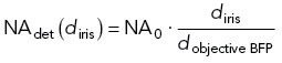
The NA of the EPI/TIRF system was changed in two ways. The first was by using different objectives: 10× 0.3 NA air, 20× 0.75 NA air, 100× 0.5–1.3 variable NA oil, 100× 1.45 NA oil, and a 100× 1.49 NA oil objective. The G-factor changed slightly depending on the objective and was corrected in each experiment. The second manner of changing the NA was used at the (conjugate) image in the back focal plane. The collar of the 100× 0.5–1.3 variable NA oil objective changes the filling of the back focal plane by opening and closing an internal iris and thereby alters the effective NA of the objective. Alternatively, the NA was changed in a conjugate image of the back focal plane that was not shared by excitation and emission. For this the emission path was relayed outside the microscope in a 4-f configuration using two 100–mm achromatic planoconvex lenses (Melles Griot). Assisted by a removable Bertrand lens (30-mm biconvex, Thorlabs), an iris was placed and aligned at the conjugate back focal plane of a 100× 1.45 NA TIRF objective. Adjusting the diameter of the iris, d_iris, changes the NA of the detection path:

7

where NA₀ is the NA of the objective and d_{objective BFP} is the diameter of the objective back focal plane. Anisotropy images were obtained and analyzed as before. The G-factor remained unaltered upon changing the collection NA.

Photobleaching in TIRF

In the same setup as described above, cells expressing the trimeric VSV-G-EGFP at the plasma membrane were photobleached in TIRF through continuous exposure to 10-mW 488-nm laser power in TIRF. Camera integration times were 100–300 ms and whole-cell basal membrane ROIs were taken, excluding large highly intense spots. Photobleaching rates were measured to be 49 ± 16 s^–1 and independent of detection NA settings.

Photobleaching in confocal

Cells expressing cytosolic EGFP-monomer or EGFP-trimer were placed on a CSU-W1 spinning disk confocal. After collimation, the excitation beam was sent through a polarization filter (MoxTek PFU04C) and a dichroic (Semrock T405/488/568/647) and via the 50-μm pinhole Nipkow spinning disk (4000 rpm) to the objective. Emission was collected with the same objective and from the dichroic was sent to two EMCCD detectors (Andor Life888) via a polarizing beam splitter (MoxTek FBF04C) and an individual filter (Chroma ET525/50m) for each camera. The polarization–extinction ratio for 488-nm excitation was 3600:1 at the back focal plane and the G-factor was 1.30±0.07. With a 100× 1.4 NA objective and 4.2 mW power at the back focal plane, the photobleaching rate of EGFP in cells was 196 ± 50 s^–1. Both polarization images were obtained simultaneously at 1 Hz with 50–150 ms integration time and both cameras were set at a measured EM gain of 140. To ensure continuous photobleaching, the laser was kept on during the photobleaching and typically reached a photobleaching fraction of 0.6–0.8 after 150–200 s. Whole-cell ROIs were used and cells containing saturated pixels were not taken further for analysis. Steady-state anisotropy single-cell analysis of cells expressing cytosolic EGFP monomer or EGFP trimer (Figure 3, A and B) were also measured on the CSU-W1 spinning disk confocal in a manner similar to that described above, with the exception of using lower laser power (0.35 mW) and longer camera exposure times (150–500 ms).

Red-edge anisotropy

Cells expressing the indicated construct were imaged on a Zeiss LSM780 with a 40× 1.2 NA water objective using highly polarized (>1500:1) 488-nm and 514-nm excitation. Excitation and emission were separated using MBS488 for 488-nm excitation or MBS458/514 for 514-nm excitation and the polarization was sequentially selected using orthogonally oriented polarizers. After identical bandpass filter settings (518–562 nm) the photon stream was detected using the 32-array GaAsP detector, which was set at pseudo photon counting mode. To ensure similar detection conditions, the power of the 514-nm excitation was increased to 162 μW as compared with 37 μW power used for 488-nm excitation and the pinhole, together with the objective collar position, was optimized before the experiment. GFP excitation under these conditions is still within the linear regime. The pixel size was set at 415 nm and the pixel dwell time at 6.3 μs and photobleaching of the sample was minimal. Due to the point scanning mode, there was a temporal difference between polarizations of 2.7 s and a wait time between two excitation conditions of 5.2 s. Switching the sequence of acquisition had no influence on the cell measurements. The G-factor of the system was determined using a 100-nM FITC solution and was 1.154 for 488-nm excitation and 1.157 for 514-nm excitation. Because the FITC chromophore is freely rotating in a solution with fast solvent dynamics, the polarization of the emission will explore all orientations, irrespective of the excitation conditions.

Theoretical calculations

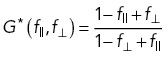
To theoretically estimate the effect of SNR at the detectors on the anisotropy measurement, a contamination was introduced into the calculation of the anisotropy,

8

with f_|| the fraction of I_|| leaking into the perpendicular channel, f_⊥ and I_⊥ the reverse. f_|| and f_⊥ are the inverses of their polarization extinction ratios. This calculation has the underlying assumption that no photons are lost during the detection. The G-factor is also affected following

9

The dynamic range using the two experimental extremes for fluorophores with aligned excitation and emission dipoles, which are r = 0 (I_|| = I_⊥) and r = 0.4 (I_|| = 3I_⊥), can now be calculated with respect to the polarization contamination.

Next, the theoretical error of the anisotropy measurement had been described by Lidke et al. (2005) and was used to calculate the relative anisotropy error dependence on both the anisotropy and the total number of photons used; see Eq. 6.

Finally, the effect of the NA of the system on the anisotropy measurement is calculated following earlier documented equations (Axelrod, 1979, 1989; Piston and Rizzo, 2008). These relate how a high-NA lens collects fluorescence emitted into three-dimensional space, (x, y, z), where the z-direction (I_z) of the sample coordinate plane is defined as the parallel (I_||) plane of the detection. Detection of dipole projections from the other directions then results in

10

11

where the normalized weighing factors, K_a,b,c, are defined following (Axelrod (1989):

12

13

14

and the angle, θ, comes from the numerical aperture, NA, via

15

where n is the refractive index. Note that for isotropic samples I_y = I_x and that for very small angles (low NA) the weighing factor K_c approaches 1, while K_a,b are close to 0. In this situation, the dipole projections in sample space (z, y) follow the detection planes (||, ⊥). For the calculations of the theoretical graphs in Figures 2D, 4C, and 6B, the anisotropy values measured with the lowest NA (mean ± σ) were used as a starting point. Note that Figure 2D has both air (n = 1) and oil (n = 1.512) objectives.

Abbreviations used:

BFP

Back focal plane

Cy3

Cyanine-3

EMCCD

electron multiplying charge coupled device

FRET

Förster’s resonance energy transfer

GPI-AP

Glycosylphosphatidylinositol-anchored proteins

LED

light emitting diode

Rho6G

rhodamine 6G

ROI

Region of interest

sCMOS

scientific complementary metal oxide semiconductor

SNR

signal to noise ratio

TIRF

total internal reflection fluorescence

VSV-G

vesicular stomatitis virus G-protein

REFERENCES

- Axelrod D (1979). Carbocyanine dye orientation in red cell membrane studied by microscopic fluorescence polarization. Biophys J 26, 557–573. [DOI] [PMC free article] [PubMed] [Google Scholar]
- Axelrod D (1989). Fluorescence Polarization Microscopy. New York, NY: Elsevier, 333–352. [PubMed] [Google Scholar]
- Bacia K, Kim SA, Schwille P (2006). Fluorescence cross-correlation spectroscopy in living cells. Nat Methods 3, 83–89. [DOI] [PubMed] [Google Scholar]
- Bader AN, Hofman EG, Voortman J, van Bergen en Henegouwen PMP, Gerritsen HC (2009). Homo-FRET imaging enables quantification of protein cluster sizes with subcellular resolution. Biophys J 97, 2613–2622. [DOI] [PMC free article] [PubMed] [Google Scholar]
- Boersma AJ, Zuhorn IS, Poolman B (2015). A sensor for quantification of macromolecular crowding in living cells. Nat Methods 12, 227–229. [DOI] [PubMed] [Google Scholar]
- Bourg N, Mayet C, Dupuis G, Barroca T, Bon P, Lécart S, Fort E, Lévêque-Fort S (2015). Direct optical nanoscopy with axially localized detection. Nat Photon 9, 587–593. [Google Scholar]
- Chattopadhyay A (2003). Exploring membrane organization and dynamics by the wavelength-selective fluorescence approach. Chem Phys Lipids 122, 3–17. [DOI] [PubMed] [Google Scholar]
- Clayton AHA, Hanley QS, Arndt-Jovin DJ, Subramaniam V, Jovin TM (2002). Dynamic fluorescence anisotropy imaging microscopy inthe frequency domain (rFLIM). Biophys J 83, 1631–1649. [DOI] [PMC free article] [PubMed] [Google Scholar]
- Cruz CAV, Shaban HA, Kress A, Bertaux N, Monneret S, Mavrakis M, Savatier J, Brasselet S (2016). Quantitative nanoscale imaging of orientational order in biological filaments by polarized superresolution microscopy. Proc Natil Acad Sci USA 113, E820–E828. [DOI] [PMC free article] [PubMed] [Google Scholar]
- Cutrale F, Rodriguez D, Hortigüela V, Chiu C-L, Otterstrom J, Mieruszynski S, Seriola A, Larrañaga E, Raya A, Lakadamyali M, et al. (2019). Using enhanced number and brightness to measure protein oligomerization dynamics in live cells. Nat Protocols 14, 616–638. [DOI] [PubMed] [Google Scholar]
- Dale RE, Eisinger J, Blumberg WE (1979). The orientation freedom of molecular probes. Biophys J 26, 161–194. [DOI] [PMC free article] [PubMed] [Google Scholar]
- Demchenko AP (2002). The red-edge effects: 30 years of exploration. Luminescence 17, 19–42. [DOI] [PubMed] [Google Scholar]
- Digman MA, Dalal R, Horwitz AF, Gratton E (2008). Mapping the number of molecules and brightness in the laser scanning microscope. Biophys J 94, 2320–2332. [DOI] [PMC free article] [PubMed] [Google Scholar]
- Ferrand A, Schleicher KD, Ehrenfeuchter N, Heusermann W, Biehlmaier O (2019). Using the NoiSee workflow to measure signal-to-noise ratios of confocal microscopes. Sci Rep 9, 1–12. [DOI] [PMC free article] [PubMed] [Google Scholar]
- Förster T (1948). Zwischenmolekulare energiewanderung un fluoreszenz. Ann Phys 6, 55–75. [Google Scholar]
- Gautier I, Tramier M, Durieux C, Coppey J, Pansu RB, Nicolas J-C, Kemnitz K, Coppey-Moisan M (2001). Homo-FRET microscopy in living cells to measure monomer–dimer transition of GFP-tagged proteins. Biophys J 80, 3000–3008. [DOI] [PMC free article] [PubMed] [Google Scholar]
- Ghosh S, Saha S, Goswami D, Bilgrami S, Mayor S (2012). Dynamic imaging of homo-FRET in live cells by fluorescence anisotropy microscopy. 505, 291–327. [DOI] [PubMed] [Google Scholar]
- Goswami D, Gowrishankar K, Bilgrami S, Ghosh S, Raghupathy R, Chadda R, Vishwakarma R, Rao M, Mayor S (2008). Nanoclusters of GPI-anchored proteins are formed by cortical actin-driven activity. Cell 135, 1085–1097. [DOI] [PMC free article] [PubMed] [Google Scholar]
- Gowrishankar K, Ghosh S, Saha S, Rumamol C, Mayor S, Rao M (2012). Active remodeling of cortical actin regulates spatiotemporal organization of cell surface molecules. Cell 149, 1353–1367. [DOI] [PubMed] [Google Scholar]
- Haldar S, Chattopadhyay A (2007). Dipolar relaxation within the protein matrix of the green fluorescent protein: a red edge excitation shift study. J Phys Chem B 111, 14436–14439. [DOI] [PubMed] [Google Scholar]
- Heckmeier PJ, Agam G, Teese MG, Hoyer M, Stehle R, Lamb DC, Langosch D (2020). Determining the stoichiometry of small protein oligomers using steady-state fluorescence anisotropy. Biophys J 119, 99–114. [DOI] [PMC free article] [PubMed] [Google Scholar]
- Hedde PN, Ranjit S, Gratton E (2015). 3D fluorescence anisotropy imaging using selective plane illumination microscopy. Opt Express 23, 22308–22310. [DOI] [PMC free article] [PubMed] [Google Scholar]
- Heintzmann R, Relich PK, Nieuwenhuizen RPJ, Lidke KA, Ried, Rieger B (2018). Calibrating photon counts from a single image. arXiv, 05654.
- Hell SW (2007). Far-field optical nanoscopy. Science 316, 1153–1158. [DOI] [PubMed] [Google Scholar]
- Hoppe A, Christensen K, Swanson JA (2002). Fluorescence resonance energy transfer-based stoichiometry in living cells. Biophys J 83, 3652–3664. [DOI] [PMC free article] [PubMed] [Google Scholar]
- Huang F, Hartwich TMP, Rivera-Molina FE, Lin Y, Duim WC, Long JJ, Uchil PD, Myers JR, Baird MA, Mothes W, et al. (2013). Video-rate nanoscopy using sCMOS camera—specific single-molecule localization algorithms. Nat Methods 10, 653–658. [DOI] [PMC free article] [PubMed] [Google Scholar]
- Jaqaman K, Loerke D, Mettlen M, Kuwata H, Grinstein S, Schmid SL, Danuser G (2008). Robust single-particle tracking in live-cell time-lapse sequences. Nat Methods 5, 695–702. [DOI] [PMC free article] [PubMed] [Google Scholar]
- Jares-Erijman EA, Jovin TM (2003). FRET imaging. Nat Biotechnol 21, 1387–1395. [DOI] [PubMed] [Google Scholar]
- Kalappurakkal JM, Anilkumar AA, Patra C, van Zanten TS, Sheetz MP, Mayor S (2019). Integrin mechano-chemical signaling generates plasma membrane nanodomains that promote cell spreading. Cell 177, 1738–1756.e23. [DOI] [PMC free article] [PubMed] [Google Scholar]
- Kampmann M, Atkinson CE, Mattheyses AL, Simon SM (2011). Mapping the orientation of nuclear pore proteins in living cells with polarized fluorescence microscopy. Nat Struct Mol Biol 18, 643–649. [DOI] [PMC free article] [PubMed] [Google Scholar]
- Kenworthy AK, Edidin MA (1998). Distribution of a glycosylphosphatidylinositol-anchored protein at the apical surface of MDCK cells examined at a resolution of <100 A using imaging fluorescence resonance energy transfer. J Cell Biol 142, 69–84. [DOI] [PMC free article] [PubMed] [Google Scholar]
- Kreis TE, Lodish HF (1986). Oligomerization is essential for transport of vesicular stomatitis viral glycoprotein to the cell surface. Cell 46, 929–937. [DOI] [PMC free article] [PubMed] [Google Scholar]
- Krishnan RV, Varma R, Mayor S (2001). Fluorescence methods to probe nanometer-scale organization of molecules in living cell membranes. J Fluoresc 11, 211–226. [Google Scholar]
- Lakowicz J (2006). Principles of fluorescence spectroscopy (3rd Ed). New York, NY: Springer Science. [Google Scholar]
- Lakowicz JR, Keating-Nakamoto S (1984). Red-edge excitation of fluorescence and dynamic properties of proteins and membranes. Biochemistry 23, 3013–3021. [DOI] [PMC free article] [PubMed] [Google Scholar]
- Lambert TJ, Waters JC (2014). Assessing camera performance for quantitative microscopy. Methods Cell Biol 123, 35–53. [DOI] [PubMed] [Google Scholar]
- Lidke D, Nagy P, Barisas B, Heintzmann R, Post J, Lidke K, Clayton A, Arndt-Jovin D, Jovin T (2003). Imaging molecular interactions in cells by dynamic and static fluorescence anisotropy (rFLIM and emFRET). Biochem Soc Transn 31, 1020–1027. [DOI] [PubMed] [Google Scholar]
- Lidke KA, Rieger B, Lidke DS, Jovin TM (2005). The role of photon statistics in fluorescence anisotropy imaging. IEEE Trans Image Process 14, 1237–1245. [DOI] [PubMed] [Google Scholar]
- Low-Nam ST, Lidke KA, Cutler PJ, Roovers RC, van Bergen en Henegouwen PMP, Wilson BS, Lidke DS (2011). ErbB1 dimerization is promoted by domain co-confinement and stabilized by ligand binding. Nat Struct Mol Biol 18, 1244–1249. [DOI] [PMC free article] [PubMed] [Google Scholar]
- Manley S, Gillette JM, Patterson GH, Shroff H, Hess HF, Betzig E, Lippincott-Schwartz J(2008). High-density mapping of single-molecule trajectories with photoactivated localization microscopy. Nat Methods 5, 155–157. [DOI] [PubMed] [Google Scholar]
- Markwardt ML, Snell NE, Guo M, Wu Y, Christensen R, Liu H, Shroff H, Rizzo MA (2018). A genetically encoded biosensor strategy for quantifying non-muscle myosin II phosphorylation dynamics in living cells and organisms. CellReports 24, 1060–1070.e4. [DOI] [PMC free article] [PubMed] [Google Scholar]
- Milo R, Phillips R (2007). Cell Biology by the Numbers, New York: Garland Science. [Google Scholar]
- Mori Y, Yoshida Y, Satoh A, Moriya H (2020). Development of an experimental method of systematically estimating protein expression limits in HEK293 cells. Sci Rep UK 10, 4798. [DOI] [PMC free article] [PubMed] [Google Scholar]
- Myšková J, Rybakova O, Brynda J, Khoroshyy P, Bondar A, Lazar J (2020). Directionality of light absorption and emission in representative fluorescent proteins. P Natl Acad Sci USA 117, 32395–32401. [DOI] [PMC free article] [PubMed] [Google Scholar]
- Nordenfelt P, et al. (2017). Direction of actin flow dictates integrin LFA-1 orientation during leukocyte migration. Nat Commun 8, 2047. [DOI] [PMC free article] [PubMed] [Google Scholar]
- Oheim M, Salomon A, Brunstein M (2020). Supercritical angle fluorescence microscopy and spectroscopy. Biophys J 118, 2339–2348. [DOI] [PMC free article] [PubMed] [Google Scholar]
- Ojha N, Rainey KH, Patterson GH (2019). Imaging of fluorescence anisotropy during photoswitching provides a simple readout for protein self-association. Nat Commun 11, 1–11. [DOI] [PMC free article] [PubMed] [Google Scholar]
- Patterson GH, Piston DW, Barisas BG (2000). Förster distances between green fluorescent protein pairs. Anal Biochem 284, 438–440. [DOI] [PubMed] [Google Scholar]
- Perrin F (1926). Polarisation de la lumière de fluorescence. Vie moyenne des molécules dans l’etat excité. J Phys Radium 7, 390–401. [Google Scholar]
- Piston DW, Kremers G-J (2007). Fluorescent protein FRET: the good, the bad and the ugly. Trends Biochem Sci 32, 407–414. [DOI] [PubMed] [Google Scholar]
- Piston DW, Rizzo MA (2008). FRET by fluorescence polarization microscopy. Methods Cell Biol 85, 415–430. [DOI] [PubMed] [Google Scholar]
- Prior IA, Muncke C, Parton RG, Hancock JF (2003). Direct visualization of Ras proteins in spatially distinct cell surface microdomains. J Cell Biol 160, 165–170. [DOI] [PMC free article] [PubMed] [Google Scholar]
- Raghupathy R, Anilkumar AA, Polley A, Singh PP, Yadav M, Johnson C, Suryawanshi S, Saikam V, Sawant SD, Panda A, et al. (2015). Transbilayer lipid interactions mediate nanoclustering of lipid-anchored proteins. Cell 161, 581–594. [DOI] [PMC free article] [PubMed] [Google Scholar]
- Rao M, Mayor S (2005). Use of Forster’s resonance energy transfer microscopy to study lipid rafts. Biochim Biophys Acta (BBA)—Mol Cell Res 1746, 221–233. [DOI] [PubMed] [Google Scholar]
- Rimoli CV, Valades-Cruz CA, Curcio V, Mavrakis M, Brasselet S (2022). 4polar-STORM polarized super-resolution imaging of actin filament organization in cells. Nat Commun 13, 301. [DOI] [PMC free article] [PubMed] [Google Scholar]
- Rizzo MA, Piston DW (2005). High-contrast imaging of fluorescent protein FRET by fluorescence polarization microscopy. Biophys J 88, L14–L16. [DOI] [PMC free article] [PubMed] [Google Scholar]
- Rizzo MA, Springer G, Segawa K, Zipfel WR, Piston DW (2006). Optimization of pairings and detection conditions for measurement of FRET between cyan and yellow fluorescent proteins. Microsc Microanal 12, 238–254. [DOI] [PubMed] [Google Scholar]
- Sergé A, Bertaux N, Rigneault H, Marguet D (2008). Dynamic multiple-target tracing to probe spatiotemporal cartography of cell membranes. Nat Methods 5, 687–694. [DOI] [PubMed] [Google Scholar]
- Sharma P, Varma R, Sarasij RC, Ira, Gousset K, Krishnamoorthy G, Rao M, Mayor S (2004). Nanoscale organization of multiple GPI-anchored proteins in living cell membranes. Cell 116, 577–589. [DOI] [PubMed] [Google Scholar]
- Squire A, Verveer PJ, Rocks O, Bastiaens PIH (2004). Red-edge anisotropy microscopy enables dynamic imaging of homo-FRET between green fluorescent proteins in cells. J Struct Biol 147, 62–69. [DOI] [PubMed] [Google Scholar]
- Strickler SJ, Berg RA (1962). Relationship between absorption intensity and fluorescence lifetime of molecules. J Chem Phys 37, 814–822. [Google Scholar]
- Stryer L (1978). Fluorescence energy transfer as a spectroscopic ruler. Annu Rev Biochem 47, 819–846. [DOI] [PubMed] [Google Scholar]
- Suhling K, Siegel J, Phillips D, French PMW, Lévêque-Fort S, Webb SED, Davis DM (2002). Imaging the environment of green fluorescent protein. Biophys J 83, 3589–3595. [DOI] [PMC free article] [PubMed] [Google Scholar]
- Tramier M, Piolot T, Gautier I, Mignotte V, Coppey J, Kemnitz K, Durieux C, Coppey-Moisan M (2003). Homo-FRET versus hetero-FRET to probe homodimers in living cells. Methods Enzymol 360, 580–597. [DOI] [PubMed] [Google Scholar]
- van den Berg J, Boersma AJ, Poolman B (2017). Microorganisms maintain crowding homeostasis. Nat Rev Microbiol 15, 309–318. [DOI] [PubMed] [Google Scholar]
- Varma R, Mayor S (1998). GPI-anchored proteins are organized in submicron domains at the cell surface. Nature 394, 798–801. [DOI] [PubMed] [Google Scholar]
- Vliet LJ, Sudar D, Young IT (1998). Digital Fluorescence Imaging Using Cooled CCD Array Cameras. In: Cell Biology: A Laboratory Handbook. ed. Celis JE, New York, NY: Academic Press, 109–120. [Google Scholar]
- Volkmer A, Subramaniam V, Birch DJS, Jovin TM (2000). One- and two-photon excited fluorescence lifetimes and anisotropy decays of green fluorescent proteins. Biophys J 78, 1589–1598. [DOI] [PMC free article] [PubMed] [Google Scholar]
- Wallrabe H, Periasamy A (2005). Imaging protein molecules using FRET and FLIM microscopy. Curr Opin Biotech 16, 19–27. [DOI] [PubMed] [Google Scholar]
- Weber G (1954). Dependence of the polarization of the fluorescence on the concentration. Trans Faraday Soc 50, 552–554. [Google Scholar]
- van Zanten TS, Cambi A, Koopman M, Joosten B, Figdor CG, Garcia-Parajo MF (2009). Hotspots of GPI-anchored proteins and integrin nanoclusters function as nucleation sites for cell adhesion. Proc Natl Acad Sci 106, 18557–18562. [DOI] [PMC free article] [PubMed] [Google Scholar]
- van Zanten TS, Mayor S (2015). Current approaches to studying membrane organization. F1000research 4, F1000 Faculty Rev-1380. [DOI] [PMC free article] [PubMed] [Google Scholar]
- Zhang Q, Zhong L, Tang P, Yuan Y, Liu S, Tian J, Lu X (2017). Quantitative refractive index distribution of single cell by combining phase-shifting interferometry and AFM imaging. Sci Rep UK 7, 2532. [DOI] [PMC free article] [PubMed] [Google Scholar]
Associated Data
This section collects any data citations, data availability statements, or supplementary materials included in this article.