Cell cycle oscillations driven by two interlinked bistable switches

Abstract

Regular transitions between interphase and mitosis during the cell cycle are driven by changes in the activity of the enzymatic protein complex cyclin B with cyclin-dependent kinase 1 (Cdk1). At the most basic level, this cell cycle oscillator is driven by negative feedback: active cyclin B-Cdk1 activates the anaphase-promoting complex/cyclosome, which triggers the degradation of cyclin B. Such cell cycle oscillations occur fast and periodically in the early embryos of the frog Xenopus laevis, where several positive-feedback loops leading to bistable switches in parts of the regulatory network have been experimentally identified. Here, we build cell cycle oscillator models to show how single and multiple bistable switches in parts of the underlying regulatory network change the properties of the oscillations and how they can confer robustness to the oscillator. We present a detailed bifurcation analysis of these models.

INTRODUCTION

Biological systems are often characterized by periodic behavior, ranging from the circadian clock to the cell division cycle and our heart rate. These biological rhythms are all generated by biochemical clock-like oscillators (Goldbeter and Berridge, 1996; Novák and Tyson, 2008; Ferrell et al., 2011; Winfree, 2011; Beta and Kruse, 2017; Mofatteh et al., 2021). In the case of our heart rate, the sinoatrial node generates 50–150 action potentials per minute, depending on the oxygen demands of the body. Similarly, the period of the cell division cycle ranges from 10 to 30 min in rapidly cleaving early embryos to about 10–30 h in dividing somatic cells. However, despite the large variation in the period of these oscillations, the amplitude remains reasonably unchanged. This has been attributed to the presence of positive feedback in the regulatory network of the biological oscillator (Tsai et al., 2008). While any (biological) oscillator requires negative feedback to reset the system after each cycle (Thomas, 1981), positive feedback has been shown to be important to generate robust, large-amplitude oscillations with tunable frequency (Brandman et al., 2005; Tsai et al., 2008). At the core of such relaxation oscillations is the fact that positive feedback can generate bistability in part of the regulatory network. Additional negative feedback can then drive oscillations along both branches of the bistable response curve. As a result, such relaxation oscillators exist over a wider range of parameters and allow the system to regulate its oscillation frequency without compromising its amplitude. Without a built-in bistable switch, changes in the frequency would strongly correlate with changes in the amplitude.

In the early embryo of the frog Xenopus laevis, it has been shown experimentally and theoretically that cell cycle oscillations are driven by a positive-plus-negative-feedback network. There exists a (time-delayed) negative-feedback loop between active enzymatic protein complexes of cyclin B with cyclin-dependent kinase 1 (Cdk1) and the anaphase-promoting complex/cyclosome (APC/C), which triggers the degradation of cyclin B (Yang and Ferrell, 2013; Rombouts et al., 2018). Positive feedback exists in the regulation of the activity of the Cdk1 complexes by the enzymes Wee1, Myt1. and Cdc25, which leads to bistability of Cdk1 activity in function of cyclin B concentration (Pomerening et al., 2003; Sha et al., 2003) (see Figure 1, a and c). However, measurements also show that the bistability in the dose-response curve of cyclin B versus active cyclin B-Cdk1 is essentially abolished after the first cell cycle (Tsai et al., 2014). Despite this loss of bistability, cell cycle oscillations persist and at a faster pace. Interestingly, various new experiments point toward the existence of a second bistable switch in the system, one where APC/C gets activated in a bistable manner by active Cdk1 (Mochida et al., 2016; Rata et al., 2018; Kamenz et al., 2021) (see Figure 1b). This bistable switch is related to the feedback loops involving Greatwall (Gwl), ENSA-Arpp19, and PP2A:B55 (see Figure 1d). This triggers the question of what the advantage might be of interlinking bistable switches to generate cell cycle oscillations when combined with negative feedback. We recently found that having multiple bistable switches can increase the parameter range of oscillations while also allowing switches between regions of qualitatively different oscillations (in terms of period and amplitude) (De Boeck et al., 2021). Having multiple positive-feedback loops (which can lead to bistability) has been shown to allow for improving speed and resistance to noise (Brandman et al., 2005), which could also indicate a potential advantage of interlinked bistable switches. Moreover, the cell cycle has also been studied as a chain of interlinked bistable switches, which can increase the robustness of cell cycle transitions (Hutter et al., 2017; Novák and Tyson, 2021). However, as far as we know, no study has looked in detail at how multiple bistable switches affect the dynamic properties of a resulting biological oscillator.

FIGURE 1:

Experimentally measured bistable dose-response curves (a and b), their corresponding cell cycle regulatory networks (c and d), and their approximations using Eq. (5) in e and f, respectively. (a) Experimentally measured Cdk1 activity (a.u.) in function of cyclin B concentration (nM) (Pomerening et al., 2003). (e) Approximated response curve using (b,C_x,C_y) = (1.88, 55 nM, 0.5) as parameters. (b) Experimentally measured APC/C activity (a.u.) in function of active cyclin B-Cdk1 (nM) (Kamenz et al., 2021). (f) Approximated response curve using (b,C_x,C_y) = (1.95,20 nM, 0.5) as parameters.

Here, we theoretically investigate how oscillations emerge by combining negative feedback with one or multiple interlinked bistable switches. We consider only deterministic systems and do not explicitly implement the various molecular interactions that lead to the different bistable switches (those have been studied elsewhere; e.g., see Novak and Tyson, 1993; Pomerening et al., 2003; Sha et al., 2003; Mochida et al., 2016; Rata et al., 2018; De Boeck et al., 2021; Kamenz et al., 2021). Instead, we approximate each experimentally measured bistable response curve by using a single cubic function (see Figure 1, e and f). We then use them to study how oscillations arise from negative feedback in combination with one or two such bistable switches of various shapes. In doing so, we show that having two interlinked bistable switches leads to oscillations over a wider range of parameters, thus increasing their robustness.

RESULTS

A generic cell cycle oscillator model based on experimentally measured bistable response curves

Approximating bistable response curves.

We choose a cubic function x = f(y) = y – by² + y³ as one of the simplest functions to describe an S-shaped curve. The turning points (folds F₁ and F₂) of this S-shaped response curve can be found by solving df(y)/dy = 0:

1

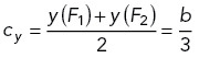
which shows that the system becomes S-shaped when b = _√3, and the center C = (c_x,c_y) of the S-shaped region is given by

2

3

The whole S-shaped region (going from F₁ to F₂) thus scales with b. To approximate experimentally measured dose-response curves, we introduce the transformation (x,y) = (c_xX/C_x,c_yY/C_y), thus repositioning the center of the S-shaped curve from (x,y) = (c_x,c_y) to the point (X,Y) = (C_x,C_y). In Figure 2a, such response curves are plotted for various values of b using C_x = 50 and C_y = 0.5. In this case the left fold F₁ touches the y-axis (x = 0) when b = 2. Figure 2b shows the same response curves, but now multiplied by X. The reasoning is that, in the context of cell cycle regulation, the red response curves in Figure 2a could be used to approximate the fraction (from 0 to 1) of active Cdk1 (or APC/C) in function of cyclin B (or active Cdk1), while the response curve in Figure 2b could be interpreted as the total amount of active Cdk1 in function of cyclin B levels. The blue curves are thus the red ones multiplied by the amount of cyclin B, where we use the realistic assumption that all cyclin B proteins quickly bind to Cdk1 to form a complex.

FIGURE 2:

(a) Input (X)–output (Y) response curves given by Eq. (5) with C_x = 50 and C_y = 0.5 for increasing bistability by increasing the parameter b. (b) The same response curves as in a, but now the output Y is multiplied by the input X.

Figure 1, a and b, shows experimentally measured bistable dose-response curves, where the blue markers indicate the measured values when increasing the input, while the red markers depict the measurements when subsequently decreasing the input again. Pomerening et al. (2003) controlled the concentration of (nondegradable) cyclin B in frog egg extracts and then proceeded to measure the activity of cyclin B-Cdk1 complexes (Figure 1a). This approach allowed the authors to reveal the presence of hysteresis in the system, where for cyclin B concentrations between approximately 40 and 70 nM the system could be in two possible steady states: low Cdk1 activity (corresponding to interphase) or high Cdk1 activity (corresponding to mitotic phase). Similar experiments were carried out by Sha et al. (2003) around the same time. We chose (b,C_x,C_y) = (1.88, 55 nM, 0.5) by hand to visually approximate the experimentally measured curve (Figure 1e). While this approximation by the cubic expression is not able to capture the finer details of the measured response curve, it allows description of the region of bistability. More recently, Kamenz et al. (2021) used similar techniques in frog egg extracts to measure the activity of APC/C by quantifying how quickly fluorescently labeled securin was degraded by the proteasome (triggered by APC/C through ubiquitination) in the presence of various levels of active Cdk1 complexes. These experiments once again revealed bistability of APC/C activity in function of Cdk1 activity (Figure 1b). Similarly as before, using (b,C_x,C_y) = (1.95, 20 nM, 0.5), we obtain a good approximation of this response curve (Figure 1f).

To turn the S-shaped dose-response curves in Figure 2 into a dynamical bistable system, we introduce the following ordinary differential equation (ODE), which ensures that the system will approach the steady state solutions given by the cubic function, and a parameter ϵ that controls how fast the system will relax to the steady state solution:

4

or when repositioned to the point (X,Y) = (C_x,C_y) as depicted in Figures 1 and 2, the ODE becomes the following:

5

Note that in this work sometimes we use the terms “bistable” and “S-shaped” interchangeably for ease of notation. However, we want to emphasize that strictly speaking having an S-shaped dose-response curve does not imply that the overall dynamical system behaves in a bistable way. Dynamical system (4) does exhibit bistability for a range of input values x, but this depends on the details of the dynamical system built on such S-shaped response curves. In particular, we will often refer to combining “bistable” response curves to study oscillator properties. In such a case, we refer to the fact that a small part of the interaction network can function in a bistable manner in the absence of negative feedback, but the system as a whole behaves as an oscillator when adding negative feedback through APC/C-mediated cyclin B degradation.

Turning bistable response curves into a dynamical cell cycle oscillator model

How can we now use such equations that capture bistability in different parts of the cell cycle regulatory network to create a model of cell cycle oscillations? First, we introduce an ODE to describe the synthesis and degradation of cyclin B (X); see Eq. (6). Cyclin B is synthesized at a constant rate (k_s [nM/min]), where this synthesis rate is experimentally known to be around 1 nM/min (see Table 1 and Chang and Ferrell, 2013; Yang and Ferrell, 2013). Furthermore, it is degraded at a fixed basal level (d₁ [min⁻¹]), as well as in a APC/C (Z)–dependent manner (d₂ [min⁻¹]). Here, experiments have motivated the APC/C-driven degradation rate d₂ to be approximately in the range 0.05–0.5 min⁻¹ (Yang and Ferrell, 2013; Rombouts et al., 2018) and d₁ should be much smaller (exact value of d₁ not critical for the dynamics discussed in this work). Second, in Eq. (7) we capture the experimental observation of bistability in Cdk1 activity in response to fixed values of cyclin B concentration; see Figure 1, a, c, and e. X corresponds to cyclin B concentration, and Y is the fraction of active Cdk1 complexes. For fixed values of cyclin B concentration (X), the system relaxes to the steady state solution shown in Figure 1e. Third, in Eq. (8) APC/C activity (Z) is controlled by Cdk1 activity (X × Y). So, the variables are defined as follows:

• X = cyclin B concentration (nM),

• Y = fraction of active Cdk1 complexes (a.u.),

• X × Y = concentration of active cyclin B-Cdk1 complexes (nM), Z = APC/C activity (a.u.).

TABLE 1:

Parameters used in the different cell cycle oscillator models: built on cyclin B (X)-Cdk1 (XY) bistability (13–14), built on Cdk1 (XY)-APC/C (Z) bistability (15–16), and built on the two interlinked bistable switches (6–8).

Parameter	Meaning	(13)–(14)	(15)–(16)	(6)–(8)	Reference
ks	Cyclin synthesis rate	1 nM/min	2.3 nM/min	1 nM/min	Chang and Ferrell (2013)
d 1	Basal degradation rate	0.001 min−1	0.001 min−1	0.001 min−1	Chang and Ferrell (2013)
d 2	APC/C-driven degradation rate	0.1 min−1	0.1 min−1	0.05 min−1	Rombouts et al. (2018)
by	Controls bistability range	1.88	–	1.88	Pomerening et al. (2003)
bz	Controls bistability range	–	1.9	1.95	Kamenz et al. (2021)
ϵy	Relaxation time	0.02 min	–	0.02 min	This work
ϵz	Relaxation time	–	0.02 min	0.1 min	This work
n	Hill exponent	20	–	–	Yang and Ferrell (2013)
Cx	Location switch in X	55 nM	–	55 nM	Pomerening et al. (2003)
Cy	Location switch in Y	0.50	–	0.50	Pomerening et al. (2003)
Cxy	Location switch in XY	27 nM	50 nM	20 nM	Kamenz et al. (2021)
Cz	Location switch in Z	–	0.50	0.50	Kamenz et al. (2021)

Their dynamical evolution is controlled by this set of ODEs:

6

7

8

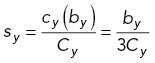
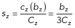
using the following scaling factors s_x, s_y, s_z, s_xy:

9

10

11

12

Using the system parameters given in Table 1, we find oscillations in (X, Y, Z) driving the cell cycle forward. In Figure 3, we modulate the parameter b_y in time from 1.94 to 1.73 to 1.91, mimicking the experimental observation that the S-shaped response curve of Cdk1 activity in function of cyclin B concentration is abolished after the first embryonic cell cycle (Tsai et al., 2014). As a result, the first cell cycle is long (approximately 75 min), while the next cell cycles are short (approximately 30 min). Finally, after approximately 10 cell cycles, embryonic divisions gradually slow down again, which has been attributed at least partially to increases in b_y (the ratio of enzymatic activity of Wee1 vs. Cdc25 increases). The experimental data of embryonic cell division timing at 21–23°C plotted (in red) in Figure 3c are taken from Satoh (1977) (with the data of the first cell cycle; our own unpublished data). Figure 3 thus shows that tuning the width of the underlying bistable response curves permits changing the experimentally observed changes in period of the cell cycle oscillator. While most parameters in Table 1 are experimentally well motivated, the timescale parameters ϵ_y and ϵ_z are less well known and getting the results in Figure 3 required ϵ_y and ϵ_z to be sufficiently small. ϵ_y is mainly determined by the phosphorylation and dephosphorylation rates of Cdk1 by Wee1 and Cdc25 (and vice versa). The absolute values of these rates are experimentally not well known (see discussion in Yang and Ferrell, 2013). The other timescale determining the activation of APC/C by Cdk1 is given by ϵ_z and has been measured to be time-delayed (with a delay time of minutes) (Yang and Ferrell, 2013; Rombouts et al., 2018). To choose values for (ϵ_y, ϵ_z), we carried out simulations over a wide range of parameters, analyzing the resulting cell cycle oscillation period for each parameter set. In doing so, we found that ϵ_y needs to be smaller than approximately 10⁻², while ϵ_z needs to be smaller than approximately 10⁻¹ to obtain realistic oscillation periods. Having sufficiently small values of ϵ_y and ϵ_z (see Table 1) also allows for a clear interpretation of the dynamics as relaxation-like oscillations.

FIGURE 3:

(a) Simulation of the model for the cell cycle oscillator built on two interlinked bistable switches. (b) In time b_y was changed from 1.94 to 1.73 to 1.91. (c) The detected period for every consecutive cell cycle: in black for the simulated time series in a, and in red for the experimentally measured periods (mean period ± one SD) (Satoh, 1977; Anderson et al., 2017).

In what follows, we will introduce and elaborately study the dynamics of different oscillator models built on each of the bistable switches in Figure 1, as well as both switches combined. Note that we introduced a similar approach in De Boeck et al. (2021), which allowed for greater control over the response curve. However, here we limit ourselves to a cubic nonlinear function as it is likely one of the simplest expressions that can be used to reproduce a bistable switch.

A cell cycle oscillator built on cyclin B-Cdk1 bistability

A cell cycle oscillator model can be constructed by taking into account the experimental observation of bistability in Cdk1 activity in response to fixed values of cyclin B concentration; see Figure 1, a, c, and e. To do so, we study a simplified version of Eqs. (6)–(8). We complement Eq. (7) with a modified version of Eq. (6), assuming that APC/C activity (Z) is a nonlinear, ultrasensitive function of Cdk1 activity as measured in Yang and Ferrell (2013) and Tsai et al. (2014):

13

14

The parameters are given in Table 1, where additionally the scaling factors s_x and s_y are given by Eqs. (9)–(12). Using the parameters from Table 1, Figure 4a shows the time evolution of cyclin B concentration (X) in blue and the corresponding concentration of active Cdk1 (X × Y) in orange. This simple model thus reproduces cell cycle oscillations with a realistic period of around 30 min, where Cdk1 is periodically sharply activated and inactivated.

FIGURE 4:

Simulation of the model for the cell cycle oscillator built on cyclin B-Cdk1 bistability [see Eqs. (13)–(14)]. Time series (a and e) and phase space (b and f). Phase diagram in b_y and C_xy (c and g) showing the period of the oscillation in blue color map, the Hopf bifurcations (blue line), and the intersection of the cyclin B-nullcline with the folds of the cyclin B-Cdk1-nullcline (orange line). Bifurcation diagram in C_xy (d and h) for b_y =1.88 showing the value of active cyclin B-Cdk1 of the stationary state (in red) and the maximum of the oscillation (in blue). The Hopf bifurcations are indicated by H_1,2 and the fold of cycles by FC.

The functioning of this oscillator can be visually interpreted in the phase space (X, X × Y) = (cyclin B, active Cdk1) by looking at the nullclines (curves where dX/dt = 0 or dY/dt = 0) in Figure 4b. The Cdk1 (Y)-nullcline (dY/dt = 0) in orange shows the typical S-shaped curve, and the cyclin B (X)-nullcline (dX/dt = 0) in blue illustrates the ultrasensitive activation of APC/C when Cdk1 activity crossed the threshold C_xy = 27 nM. The cell cycle oscillations plotted in Figure 4a correspond to a limit cycle attractor in this phase space, plotted in gray in Figure 4b. The oscillations consist of four phases [indicated as (1)–(4)]:

1. Cyclin B is synthesized at a rate k_s, while APC/C is inactive, and the system moves along the bottom branch of the S-shaped curve;

2. The system reaches the turning point of the S-shaped curve, at which point Cdk1 is quickly (if ϵ_y is sufficiently small) activated and the system jumps to the top branch of the S-shaped curve;

3. Active Cdk1 activates APC/C, cyclin B is degraded at a rate dominated by d₂, such that the system moves down along the top branch of the S-shaped curve;

4. Finally, the left turning point of the S-shaped curve is reached and the system jumps down to the bottom branch again, thus inactivating APC/C such that the system is reset and phase 1 starts over.

Notice that the blue cyclin B-nullcline intersects the middle branch of the orange S-shaped Cdk1-nullcline. For small values of ϵ_y, this serves as a condition for obtaining relaxation-type oscillations in the system. This visual interpretation allows us to easily see when cell cycle oscillations exist in this model. For example, by changing the APC/C activation threshold C_xy the cyclin B-nullcline can be shifted up or down. When C_xy is changed outside of the approximate interval [22 nM, 32 nM] (the gray region in Figure 4b), it will intersect the top or bottom branch of the S-shaped nullcline, leading to a stable steady state solution. This can also be seen in Figure 4c, where we show the region of oscillations (and their period) in the parameter space (b_y,C_xy). Here, the orange lines indicate the parameter values for which the cyclin B-nullcline intersects either turning point of the S-shaped Cdk1-nullcline. As expected, cell cycle oscillations that encircle the S-shaped Cdk1-nullcline have a higher amplitude and period, and they are contained between these orange lines in the parameter space.

When increasing the width of the S-shaped Cdk1-nullcline further (by increasing b_y), the oscillation period increases and the parameter region of oscillations decreases. This makes sense as it becomes increasingly difficult for the cyclin B-nullcline to intersect the middle branch of the S-shaped nullcline. Relaxation oscillations of higher amplitude and period disappear entirely above b_y ≈ 1.93, when both turning points of the S-shaped nullcline have the same y-value: X(F₁) × Y (F₁) = X(F₂) × Y (F₂). Note that there still exists a narrow region of fast, small-amplitude oscillations above this critical point. These oscillations correspond to a limit cycle that does not encircle the top and bottom branch of the S-shaped nullcline.

From a dynamical systems perspective, the cell cycle oscillations originate from a Hopf bifurcation. When constructing a bifurcation diagram for changing values of the APC/C activation threshold (C_xy), we find that the steady state solutions (in red) lose their stability at two Hopf bifurcations, H₁ and H₂ (see Figure 4, c and d). The maxima of the resulting oscillations are plotted in blue. Considering that Cdk1 activity is low when the steady state solution lies on the lower branch of the bistable switch and Cdk1 activity is high when on the upper branch, the low-activity steady state loses its stability in a supercritical bifurcation (H₁), while the high-activity steady state solution stabilizes in a subcritical bifurcation (H₂) when increasing the APC/C activation threshold (C_xy). Beyond H₁, the oscillations are initially of low amplitude and period (region I) but then sharply increase in amplitude and period when increasing C_xy (region II). Such sharp transitions are referred to as Canard behavior, or Canard explosion, typical in fast–slow systems (Desroches et al., 2012; Kuehn, 2015). As H₂ is a subcritical bifurcation, there exists a (narrow) region in parameter space (between H₂ and a fold of cycles FC; region III) where stable oscillations coexist with a stable high-activity steady state solution.

How do the cell cycle oscillations change when keeping the nullclines fixed but changing the relaxation time ϵ_y and the rates of cyclin synthesis k_s and APC/C-driven degradation d₂? The visual interpretation using the location of intersecting nullclines as a way to predict the presence of cell cycle oscillations requires sufficient timescale separation. When ϵ_y increases (i.e., the system is no more on the singular perturbation regime), this is no longer valid. In this limit, the Canard explosion can be defined in terms limit cycle’s curvature change and detected using the inflection-line method (Brøns and Bar-Eli, 1994; Desroches and Jeffrey, 2011).

In Figure 4, e–h, we repeat the same analysis as in Figure 4, a–d, but now for ϵ_y = 0.2 min, where the oscillations are less relaxation-like and thus more sinusoidal (Figure 4, e and f). Here, oscillations overall exist in a smaller region in parameter space, but they do persist beyond b_y ≈ 1.93, which was a critical point when the timescale separation was sufficiently large (Figure 4g). When increasing ϵ_y even further, oscillations are lost for these parameters, even though the cyclin B-nullcline still intersects the middle branch.

In Figure 5, we illustrate how the rates of cyclin synthesis k_s and APC/C-driven degradation d₂ affect the cell cycle oscillations. As the synthesis and degradation rates increase, the period of the oscillations decreases (Figure 5a). Furthermore, oscillations exist only within a well-defined region of synthesis and degradation rates. For a realistic value of the degradation rate (d₂ = 0.1 min⁻¹), Figure 5b illustrates in more detail how the oscillations change with the cyclin synthesis rate k_s. At high k_s, oscillations originate in a Hopf bifurcation (H₁) that shows a fast Canard increase in period and amplitude (see inset). For lower values of k_s the oscillations disappear in a homoclinic bifurcation (indicated by the black dots). The oscillation period increases (in principle toward ∞) when approaching the homoclinic bifurcation (Hom). For larger values of the degradation rate d₂, the oscillations become more sinusoidal, faster, and of lower amplitude. Here, for low synthesis rates k_s, stable oscillations are born in a supercritical Hopf bifurcation H₂ (see Figure 5c). The oscillations are then lost at higher values of the synthesis rate k_s in either a fold of cycles (FC) where the stable limit cycle touches the unstable limit cycle born in a subcritical Hopf bifurcation H₃ (see Figure 5c for d₂ = 1 min⁻¹ and for d₂ = 1.8 min⁻¹) or in another supercritical Hopf bifurcation H₃ (see Figure 5c for d₂ = 4 min⁻¹). Note that the Canard cycles that originate at the Canard explosion shown in Figure 5c for d₂ = 1 min⁻¹ may persist when decreasing d₂ (see Figure 5b for d₂ = 0.1 min⁻¹), leading to a homoclinic connection with a Canard segment. The Hopf and saddle-node bifurcations, as well as the FCs, are plotted in Figure 5a, where the oscillations are bounded by the supercritical Hopf bifurcations, the FC, and/or the homoclinic bifurcations (the homoclinic bifurcation line is unpublished). Overall, the dynamics unfold from two Takens–Bogdanov (TB) points of codimension-two (in purple). Here, the saddle-node bifurcation, Hopf bifurcation, and homoclinic bifurcations come together, while the FC also occurs very close to it.

FIGURE 5:

(a) Phase diagram of model (13)–(14) in the parameter space (k_s,d₂). Different bifurcations are indicated: Hopf bifurcations (H₁, H₂, H₃-blue), folds of cycles (FC–green), and saddle-node bifurcations (SN₁, SN₂–red). TB₁, TB₂ are two codimension-two Takens–Bogdanov points. When stable oscillations exist, their period is also indicated in a blue color scale. (b, c) Bifurcation diagrams in function of cyclin synthesis k_s for different values of the degradation rate d₂. All other parameters are given in Table 1.

A cell cycle oscillator built on Cdk1-APC/C bistability

A recent series of experiments (Mochida et al., 2016; Rata et al., 2018; Kamenz et al., 2021) demonstrated that there also exist bistable response functions elsewhere in the cell cycle regulatory network, that is, in the central regulation of APC/C activity by active Cdk1 (see Figure 1b). Starting from Eqs. (6)–(8), we omit Eq. (7) by assuming that cyclin B quickly binds to Cdk1 and that each such cyclin B-Cdk1 complex is in its active state (Y = 1) and X × Y = X. We then choose a parameter set (see Table 1) to approximate this experimentally measured response curve of APC/C activity (Z) in function of the concentration of active Cdk1 (X × Y); see Figure 1f. This leaves us with the following dynamical cell cycle control system:

15

16

The control parameters are given in Table 1. Note that the parameters to describe the bistable response curve are different from the ones found to fit the experimentally measured curve in Figure 1f. To obtain oscillations in this model, the parameters need to be different to compensate for the absence of the (cyclin B, active Cdk1) switch, as can be observed in phase diagrams shown in Figures 6c and 7a.

FIGURE 6:

(a) Simulation of model (15)–(16) for the cell cycle oscillator built on Cdk1-APC/C bistability: time series (a) and phase space (b). (c) (b_z,C_xy)-phase diagram with Hopf bifurcations in blue. Parameters are given in Table 1.

FIGURE 7:

(a) Phase diagram of model (15)–(16) in the parameter space (k_s,d₂). Different bifurcations are indicated: Hopf bifurcations (H₁–blue), fold of cycles (FC–green), and saddle-node bifurcations (SN₁, SN₂–red). TB₁, TB₂ and TB₃ are three codimension two Takens–Bogdanov points. When stable oscillations exist, their period is also indicated in a blue color scale. (b) Bifurcation diagrams in function of cyclin synthesis k_s for d₂ = 0.1,1, and 5 min⁻¹. All other parameters are given in Table 1.

Oscillations in the activity of Cdk1 and APC/C are shown in Figure 6a. While the oscillations look very similar to the ones in Figure 4, a and b, there are important differences. The oscillations are also relaxation-like, but here it is not Cdk1 (blue) that is periodically sharply activated and deactivated, but rather the activity of APC/C (green). Indeed, it is now the APC/C-nullcline (dZ/dt = 0) that is S-shaped in the phase space (X × Y, Z) = (active Cdk1, active APC/C), in contrast to model (13)–(14), where active Cdk1 was an S-shaped function of cyclin B. Another difference is that the cyclin nullcline (dX/dt = 0) is no longer ultrasensitive [as in model (13)–(14)]. Despite these differences, the origin of oscillations can be similarly interpreted in the phase space in Figure 6b. Oscillations exist when the cyclin nullcline (blue) intersects the middle branch of the S-shaped APC/C-nullcline (green), provided that the relaxation time ϵ_z is sufficiently small, ensuring that APC/C is quickly activated/deactivated.

Similar as in the preceding section, the oscillations originate from a Hopf bifurcation, shown by the blue line in Figure 6c, illustrating how the nonlinearity b_z (controlling the width of the S-shaped APC/C response curve) and C_xy (controlling the threshold of APC/C activation) affect the region of oscillations. Although the S-shaped response curve relates to different variables in models (13)–(14) and (15)–(16), the two show similar dynamical properties. Figure 7a shows the region of oscillations when changing the cyclin synthesis rate k_s and degradation rate d₂. Representative bifurcation diagrams for different values of d₂ are plotted in Figure 7b. An unstable limit cycle is created in a subcritical Hopf bifurcation (H₁), which is stabilized in a FC. These limit cycle oscillations disappear at larger k_s in a homoclinic bifurcation (Hom). Several such homoclinic bifurcations, as well as a FC and another Hopf bifurcation H₂, occur close to the saddle-node bifurcation SN₂. A more detailed bifurcation analysis of this complicated scenario is left for future work. The main Hopf bifurcation and saddle-node bifurcation lines are shown in Figure 7a in the (k_s, d₂) parameter plane, illustrating that the dynamics again unfold from several codimension two TB points.

A cell cycle oscillator built on two interlinked bistable switches

Next, we wondered what would happen if we consider the full model (6)–(8) that incorporates both S-shaped responses present in models (13)–(14) and (15)–(16) that we studied separately in the two preceding sections. Using the parameters given in Table 1, which are based on experimentally measured S-shaped response curves (Figure 1), we simulated the dynamics of model (6)–(8). Figure 8a shows the resulting oscillations in cyclin B concentration (blue), concentration of active Cdk1 (orange), and APC/C activity (green). A first observation is that the oscillations are again relaxation-like as not only is cyclin B-Cdk1 periodically sharply (de)activated (with a relaxation time ϵ_y), but also APC/C activity has a similar sharp transition (with a relaxation time ϵ_z). The cell cycle model (6)–(8) consists of three ODEs. Therefore, it is no longer possible to interpret all of its dynamics in a two-dimensional (2D) phase plane. It is, however, still informative to project the nullclines and the three-dimensional system dynamics in the phase plane (X, X × Y) = (cyclin B, active Cdk1) and in the plane (X × Y, Z) = (active Cdk1, active APC/C). This can be seen in Figure 8, b and c, respectively, which reveals both bistable switches that were measured experimentally (Figure 1) as nullclines: the (cyclin B, active Cdk1) switch (in orange, the Cdk1-nullcline: dY /dt = 0) and the (active Cdk1, active APC/C) switch (in green, the APC/C-nullcline: dZ/dt = 0). The third nullcline (in blue, the cyclin B-nullcline: dX/dt = 0) requires using the expression of either the APC/C-nullcline or the Cdk1-nullcline as well being able to plot it in the chosen 2D phase planes, which is why we label them as accordingly. The gray lines indicate the projected limit cycle trajectory in the respective phase planes. This reveals that the oscillations are mainly driven by the (cyclin B, active Cdk1) switch (in orange) as the limit cycle closely circles around this switch. This results in oscillations of large amplitude in Cdk1 activity, as Cdk1 is activated [to a value of Cdk1(F₂(Cdk1))] when crossing the fold of the Cdk1-nullcline [F₂(Cdk1)]. As this Cdk1 activity is much larger than the right fold of the APC/C-nullcline [F₂(APC)], APC/C is strongly activated, leading to cyclin B degradation and deactivation of both Cdk1 and APC/C, thus resetting the cell cycle oscillator. We can again observe that the different projected nullclines cut each other in the middle branch of each switch. Whereas in our previous two-oscillator model this was found to be a good indicator for oscillations, we remark that this should not necessarily be the case here as the system is no longer 2D.

FIGURE 8:

Simulation of the model for the cell cycle oscillator built on two interlinked bistable switches: time series (a) and phase space projections (b and c). Parameters are as in Table 1.

We then again explored the influence of the rates of synthesis (k_s) and degradation of cyclin B (d₂); see Figure 9. The presence of two bistable switches makes the bifurcation diagrams more complex, now introducing additional saddle-node and Hopf bifurcations. Despite the increased complexity, overall the response when increasing the synthesis rate is similar. Let us more closely consider our standard case from Table 1 where d₂ = 0.05 min⁻¹; see the last panel in Figure 9b and the phase space projections for selected values of k_s in Figure 9c. For low synthesis rates (e.g., k_s = 0.3 nM/min), the system finds itself in a state of low Cdk1 and APC/C activity. When increasing k_s to about 0.45, the system starts to oscillate at the Hopf bifurcation H₁. The onset of oscillations is found to occur very close to the saddle-node bifurcation SN₁, which is the moment when the cyclin B/APC-nullcline crosses the right fold of the Cdk1-nullcline [F₂(Cdk1)]. Further increasing the synthesis rate then leads to a loss of the oscillations in a homoclinic bifurcation (see black diamond) close to the saddle-node bifurcation SN₃, which occurs when the cyclin B/Cdk1-nullcline crosses the left fold of the APC/C-nullcline [F₁(APC)]. Beyond SN₃ two possible states of stationary activity coexist. The dominant state corresponds to high cyclin B-Cdk1 and APC/C activities, while the stationary state with the smallest basis of attraction corresponds to low cyclin B-Cdk1 and high APC/C activities. Increasing k_s even more, only one stable state persists, corresponding to high cyclin B-Cdk1 and APC/C activities. For higher values of the degradation rate d₂ (e.g., d₂ = 0.1, 0.5, 1 min⁻¹ in Figure 9b), the loss of oscillations is also found to occur in a homoclinic bifurcation as indicated by the black diamond close to SN₃. Another interesting observation is that oscillations exist over an increasingly wide range of synthesis rates k_s as the degradation rate d₂ increases. This contrasts with the disappearance of oscillations for higher degradation rates for the oscillators built on only a single bistable switch; see Figures 5a and 7a.

FIGURE 9:

(a) Phase diagram of model (6)–(8) in the parameter space (k_s,d₂). Different bifurcations are indicated: Hopf bifurcations (H–blue) and saddle-node bifurcations (SN–red). TB is a codimension-two Takens–Bogdanov point. When stable oscillations exist, their period is also indicated in a blue color scale. (b) Bifurcation diagrams in function of cyclin synthesis k_s for d₂ = 0.05,0.1,0.5,1,2 and 10 min⁻¹. (c) Phase space projection of the cyclin B/APC/C and cyclin B/Cdk1 nullclines (in blue), cyclin B-Cdk1-nullcline (in orange), APC/C-nullcline (in green), and oscillation (in gray) for the indicated values of k_s. All other parameters are given in Table 1.

Finally, we studied the robustness of the cell cycle oscillator in more detail by exploring its existence when changing the properties of the two underlying switches. More specifically, we first studied the effect of the position of each switch by changing C_x and C_xy without changing b_y and b_z (determining their width). Figure 10a shows the resulting region in parameter space where oscillations were found. For comparison, we also show the oscillatory region when abolishing the bistability in either the (cyclin B, active Cdk1) switch (see Figure 10b) or the (active Cdk1, active APC/C) switch (see Figure 10c). We find that oscillations persist over a wider range of parameters when both response curves are bistable (wider than the sum of both oscillatory regions in Figure 10, b and c). Another important observation is that the Cdk1 activation threshold C_x is required to be larger than the APC/C activation threshold C_xy to have oscillations. To gain a better understanding of how these switches interact to determine whether oscillations occur or not, we looked at the system dynamics in the presence of only a single underlying S-shaped response curve.

FIGURE 10:

Phase diagrams of model (6)–(8) showing different oscillatory regimes. (a–c) (C_x,C_xy)-phase diagrams where the amplitude of the active Cdk1 oscillation is represented with the blue color map, the blue lines represent the Hopf bifurcations, the orange dashed lines correspond to the intersection of F_1,2(Cdk1) with the cyclin B/APC/C-nullcline, and the green dashed lines represent the intersection of the F_1,2(APC) with the cyclin B-Cdk1-nullcline. The parameters are given in Table 1 for panel a. The (cyclin B, active Cdk1) switch has been made ultrasensitive using b_y =1.7 in b. The (active Cdk1, APC/C) switch has been made ultrasensitive using b_z = 1.7 in c. (d) The (b_y, b_z)-phase diagram for parameters given in Table 1. The amplitude of the active Cdk1 oscillation is represented with the blue color map, the blue curves represent a Hopf bifurcation, and the dashed orange and green lines represent the transition of (cyclin B, active Cdk1) and (active Cdk1, APC/C) switches from S-shaped to ultrasensitive, respectively. (e–h) Phase space projection of the cyclin B/APC/C-nullcline (in blue), cyclin B-Cdk1-nullcline (in orange), APC/C-nullcline (in green), and oscillation (in gray). Parameter values are C_x = 55 nM, C_xy = 5 nM for e, C_x = 40 nM, C_xy = 40 nM for f, C_x = 30 nM, C_xy = 46 nM for g, and b_y = 1.7, b_z = 1.95 for h. The other parameters are given in Table 1.

When the cell cycle oscillator has only one underlying bistable switch, we found that the oscillations (again originating at a Hopf bifurcation) are well predicted by the condition that the projected nullclines cut each other in the middle branch of the S-shaped nullcline. These conditions are shown in green in Figure 10b and in orange in Figure 10c. We then plotted these same conditions (when one nullcline crosses the folds of the S-shaped nullcline) when both underlying switches were bistable; see Figure 10a. Moreover, we added the condition [Cdk1(F₂(Cdk1)) = Cdk1(F₂(APC))] in red. In doing so, we found that these conditions nicely delineated the regions of oscillations, and we identified four different oscillatory regions. Region I corresponds to the oscillations that were driven by the (cyclin B, active Cdk1) switch as shown in Figure 8. By decreasing the APC/C activation threshold C_xy, the cyclin B/APC/C-nullcline eventually crosses the bottom branch of the cyclin B-Cdk1-nullcline (when F₂(Cdk1) = cB/APC NC, in dashed orange); see Figure 8b. When this occurs, the oscillator changes its behavior as it becomes driven by the (active Cdk1, APC/C) switch; see Figure 10e. Here, in region II in Figure 10a, the oscillations are of low amplitude in cyclin B-Cdk1 activity. Figure 10a shows two more regions of oscillations, indicated as regions III and IV. Region III occurs when the Cdk1 activity at the right fold of the APC/C-nullcline coincides with that at the right fold of the cyclin B-Cdk1-nullcline [when Cdk1(F₂(APC)) = Cdk1(F₂(Cdk1))]. The oscillations are then driven in a more complex way by both bistable switches; see Figure 10f. Cyclin B-Cdk1 is quickly activated while APC remains inactive due to cyclin B Cdk1 activity being below the APC-activating threshold. Thus, activity continues to increase following the nullcline until the APC threshold is crossed and degradation suddenly increases. In region IV, the APC/C activation threshold surpasses the F₁(Cdk1) determined by C_y and the system remains in the upper branch of the nullcline (the active state) while the oscillations are driven by the (active Cdk1, APC) switch (Figure 10g). Oscillations in region IV exist in only a very narrow region for low values of the Cdk1 activation threshold C_x and increasing values of the APC/C activation threshold C_xy. The narrow shape of region IV is determined by the particular shapes of the nullclines, which have similar slopes and cross each other relatively fast when activating thresholds are changed. Different values of b_y, b_z lead to a wider region in parameter space. The four regions indicated in Figure 10 included oscillations that encircle the (active Cdk1, APC) switch alone or oscillations that encircle both switches simultaneously. It is, however, also possible to find oscillations that encircle only the (cyclin B, active Cdk1) switch with low-amplitude APC/C oscillations. This particular regime is less likely to appear because higher APC/C-driven degradation rates (d₂) are required. In other words, less degradation mediated by APC allows for low-amplitude APC/C oscillation while fully degrading cyclin B. Again, such oscillations provide additional robustness to parameter changes when the two switches are not simultaneously functional.

Next, we changed the width of the bistable switches by varying b_y and b_z while keeping their position fixed; see Figure 10d. The first observation is that wider bistable switches (higher values of b_y and b_z) favor oscillations driven by the (cyclin B, active Cdk1) switch while also having a complete activation of APC/C (region I). Thus, the presence of the two bistable switches confers robustness by ensuring that both cyclin B-Cdk1 and APC/C are fully activated and deactivated with high-amplitude oscillations, which represents an advantage over a single switch. The oscillations persist even when the (cyclin B, active Cdk1) switch becomes ultrasensitive (region II). Instead, they are now driven by the (Cdk1, APC/C) switch: the limit cycle encircles it closely; see Figure 10h. While the APC/C activity is still fully (de)activated, the oscillations in Cdk1 activity are of lower amplitude. These simulations show that both built-in switches can serve as drivers of cell cycle oscillations, building in robustness to parameter changes. The oscillatory regime is bounded between two Hopf bifurcations. As one increases b_z, the system starts to oscillate at the first Hopf bifurcation. When increasing b_z further, the oscillation period and the time spent in a high-activity state increases. Such an increase in the period is the result of approaching a homoclinic bifurcation that occurs before the second Hopf bifurcation is encountered.

DISCUSSION

Upon fertilization, the early X. laevis frog egg quickly divides about 10 times to go from a single cell with a diameter of a millimeter to several thousand cells of somatic cell size. These early cell divisions occur very fast and largely in the absence of transcriptional regulation. They are driven by a cell cycle oscillator with periodic changes in the activity of the enzymatic protein complex cyclin B with Cdk1. This cell cycle oscillator is driven by negative feedback involving three key components: active cyclin B-Cdk1 activates the APC/C, which triggers the degradation of cyclin B (Yang and Ferrell, 2013; Rombouts et al., 2018). In the absence of this negative feedback, Cdk1 activity was found to respond in a bistable manner to changes in cyclin B concentration (Pomerening et al., 2003; Sha et al., 2003) (see Figure 1a). As a result, the cell cycle oscillator is an example of a typical relaxation oscillator, which has been shown to be important to generate robust, large-amplitude oscillations with tunable frequency (Brandman et al., 2005; Tsai et al., 2008). Without a built-in bistable switch, changes in the amplitude would strongly correlate with changes in the frequency.

Interestingly, recent studies have shown that a second bistable switch exists in the system, as APC/C gets activated in a bistable manner by active Cdk1 (Mochida et al., 2016; Rata et al., 2018; Kamenz et al., 2021) (see Figure 1b). Motivated by these findings, we investigated here how a cell cycle oscillator built on two bistable switches would work. Over the years, many cell cycle oscillator models have been built, some focusing more on the detailed components and interactions in the regulatory network, while others focused more on the dynamical design principles required to make a biochemical circuit oscillate (for a review, see Novák and Tyson, 2008; Ferrell et al., 2011). In this work, we introduced the equations describing the temporal evolution of cyclin B concentration, the fraction of active Cdk1 and APC/C activity based on phenomenological response curves approximating experimental measurements. Using this modular approach to reduce the complexity, we then focused on understanding the dynamics of this cell cycle control system using theory of bifurcations in dynamical systems (for a review on such a dynamical approach in molecular cell biology, see Tyson and Novak, 2020).

The basic dynamics is most easily understood focusing on a cell cycle oscillator based on one switch, such as the ones described by Eqs. (13)–(14) and (15)–(16). The system lives in between the two states defined by the underlying bistable switch. Previous work illustrated that there exists a critical parameter, the ratio between synthesis and degradation rates k_s/d₂C_z, that determines the system dynamics (Rombouts et al., 2018). When this ratio is small (degradation dominates), the system finds itself in a stationary state of low activity on the lower branch of the S-shaped nullcline (inactive state). Instead, when the ratio is sufficiently high (synthesis dominates), a stationary state of high activity on the upper branch of the S-shaped nullcline (active state) results. In between, synthesis is fast enough to activate the system but slow enough to allow degradation in the active state to reset the system to its inactive state. As a result, the system toggles between the two states, producing a periodic oscillation (oscillatory state). We analyzed these dynamics in detail for the cell cycle oscillator built on a (cyclin B, active Cdk1) switch, Eqs. (13)–(14), and one built on a (active Cdk1, APC) switch, Eqs. (15)–(16).

When the two bistable switches are combined, the resulting dynamics is more complex as the system can potentially transition between multiple different combinations of the previously described states. The system may find itself in a regime where both switches are in either the active or the inactive state, leading to a stationary state. However, there are also multiple ways in which the system can oscillate. On the one hand, one single switch can drive the oscillations by itself (encircling its S-shaped curve) while the system remains on the upper or lower branch of the S-shaped curve of the second switch, as can be seen in Figure 10, e and g. On the other hand, we also found that the two switches can work together to drive the oscillation under suitable conditions. The main factor contributing to this coordination is the positioning of the switches in the space (cyclin B, active Cdk1, active APC/C) [or equivalently: (X, Y, Z)], which is essentially controlled by the activation thresholds (C_x, C_xy) and the scale of the response curve (C_y, C_z) (see Figure 10). The ability to generate oscillations with just a single switch confers robustness to the system by allowing oscillations to rely on the (cyclin B, active Cdk1) switch when the (active Cdk1, APC) switch is not functioning, and the other way around, thus extending the region of oscillations in parameter space. Indeed, measurements have shown that fast cell cycle oscillations persist after the first cell cycle despite the fact that (cyclin B, active Cdk1) bistability is absent (Tsai et al., 2014). Recent work on circadian clocks and NF-κB oscillators driven by a transcriptional negative-feedback loop also showed that combinations of multiple (potentially redundant) repression mechanisms are used to generate strong oscillations (sharper responses) (Jeong et al., 2022). Our results are consistent with those findings, and they are also in line with our previous work on combining multiple different functional motifs (De Boeck et al., 2021). Here, by parameterizing bistable response curves based on experimental measurements, we extended our analysis of the dynamics characterizing the existence of the different oscillatory regimes related to the main bifurcations.

The distinction between the active and inactive states becomes less clear when the width of the bistable switch vanishes, leading to an ultrasensitive, more graded response. Assuming that the parameters used are the most representative of the experimental response curves, one may conclude the oscillations rely more on the (active Cdk1, APC) switch than the (cyclin B, active Cdk1) switch because the oscillations persist in the absence of bistability in (cyclin B, active Cdk1) while the reverse is not true. However, the amplitude of the oscillation reveals that both switches are required to be bistable in order to have oscillations with a complete activation of cyclin B-Cdk1 and APC/C.

Multiple questions arise regarding the influence of two interlinked bistable switches when more realistic features of the cell are considered. Frog egg extract experiments in a spatially extended context have led to the observation that waves of mitosis are able to coordinate mitotic entry (Chang and Ferrell, 2013; Gelens et al., 2014; Afanzar et al., 2020; Nolet et al., 2020), which was attributed to the presence of the (cyclin B, active Cdk1) switch. Such traveling biochemical waves can synchronize the whole medium and ensure that cell division is properly coordinated in the large frog egg. However, such spatial waves have typically been studied using simple cell cycle models relying on a single switch and are described by two variables (Chang and Ferrell, 2013; Gelens et al., 2014; Nolet et al., 2020). The influence of multiple bistable switches on mitotic waves remains to be investigated (Chang and Ferrell, 2013; Afanzar et al., 2020; Nolet et al., 2020). The ability to gradually increase (decrease) the presence of the (cyclin B, active Cdk1) switch by b_y, as well as to control the timescale separation by ε_y and ε_z, could also be interesting for studying transitions from trigger waves to sweep waves (Vergassola et al., 2018; Di Talia and Vergassola, 2022; Hayden et al., 2022).

Another consequence of the presence of two interlinked bistable switches is the appearance of two types of excitable regimes. Type I excitability appears when the period diverges close to the bifurcations involved in the creation or destruction of the limit cycle (i.e., or the limit cycle emerges with zero frequency). We talk about excitability of type II when the period does not diverge and remains almost constant when approaching the bifurcation. In this case, the limit cycle appears with a finite frequency. Type I excitable behavior is expected to arise as a result of coexistence of different equilibria together with oscillatory dynamics and is related with two main bifurcations: the saddle-node on invariant circle bifurcation (SNIC), where the limit cycle collides with a saddle-node bifurcation, and homoclinic bifurcations (Izhikevich, 2007; Moreno-Spiegelberg et al., 2022). The type I excitability reported here is related with the second case. Type II excitability is mediated by the presence of a FC together with a subcritical Hopf bifurcation, or by a supercritical Hopf bifurcation with a Canard explosion, resulting from timescale separation or relaxation-like character of the bistable switches (Meron, 1992). The different excitable regimes may lead to different excitable excursions with different features in phase space and their associated spatial dynamics, such as traveling pulses.

Describing cell cycle oscillations using two bistable switches can also be enlightening under nuclear compartmentalization. Recently, in vitro reconstitution of nuclear-cytoplasmic compartmentalization showed how the nucleus influences the trajectory in phase space encircling (cyclin B, active Cdk1) switch (Maryu and Yang, 2022), previously also studied in Pomerening et al. (2005). Nuclear compartmentalization can lead to changes of the underlying bistable response curves (Rombouts and Gelens, 2021) or incorporate spatial positive feedback due to phosphorylation promoting nuclear translocation (Santos et al., 2012; Chae et al., 2022), which can be interpreted as an additional bistable switch. The nucleus has recently also been shown to serve as a pacemaker to drive mitotic waves (Afanzar et al., 2020; Nolet et al., 2020,). As the properties of such pacemaker-driven waves depend on the oscillator properties (Rombouts and Gelens, 2020), it would be also relevant to study the effect on such waves when having an oscillator built on multiple switches.

Activation and deactivation thresholds are also susceptible to changes regulated by other processes. The shape of the response curve and the associated threshold can be strongly affected by changes in protein concentration due to multiple factors within the cell, such as DNA damage (Kwon et al., 2017; Stallaert et al., 2019), the relative amount between Cdc25 and Wee1 (Tsai et al., 2014), or spatial differences in concentration (Rombouts and Gelens, 2021). During cell cycle progression cyclin B-Cdk1 and APC/C activation (deactivation) thresholds may not change simultaneously, serving as a mechanism for (de)coupling different processes and adjusting the timing of different cell cycle events.

MATERIALS AND METHODS

Request a protocol through Bio-protocol.

Numerical methods

Numerical integration of the different models has been performed using custom codes in Python based on the ODE integrator Scipy.integrate.odeint. The numerical codes that were used are available through GitLab (https://gitlab.kuleuven.be/gelenslab/publications/cb-cdk1-apc-model). Numerical continuation of stationary solutions, periodic orbits, and bifurcations have been performed using the continuation software AUTO07p (Doedel and Oldeman, 2009).

Abbreviations used:

ENSA

alpha-Endosulfine

APC/C

anaphase-promoting complex/cyclosome

Arpp19

cAMP regulated phosphoprotein 19

Cdc25

cell division cycle 25

Cdk1

cyclin-dependent kinase 1

F

fold

FC

fold of cycles

Gwl

greatwall

Hom

homoclinic

H

Hopf

Myt1

myelin transcription factor 1

ODE

ordinary differential equation

PP2A

protein phosphatase 2A

SN

saddle-node

TB

Takens-Bogdanov

REFERENCES

- Afanzar O, Buss GK, Stearns T, Ferrell JE Jr (2020). The nucleus serves as the pacemaker for the cell cycle. eLife 9, e59989. [DOI] [PMC free article] [PubMed] [Google Scholar]
- Anderson GA, Gelens L, Baker JC, Ferrell JE (2017). Desynchronizing embryonic cell division waves reveals the robustness of Xenopus laevis development. Cell Rep 21, 37–46. [DOI] [PMC free article] [PubMed] [Google Scholar]
- Beta C, Kruse K (2017). Intracellular oscillations and waves. Annu Rev Condens Matter Phys 8, 239–264. [Google Scholar]
- Brandman O, Ferrell JE, Li R, Meyer T (2005). Interlinked fast and slow positive feedback loops drive reliable cell decisions. Science, 310, 496–498. [DOI] [PMC free article] [PubMed] [Google Scholar]
- Brøns M, Bar-Eli K (1994). A symptotic analysis of canards in the EOE equations and the role of the inflection line. Proc R Soc Lond A 445, 305–322. [Google Scholar]
- Chae SJ, Kim DW, Lee S, Kim JK (2022). Spatially coordinated collective phosphorylation filters spatiotemporal noises for precise circadian timekeeping. bioRxiv doi: 10.1101/2022.10.27.513792. [DOI] [PMC free article] [PubMed] [Google Scholar]
- Chang JB, Ferrell JE Jr (2013). Mitotic trigger waves and the spatial coordination of the Xenopus cell cycle. Nature 500, 603–607. [DOI] [PMC free article] [PubMed] [Google Scholar]
- De Boeck J, Rombouts J, Gelens L (2021). A modular approach for modeling the cell cycle based on functional response curves. PLoS Comput Biol, 17, 1–39. [DOI] [PMC free article] [PubMed] [Google Scholar]
- Desroches M, Jeffrey MR (2011). Canards and curvature: the “smallness of ε” in slow–fast dynamics. Proc R Soc A 467, 2404–2421. [Google Scholar]
- Desroches M, Guckenheimer J, Krauskopf B, Kuehn C, Osinga HM, Wechselberger M (2012). Mixed-mode oscillations with multiple time scales. SIAM Rev 54, 211–288. [Google Scholar]
- Di Talia S, Vergassola M (2022). Waves in embryonic development. Annu Rev Biophys 51, 327–353. [DOI] [PMC free article] [PubMed] [Google Scholar]
- Doedel EJ, Oldeman BE (2009). Auto-07p: continuation and bifurcation software for ordinary differential equations, Montreal, Canada: Concordia University, Available at http://cmvl.cs.concordia.ca/auto/ [Google Scholar]
- Ferrell JE, Tsai TYC, Yang Q (2011). Modeling the cell cycle: why do certain circuits oscillate? Cell 144, 874–885. [DOI] [PubMed] [Google Scholar]
- Gelens L, Anderson GA, Ferrell JEJ (2014). Spatial trigger waves: positive feedback gets you a long way. Mol Biol Cell 25, 3486–3493. [DOI] [PMC free article] [PubMed] [Google Scholar]
- Goldbeter A, Berridge MJ (1996). Biochemical Oscillations and Cellular Rhythms: The Molecular Bases of Periodic and Chaotic Behaviour, Cambridge, UK: Cambridge University Press. [Google Scholar]
- Hayden L, Hur W, Vergassola M, Di Talia S (2022). Manipulating the nature of embryonic mitotic waves. Curr Biol 32, 4989–4996.e3. [DOI] [PMC free article] [PubMed] [Google Scholar]
- Hutter LH, Rata S, Hochegger H, Novák B (2017). Interlinked bistable mechanisms generate robust mitotic transitions. Cell Cycle 16, 1885–1892. [DOI] [PMC free article] [PubMed] [Google Scholar]
- Izhikevich EM (2007). Dynamical Systems in Neuroscience, Cambridge, MA: MIT Press. [Google Scholar]
- Jeong EM, Song YM, Kim JK (2022). Combined multiple transcriptional repression mechanisms generate ultrasensitivity and oscillations. Interface Focus 12, 202100084. [DOI] [PMC free article] [PubMed] [Google Scholar]
- Kamenz J, Gelens L, Ferrell JE (2021). Bistable, biphasic regulation of PP2A-B55 accounts for the dynamics of mitotic substrate phosphorylation. Curr Biol 31, 794–808.e6. [DOI] [PMC free article] [PubMed] [Google Scholar]
- Kuehn C (2015). Multiple Time Scale Dynamics, Vol. 191, New York, NY: Springer. [Google Scholar]
- Kwon JS, Everetts NJ, Wang X, Wang W, Della Croce K, Xing J, Yao G (2017). Controlling depth of cellular quiescence by an rb-e2f network switch. Cell Rep 20, 3223–3235. [DOI] [PMC free article] [PubMed] [Google Scholar]
- Maryu G, Yang Q (2022). Nuclear-cytoplasmic compartmentalization promotes robust timing of mitotic events by cyclin b1-cdk1. Cell Rep 41, 111870. [DOI] [PubMed] [Google Scholar]
- Meron E (1992). Pattern formation in excitable media. Phys Rep 218, 1–66. [Google Scholar]
- Mochida S, Rata S, Hino H, Nagai T, Novák B (2016). Two bistable switches govern M phase entry. Curr Biol 26, 3361–3367. [DOI] [PMC free article] [PubMed] [Google Scholar]
- Mofatteh M, Echegaray-Iturra F, Alamban A, Dalla Ricca F, Bakshi A, Aydogan MG (2021). Autonomous clocks that regulate organelle biogenesis, cytoskeletal organization, and intracellular dynamics. eLife 10, e72104. [DOI] [PMC free article] [PubMed] [Google Scholar]
- Moreno-Spiegelberg P, Arinyo-i Prats A, Ruiz-Reynés D, Matias MA, Gomila D (2022). Bifurcation structure of traveling pulses in type-I excitable media. Phys Rev E 106, 034206. [DOI] [PubMed] [Google Scholar]
- Nolet FE, Vandervelde A, Vanderbeke A, Piñeros L, Chang JB, Gelens L (2020). Nuclei determine the spatial origin of mitotic waves. eLife 9, e52868. [DOI] [PMC free article] [PubMed] [Google Scholar]
- Novak B, Tyson JJ (1993). Numerical analysis of a comprehensive model of M-phase control in Xenopus oocyte extracts and intact embryos. J Cell Sci 106, 1153–1168. [DOI] [PubMed] [Google Scholar]
- Novák B, Tyson JJ (2008). Design principles of biochemical oscillators. Nat Rev Mol Cell Biol 9, 981–991. [DOI] [PMC free article] [PubMed] [Google Scholar]
- Novák B, Tyson JJ (2021). Mechanisms of signalling-memory governing progression through the eukaryotic cell cycle. Curr Opin Cell Biol 69, 7–16. [DOI] [PubMed] [Google Scholar]
- Pomerening JR, Kim SY, Ferrell JE Jr (2005). Systems-level dissection of the cell-cycle oscillator: bypassing positive feedback produces damped oscillations. Cell 122, 565–578. [DOI] [PubMed] [Google Scholar]
- Pomerening JR, Sontag ED, Ferrell JE (2003). Building a cell cycle oscillator: hysteresis and bistability in the activation of Cdc2. Nat Cell Biol 5, 346–351. [DOI] [PubMed] [Google Scholar]
- Rata S, Suarez Peredo Rodriguez MF, Joseph S, Peter N, Echegaray Iturra F, Yang F, Madzvamuse A, Ruppert JG, Samejima K, Platani M, et al. (2018). Two interlinked bistable switches govern mitotic control in mammalian cells. Curr Biol, 28, 3824–3832.e6. [DOI] [PMC free article] [PubMed] [Google Scholar]
- Rombouts J, Gelens L (2020). Synchronizing an oscillatory medium: the speed of pacemaker-generated waves. Phys Rev Res 2, 043038. [DOI] [PubMed] [Google Scholar]
- Rombouts J, Gelens L (2021). Dynamic bistable switches enhance robustness and accuracy of cell cycle transitions. PLoS Comput Biol 17, e1008231. [DOI] [PMC free article] [PubMed] [Google Scholar]
- Rombouts J, Vandervelde A, Gelens L (2018). Delay models for the early embryonic cell cycle oscillator. PLoS One 13, e0194769. [DOI] [PMC free article] [PubMed] [Google Scholar]
- Santos SD, Wollman R, Meyer T, Ferrell JE Jr (2012). Spatial positive feedback at the onset of mitosis. Cell 149, 1500–1513. [DOI] [PMC free article] [PubMed] [Google Scholar]
- Satoh N (1977). ‘metachronous’ cleavage and initiation of gastrulation in amphibian embryos. Dev Growth Differ 19, 111–117. [DOI] [PubMed] [Google Scholar]
- Sha W, Moore J, Chen K, Lassaletta AD, Yi C-S, Tyson JJ, Sible JC (2003). Hysteresis drives cell-cycle transitions in Xenopus laevis egg extracts. Proc Natl Acad Sci USA 100, 975–980. [DOI] [PMC free article] [PubMed] [Google Scholar]
- Stallaert W, Kedziora KM, Chao HX, Purvis JE (2019). Bistable switches as integrators and actuators during cell cycle progression. FEBS Lett 593, 2805–2816. [DOI] [PMC free article] [PubMed] [Google Scholar]
- Thomas R (1981). On the relation between the logical structure of systems and their ability to generate multiple steady states or sustained oscillations. In: Numerical Methods in the Study of Critical Phenomena, ed. Della Dora J, Demongeot J, Lacolle B, Berlin: Springer, 180–193. [Google Scholar]
- Tsai TY-C, Choi YS, Ma W, Pomerening JR, Tang C, Ferrell JEJ (2008). Robust, tunable biological oscillations from interlinked positive and negative feedback loops. Science 321, 126–129. [DOI] [PMC free article] [PubMed] [Google Scholar]
- Tsai TY-C, Theriot JA, Ferrell JE (2014). Changes in oscillatory dynamics in the cell cycle of early Xenopus laevis embryos. PLoS Biol 12, e1001788. [DOI] [PMC free article] [PubMed] [Google Scholar]
- Tyson JJ, Novak B (2020). A dynamical paradigm for molecular cell biology. Trends Cell Biol 30, 504–515. [DOI] [PMC free article] [PubMed] [Google Scholar]
- Vergassola M, Deneke VE, Di Talia S (2018). Mitotic waves in the early embryogenesis of Drosophila: bistability traded for speed. Proc Natl Acad Sci USA 115, E2165–E2174. [DOI] [PMC free article] [PubMed] [Google Scholar]
- Winfree A (2011). The Geometry of Biological Time, Berlin, Germany: Springer-Verlag. [Google Scholar]
- Yang Q, Ferrell JE (2013). The Cdk1-APC/C cell cycle oscillator circuit functions as a time-delayed, ultrasensitive switch. Nat Cell Biol 15, 519–525. [DOI] [PMC free article] [PubMed] [Google Scholar]
Associated Data
This section collects any data citations, data availability statements, or supplementary materials included in this article.