Deep Constrained Spherical Deconvolution for Robust Harmonization

Abstract

Diffusion weighted magnetic resonance imaging (DW-MRI) captures tissue microarchitecture at millimeter scale. With recent advantages in data sharing, large-scale multi-site DW-MRI datasets are being made available for multi-site studies. However, DW-MRI suffers from measurement variability (e.g., inter- and intra-site variability, hardware performance, and sequence design), which consequently yields inferior performance on multi-site and/or longitudinal diffusion studies. In this study, we propose a novel, deep learning-based method to harmonize DW-MRI signals for a more reproducible and robust estimation of microstructure. Our method introduces a data-driven scanner-invariant regularization scheme to model a more robust fiber orientation distribution function (FODF) estimation. We study the Human Connectome Project (HCP) young adults test-retest group as well as the MASiVar dataset (with inter- and intra-site scan/rescan data). The 8^th order spherical harmonics coefficients are employed as data representation. The results show that the proposed harmonization approach maintains higher angular correlation coefficients (ACC) with the ground truth signals (0.954 versus 0.942), while achieves higher consistency of FODF signals for intra-scanner data (0.891 versus 0.826), as compared with the baseline supervised deep learning scheme. Furthermore, the proposed data-driven framework is flexible and potentially applicable to a wider range of data harmonization problems in neuroimaging.

1. INTRODUCTION

Diffusion-weighted MRI (DW-MRI) provides a non-invasive approach to both the estimation of intra-voxel tissue microarchitectures as well as the reconstruction of in-vivo neural pathways for the human brain.¹ Computing the main diffusion directions is essential for the downstream fiber tracking algorithms, which are used to evaluate the neuronal connectivity.² Progress in DW-MRI acquisition, from diffusion tensor imaging (DTI)³ to high angular resolution diffusion imaging (HARDI),⁴ allows for more insightful mathematical tools in DW-MRI analytics. A number of new algorithms and methods have been proposed to link underlying tissue microstructures and observed signals, such as constrained spherical deconvolution^5,6 (CSD), Q-ball,⁷ persistent angular structure⁸ (PAS MRI) and data-driven perspectives.⁹ Several studies have shown that the outcome of these methods can be used to evaluate neurological diseases. However, such methods exhibit high computational complexity and often require a high number of acquisition points, which may not otherwise be available in clinical settings.¹⁰

The diffusion tensor imaging (DTI) model³ is commonly used to estimate the white matter fiber orientation in each voxel from the DW-MRI data.^11,12 However, existing DTI-based tractography methods are limited by resolving a single fiber direction within each voxel. It has been shown that up to 90% of white matter voxels in the brain have more complex fiber populations, typically referred to as “crossing fibers”.¹³ In such regions, the single orientation scheme might cause both anatomically false positive and missing tracts. Both types of bias can have consequences in the context of pre-surgical planning.¹⁴ Meanwhile, the overestimation of white matter tracts can lead to the incomplete resection of tumor or the erroneous removal of tissue. To tackle the crossing fiber issue, several higher-order models have been developed.¹⁵ Constrained spherical deconvolution (CSD)¹⁶ is one of the most prevalent models that uses high angular resolution diffusion imaging (HARDI)⁴ data to generate estimates of a full continuous angular distribution of WM fiber orientations within each imaging voxel. CSD has shown its promising clinical value in neurosurgical procedures, offering a superior determination of WM tracts.¹² However, CSD is plagued by limited reproducibility (Fig. 1), and several studies have highlighted the biases, inaccuracies, and limitations of HARDI methods in characterizing tissue microstructure.¹⁷

Figure 1:

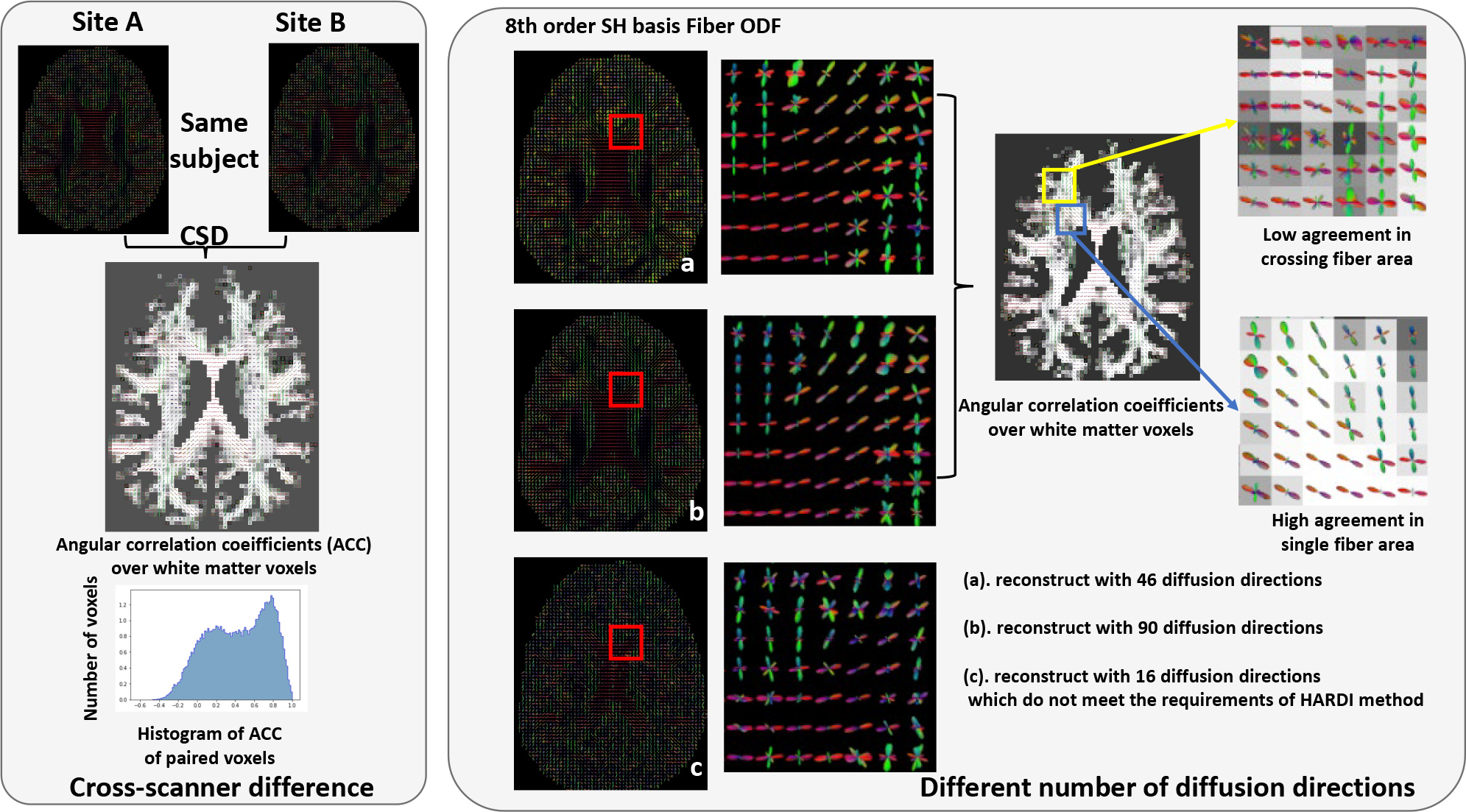
This figure shows that the DW-MRI signals are affected by measurement factors (e.g., hardware, reconstruction algorithms, acquisition parameters). The left panel shows the inter-site variability, even for the data that are collected from the same brain. The right panel shows that the number of diffusion directions impacts the reproducibility of HARDI method (e.g., constrained spherical deconvolution), even in the same acquisition.

Recently, machine learning (ML) and deep learning (DL) techniques have demonstrated their remarkable abilities in neuroimaging.^10,18 Such approaches have been applied to the task of microstructure estimation, aiming to directly learn the mapping between input DWI scans and output fiber tractography while maintaining the necessary characteristics and reproducibility for clinical translation. By not assuming a specific diffusion model, data-driven algorithms can reduce the dependence on data acquisition schemes and additionally require less user intervention. A similar regression approach was presented by Nath et al.,¹⁹ using a multi-layer perceptron (MLP) network for fiber orientation estimation. It presented a deep learning network for estimating discrete fiber orientation distribution functions (FODFs) from voxels of DW-MRI scans.

In this study, we propose a 3D-CNN architecture that utilizes 3 × 3 × 3 cubic patches as the input signals for a single-shell microstructure estimation. The 8^th order spherical harmonics coefficients are used as the voxel-level representation. The scan/rescan data are employed to facilitate our new loss function in reducing the intra-subject variability. Another contribution is that we add intra-subject data augmentation in order to alleviate the impacts of a smaller number of diffusion directions on both reproducibility and the precision of metrics derived from CSD. The method has been trained, validated, and tested on both the HCP young adults (HCP-ya) test-retest group²⁰ and the MASiVar dataset.²¹

2. METHOD

2.1. Data Representation

Spherical Harmonics (SH) are functions defined on the sphere. A collection of SH can be used as a basis function to represent and reconstruct any function on the surface of a unit sphere.²² All diffusion signals are transformed to SH basis signal ODF as a unified input for deep learning models, using 8^th order spherical harmonics with the ‘tournier07’ basis.²³ For the fiber ODF, we processed all the data with single shell single tissue CSD (ssst-CSD) using the DIPY library with its default setting.²² For the spherical harmonics coeifficients $c_k^m$, k is the order, m is the degree. For a given value of k, there are 2m + 1 independent solutions of this form, one for each integer m with −k ≤ m ≤ k. In practice, a maximum order L is used to truncate the SH series. By only taking into account even order SH functions, the above bases can be used to reconstruct symmetric spherical functions, thus, by using order 8^th, we have 45 coefficients for each voxel’s representation.

2.2. Deep Learning Networks

Inspired by Nath et al.,^19,24 we employ a 3D CNN with a residual block and utilize 3×3×3 cubic patches as inputs with the idea that, compared with using signals from single voxel, 3D patches might provide more complete spatial information for deep learning networks(Fig. 2). Briefly, the input size of the network is 3×3×3 in the spatial dimensions by 45 channels, while the outputs are 45 8^th order spherical harmonics coefficients. In this network, three subsequent convolutional layers serve as the critical composition of the CNN with 3D convolution filters. One residual block is included to connect the input and the third convolutional layer. The convolutional filters are then flattened and is connected to two dense layers for predicting FODF at the center voxel locations. All layers are ‘relu’ activated.

Figure 2:

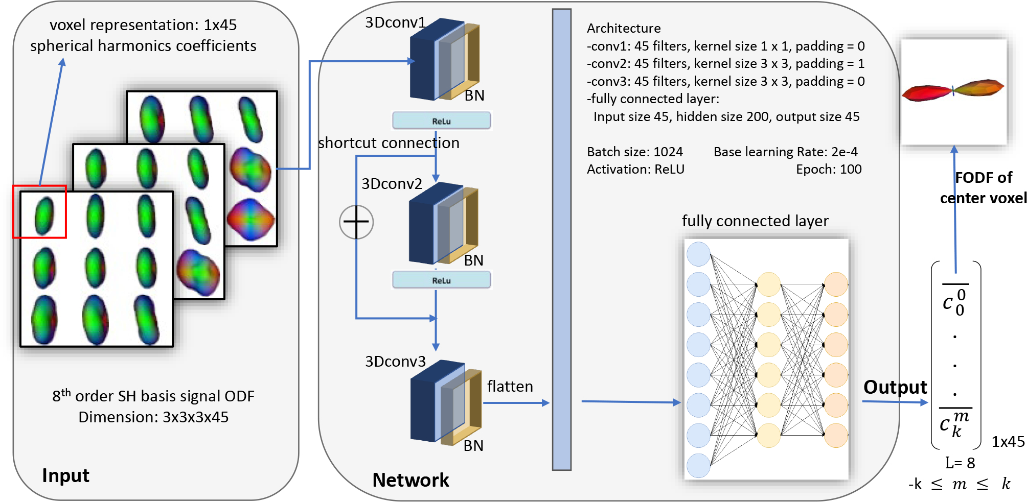
This figure shows the proposed deep learning architecture. We develop a 3D patch-wise convolutional neural network to fit the fiber orientation distribution function (FODF) from the 8^th order spherical harmonics (SH), using 3×3×3 cubic patches.

2.3. Loss Function

We introduce a customized loss function, as shown in Eqs. (1) to (3). The first term is the MSE loss between the network’s FOD prediction and the ground truth with the hyper-parameter ‘α’. N is the number of samples, m is the order of the spherical harmonic (SH) basis and $c_k^m$ is the SH coefficients. The second term is the MSE loss between the paired voxels u, v which is expected to be 0 and the hyper-parameter is ‘β’. To be specific, if no scan/rescan data participate during training, ‘β’ is set to 0.

$$loss1=\frac{1}{N}\sum _{i=1}^N\sum _{k=0}^L\sum _{m=-k}^k{\left({\left(c_k^m\right)}_{true,i}-{\left(c_k^m\right)}_{pred,i}\right)}^2$$ (1)

$$loss2=\frac{1}{N}\sum _{i=1}^N\sum _{k=0}^L\sum _{m=-k}^k{\left({\left(c_k^m\right)}_{u,i}-{\left(c_k^m\right)}_{v,i}\right)}^2$$ (2)

$$Loss=\alpha *loss1+\beta *loss2$$ (3)

2.4. Intra-subject data augmentation

In order to provide a robust microstructure estimation, we introduce intra-subject data augmentation during our network training. In normal acquisition scheme, the b-values of a shell are not all identical, we use tolerance to adjust the accepted interval during shell extraction. Different tolerance of 0, 5, and 20 are applied during single shell extraction to the multi-shell diffusion signal. Thus, we have different numbers of diffusion directions from the same image. The CSD methods are sensitive to the number of diffusion directions. By applying this augmentation, the diffusion ODF generated from fewer diffusion directions (still well distributed on the sphere) is labeled with the CSD results with the full numbers of gradient directions.

2.5. Evaluation metric

To compare the predictions of the proposed deep learning methods we use angular correlation coefficient (ACC, Eq. 4) to evaluate the similarity of the prediction when compared with the ground truth estimate of CSD. ACC is a generalized measure for all fiber population scenarios. It assesses the correlation of all directions over a spherical harmonic expansion. In brief, it provides an estimate of how closely a pair of FODF’s are related on a scale of −1 to 1, where 1 is the best measure. Here ‘u’ and ‘v’ represent sets of SH coefficients.

$$ACC=\frac{{\sum }_{k=1}^L{\sum }_{m=-k}^k\left(u_{km}\right)\left(v_{km}^{*}\right)}{{[{\sum }_{k=1}^L{\sum }_{m=-k}^k{\left|u_{km}\right|}^2]}^{0.5}\cdot {[{\sum }_{k=1}^L{\sum }_{m=-k}^k{\left|v_{km}\right|}^2]}^{0.5}}$$ (4)

3. EXPERIMENTS

The experiments can be summarized as with/without scan/rescan data, and with/without intra-subject augmentation on two deep learning models (voxel-wise MLP presented by Nath et al.¹⁹ and ours in Fig. 2). We assessed the models, as well as benchmarks, using the overall mean ACC on white matter voxels between the prediction and the ground truth. We also conducted an ablation study to examine the robustness of the model when we feed ‘fewer gradient directions’ and compared the results with single shell single tissue CSD (ssst-CSD).

3.1. Data & Data process

For the HCP-ya dataset,²⁰ 45 subjects with the retest acquisition were used (a total of 90 images). The acquisitions at b-value of 2000 s/mm² with 90 gradient directions were extracted for the study. A T1 volume of the same subject was used for WM segmentation using SLANT.²⁵HCP was distortion corrected with topup and eddy.^26,27 Different tolerance of 5, 10 and 20 are applied during single shell extraction as intra-subject augmentation. The mean number of diffusion directions is 90 with a tolerance of 20, 75 with a tolerance of 10 and 60 with tolerance a of 5. 30 subjects are used as training data, while 10 are used for validation and 5 are used for testing.

For the MASiVar dataset,²¹ five subjects were acquired on three different sites referred to as ‘A’, ‘B’ and ‘C’, structural T1 were acquired for all subjects at all sites. All in-vivo acquisitions were pre-processed with the PreQual pipeline²⁸ and then registered pairwise per subject. Two subjects on site ‘A’ and ‘B’ are used as paired training data. One subject is used for validation, while two subjects are used for testing. Acquisitions from site C are used for an ablation study of intra-subject data augmentation which has a mean number of diffusion directions of 72 with a tolerance of 10 and number of 96 with a tolerance of 20. Tolerance of 0 with 16 diffusion directions, as well as a tolerance of 5 with 36 diffusion directions will not be used given that it does not meet the basic requirements for 8^th order CSD reconstruction.

3.2. Voxel-wise experiment

The deep neural network consists of four fully connected layers. The number of neurons per layer is 400, 45,200, and 45. The input is the 1 × 45 vector of the SH basis signal ODF and the output is the 1 × 45 vector of the SH basis Fiber ODF.

The model was trained using the Adam optimizer with a base learning rate of 1e-4. The optimizer learning rate followed (linear scaling²⁹) lr×BatchSize/256. Each experiment was trained for 100 epochs, and the epoch with the lowest loss (equation Eqs. (1) to (3)) over the validation set was used for testing.

3.3. Patch-wise experiment

The architecture in Fig. 2 was used for the patch-wise experiment. The model was then trained using the Adam optimizer with a base learning rate of 2e-4. The optimizer learning rate followed (linear scaling²⁹) lr×BatchSize/256. Each experiment was trained for 100 epochs, and the epoch with the lowest validation loss was used for testing.

4. RESULTS

The results of the FODF estimation are presented in Table. 1. The implementation of the CNN network for 3D-patch inputs has lead to a superior spherical harmonics coefficients estimation by incorporating more information from neighboring voxels. Meanwhile, by introducing the identity loss with scan/rescan data, the performance achieved a higher consistency while maintaining higher angular correlation coefficients with CSD.

Table 1:

Performance of FODF prediction

model & Method	scan/rescan	intra-subject augmentation	mean ACC	inter-scanner consistency
CSD	N/A	N/A	N/A	0.826
			0.942	0.830⋆
voxel-wise	✓		0.938	0.878⋆
	✓	✓	0.939	0.882⋆
			0.949	0.834⋆
patch-wise	✓		0.954	0.886⋆
	✓	✓	0.953	0.891 ⋆

^*Mean ACC are calculated over white matter voxels.

Wilcoxon signed-rank test is applied as statistical assessment (denoted by ⋆). The deep learning performances are statistically significant as compared with baseline–CSD (0.05; p < 0.001).

Ablation study

In the ablation study (Table. 2), we evaluate the intra-subject augmentation by comparing the intra-subject consistency on all white matter voxels with different number of diffusion directions. The deep learning model which has the best performance on the validation set is chosen for comparison. In Fig. 3, the right side shows a qualitative result of the visualization of the estimated SH coefficients and the left side shows the comparison with full-direction CSD. By performing CSD, the test subjects with a mean of 72 diffusion directions can only maintain a mean ACC of 0.848 as compared with their same acquisition with 96 directions. By adding the intra-subject augmentation during the training process, both voxel wise and patch wise models have significant improvement, which shows that deep learning reveals untapped information during the ODF estimation. Fig. 4 shows the result of 1) estimation on a signal with fewer diffusion directions using a patch-wise DL model with scan/rescan data and intra-subject augmentation participated during training and 2) CSD.

Table 2:

Performance in fewer diffusion direction situation

model & method	scan/rescan	intra-subject augmentation	intra-subject consistency
CSD	N/A	N/A	0.848 ± 0.189
			0.838 ± 0.195⋆
voxel-wise	✓		0.849 ± 0.175⋆
	✓	✓	0.879 ± 0.138⋆
			0.842 ± 0.185⋆
Patch-wise	✓		0.856 ± 0.173⋆
	✓	✓	0.902 ± 0.128 ⋆

Wilcoxon signed-rank test is applied as statistical assessment (denoted by ⋆). The deep learning performances are statistically significant as compared with baseline–CSD (0.05; p < 0.001).

Figure 3:

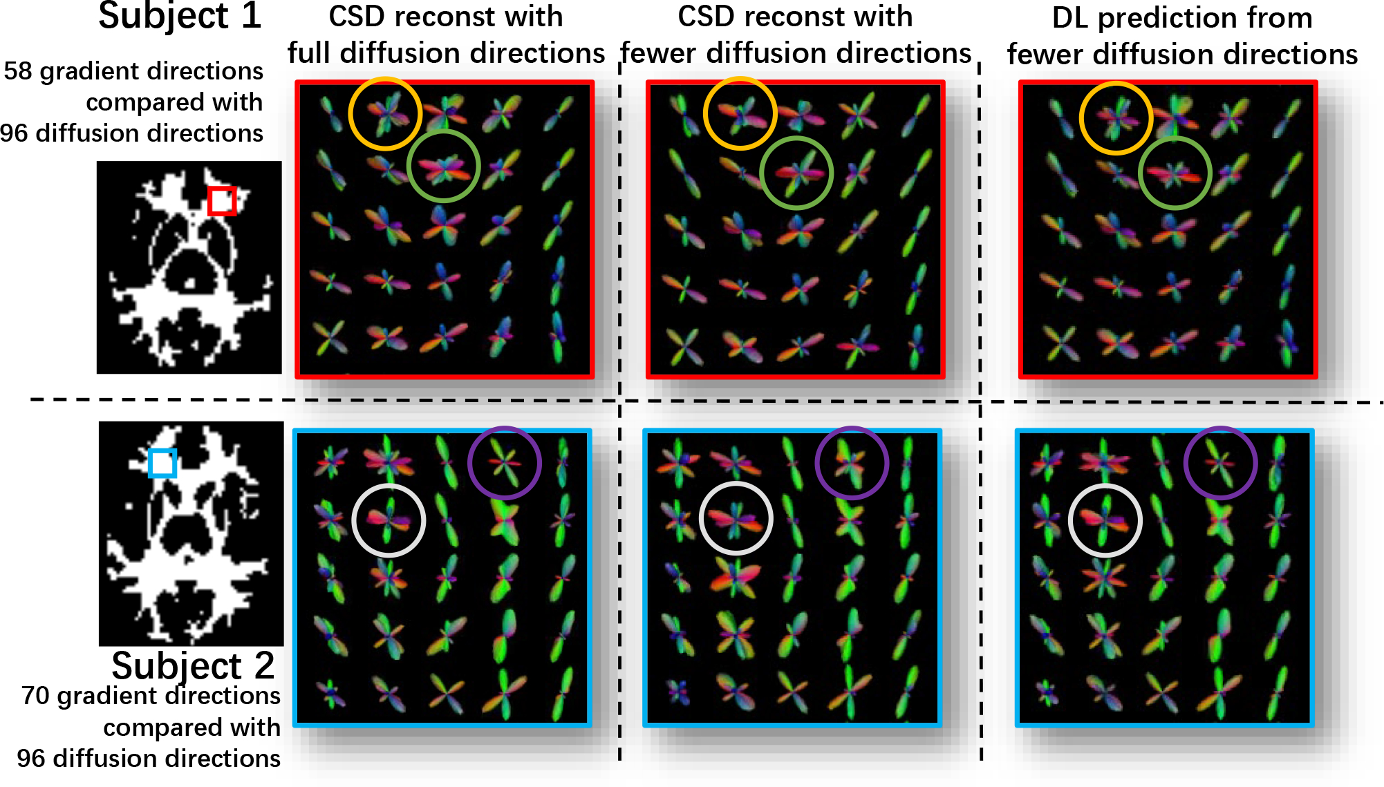
This figure presents the qualitative results of using the proposed deep learning (DL) method, as well as the results from CSD modeling on the 2 testing subjects in MASiVar. Qualitatively, the selected patches show better reconstruction on crossing-fiber areas while the circled spheres indicate better fiber orientation estimation.

Figure 4:

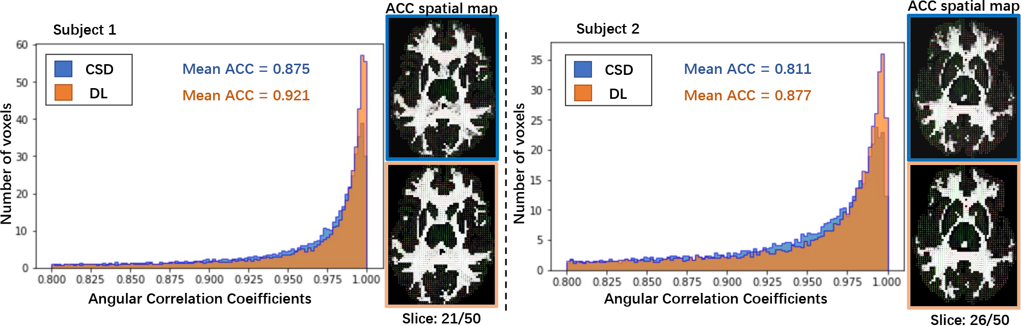
This figure depicts the histogram of ACC between full diffusion directions’ reconstruction and fewer directions’ reconstruction while using the proposed deep learning (DL) method, as well as the results from CSD modeling on the 2 testing subjects in MASiVar. The ACC spatial maps are the comparison between 1) the FODFs of reconstruction from CSD with full diffusion directions and 2) fewer diffusion directions’ CSD and DL estimator on two testing subjects.

5. CONCLUSION

In this paper, we propose a data-driven harmonization algorithms to (1) learn the mapping from SH basis DW-MRI signal to a fiber ODF, (2) improve consistency and alleviate the effects that occur between different scanners, and (3) increase model robustness in the ‘fewer diffusion directions’ scenarios. Our study is a step towards the direct harmonization of the estimated microstructure (FOD) using deep learning and data-driven scheme, when scan-rescan data are available for training. The proposed method is potentially applicable to a wider range of data harmonization problems in neuroimaging.

REFERENCES

- [1].Schaefer PW, Grant PE, and Gonzalez RG, “Diffusion-weighted mr imaging of the brain,” Radiology 217(2), 331–345 (2000). [DOI] [PubMed] [Google Scholar]
- [2].Hagmann P, Thiran J-P, Jonasson L, Vandergheynst P, Clarke S, Maeder P, and Meuli R, “Dti mapping of human brain connectivity: statistical fibre tracking and virtual dissection,” Neuroimage 19(3), 545–554 (2003). [DOI] [PubMed] [Google Scholar]
- [3].Le Bihan D, Mangin J-F, Poupon C, Clark CA, Pappata S, Molko N, and Chabriat H, “Diffusion tensor imaging: concepts and applications,” Journal of Magnetic Resonance Imaging: An Official Journal of the International Society for Magnetic Resonance in Medicine 13(4), 534–546 (2001). [DOI] [PubMed] [Google Scholar]
- [4].Tuch DS, Reese TG, Wiegell MR, Makris N, Belliveau JW, and Wedeen VJ, “High angular resolution diffusion imaging reveals intravoxel white matter fiber heterogeneity,” Magnetic Resonance in Medicine: An Official Journal of the International Society for Magnetic Resonance in Medicine 48(4), 577–582 (2002). [DOI] [PubMed] [Google Scholar]
- [5].Tournier J-D, Yeh C-H, Calamante F, Cho K-H, Connelly A, and Lin C-P, “Resolving crossing fibres using constrained spherical deconvolution: validation using diffusion-weighted imaging phantom data,” Neuroimage 42(2), 617–625 (2008). [DOI] [PubMed] [Google Scholar]
- [6].Jeurissen B, Tournier J-D, Dhollander T, Connelly A, and Sijbers J, “Multi-tissue constrained spherical deconvolution for improved analysis of multi-shell diffusion mri data,” NeuroImage 103, 411–426 (2014). [DOI] [PubMed] [Google Scholar]
- [7].Aganj I, Lenglet C, Sapiro G, Yacoub E, Ugurbil K, and Harel N, “Reconstruction of the orientation distribution function in single-and multiple-shell q-ball imaging within constant solid angle,” Magnetic resonance in medicine 64(2), 554–566 (2010). [DOI] [PMC free article] [PubMed] [Google Scholar]
- [8].Jansons KM and Alexander DC, “Persistent angular structure: new insights from diffusion magnetic resonance imaging data,” Inverse problems 19(5), 1031 (2003). [DOI] [PubMed] [Google Scholar]
- [9].Poulin P, Côté M-A, Houde J-C, Petit L, Neher PF, Maier-Hein KH, Larochelle H, and Descoteaux M, “Learn to track: deep learning for tractography,” in [International Conference on Medical Image Computing and Computer-Assisted Intervention], 540–547, Springer; (2017). [Google Scholar]
- [10].Benou I and Riklin Raviv T, “Deeptract: A probabilistic deep learning framework for white matter fiber tractography,” in [International conference on medical image computing and computer-assisted intervention], 626–635, Springer; (2019). [Google Scholar]
- [11].Essayed WI, Zhang F, Unadkat P, Cosgrove GR, Golby AJ, and O’Donnell LJ, “White matter tractography for neurosurgical planning: A topography-based review of the current state of the art,” NeuroImage: Clinical 15, 659–672 (2017). [DOI] [PMC free article] [PubMed] [Google Scholar]
- [12].Farquharson S, Tournier J-D, Calamante F, Fabinyi G, Schneider-Kolsky M, Jackson GD, and Connelly A, “White matter fiber tractography: why we need to move beyond dti,” Journal of neurosurgery 118(6), 1367–1377 (2013). [DOI] [PubMed] [Google Scholar]
- [13].Jeurissen B, Leemans A, Tournier J-D, Jones DK, and Sijbers J, “Investigating the prevalence of complex fiber configurations in white matter tissue with diffusion magnetic resonance imaging,” Human brain mapping 34(11), 2747–2766 (2013). [DOI] [PMC free article] [PubMed] [Google Scholar]
- [14].Dubey A, Kataria R, and Sinha VD, “Role of diffusion tensor imaging in brain tumor surgery,” Asian journal of neurosurgery 13(2), 302 (2018). [DOI] [PMC free article] [PubMed] [Google Scholar]
- [15].Tournier J-D, Mori S, and Leemans A, “Diffusion tensor imaging and beyond,” Magnetic resonance in medicine 65(6), 1532 (2011). [DOI] [PMC free article] [PubMed] [Google Scholar]
- [16].Tournier J-D, Calamante F, and Connelly A, “Robust determination of the fibre orientation distribution in diffusion mri: non-negativity constrained super-resolved spherical deconvolution,” Neuroimage 35(4), 1459–1472 (2007). [DOI] [PubMed] [Google Scholar]
- [17].Schilling K, Janve V, Gao Y, Stepniewska I, Landman BA, and Anderson AW, “Comparison of 3d orientation distribution functions measured with confocal microscopy and diffusion mri,” Neuroimage 129, 185–197 (2016). [DOI] [PMC free article] [PubMed] [Google Scholar]
- [18].Poulin P, Jörgens D, Jodoin P-M, and Descoteaux M, “Tractography and machine learning: Current state and open challenges,” Magnetic resonance imaging 64, 37–48 (2019). [DOI] [PubMed] [Google Scholar]
- [19].Nath V, Parvathaneni P, Hansen CB, Hainline AE, Bermudez C, Remedios S, Blaber JA, Schilling KG, Lyu I, Janve V, et al. , “Inter-scanner harmonization of high angular resolution dw-mri using null space deep learning,” in [International Conference on Medical Image Computing and Computer-Assisted Intervention], 193–201, Springer; (2019). [PMC free article] [PubMed] [Google Scholar]
- [20].Van Essen DC, Smith SM, Barch DM, Behrens TE, Yacoub E, Ugurbil K, Consortium W-MH, et al. , “The wu-minn human connectome project: an overview,” Neuroimage 80, 62–79 (2013). [DOI] [PMC free article] [PubMed] [Google Scholar]
- [21].Cai LY, Yang Q, Kanakaraj P, Nath V, Newton AT, Edmonson HA, Luci J, Conrad BN, Price GR, Hansen CB, et al. , “Masivar: Multisite, multiscanner, and multisubject acquisitions for studying variability in diffusion weighted mri,” Magnetic resonance in medicine 86(6), 3304–3320 (2021). [DOI] [PMC free article] [PubMed] [Google Scholar]
- [22].Garyfallidis E, Brett M, Amirbekian B, Rokem A, Van Der Walt S, Descoteaux M, Nimmo-Smith I, and Contributors D, “Dipy, a library for the analysis of diffusion mri data,” Frontiers in neuroinformatics 8, 8 (2014). [DOI] [PMC free article] [PubMed] [Google Scholar]
- [23].Tournier J-D, Smith R, Raffelt D, Tabbara R, Dhollander T, Pietsch M, Christiaens D, Jeurissen B, Yeh C-H, and Connelly A, “Mrtrix3: A fast, flexible and open software framework for medical image processing and visualisation,” Neuroimage 202, 116137 (2019). [DOI] [PubMed] [Google Scholar]
- [24].Nath V, Pathak SK, Schilling KG, Schneider W, and Landman BA, “Deep learning estimation of multi-tissue constrained spherical deconvolution with limited single shell dw-mri,” in [Medical Imaging 2020: Image Processing], 11313, 162–171, SPIE (2020). [DOI] [PMC free article] [PubMed] [Google Scholar]
- [25].Huo Y, Xu Z, Xiong Y, Aboud K, Parvathaneni P, Bao S, Bermudez C, Resnick SM, Cutting LE, and Landman BA, “3d whole brain segmentation using spatially localized atlas network tiles,” NeuroImage 194, 105–119 (2019). [DOI] [PMC free article] [PubMed] [Google Scholar]
- [26].Andersson JL, Skare S, and Ashburner J, “How to correct susceptibility distortions in spin-echo echo-planar images: application to diffusion tensor imaging,” Neuroimage 20(2), 870–888 (2003). [DOI] [PubMed] [Google Scholar]
- [27].Andersson JL and Sotiropoulos SN, “An integrated approach to correction for off-resonance effects and subject movement in diffusion mr imaging,” Neuroimage 125, 1063–1078 (2016). [DOI] [PMC free article] [PubMed] [Google Scholar]
- [28].Cai LY, Yang Q, Hansen CB, Nath V, Ramadass K, Johnson GW, Conrad BN, Boyd BD, Begnoche JP, Beason-Held LL, et al. , “Prequal: An automated pipeline for integrated preprocessing and quality assurance of diffusion weighted mri images,” Magnetic resonance in medicine 86(1), 456–470 (2021). [DOI] [PMC free article] [PubMed] [Google Scholar]
- [29].Goyal P, Dollár P, Girshick R, Noordhuis P, Wesolowski L, Kyrola A, Tulloch A, Jia Y, and He K, “Accurate, large minibatch sgd: Training imagenet in 1 hour,” arXiv preprint arXiv:1706.02677 (2017). [Google Scholar]