Abstract
Background and Objective
Respiratory diseases caused by viruses are a major human health problem. To better control the infection and understand the pathogenesis of these diseases, this paper studied SARS-CoV-2, a novel coronavirus outbreak, as an example.
Methods
Based on coupled computational fluid and particle dynamics (CFPD) and host-cell dynamics (HCD) analyses, we studied the viral dynamics in the mucus layer of the human nasal cavity-nasopharynx. To reproduce the effect of mucociliary movement on the diffusive and convective transport of viruses in the mucus layer, a 3D-shell model was constructed using CT data of the upper respiratory tract (URT) of volunteers. Considering the mucus environment, the HCD model was established by coupling the target cell-limited model with the convection-diffusion term. Parameter optimization of the HCD model is the key problem in the simulation. Therefore, this study focused on the parameter optimization of the viral dynamics model, divided the geometric model into multiple compartments, and used Monolix to perform the nonlinear mixed effects (NLME) of pharmacometrics to discuss the influence of factors such as the number of mucus layers, number of compartments, diffusion rate, and mucus flow velocity on the prediction results.
Results
The findings showed that sufficient experimental data can be used to estimate the corresponding parameters of the HCD model. The optimized convection-diffusion case with a two-layer multi-compartment low-velocity model could accurately predict the viral dynamics.
Conclusions
Its visualization process could explain the symptoms of the disease in the nose and contribute to the prevention and targeted treatment of respiratory diseases.
Keywords: Viral dynamics, SARS-CoV-2, Parameter optimization, Mucus layer, Computational fluid-particle dynamics, Host-cell dynamics
1. Introduction
Due to the outbreak of the novel coronavirus disease (COVID-19) and relevant popular science, respiratory diseases are no longer an unfamiliar topic. Other diseases caused by respiratory viruses, such as Influenza-A, MERS-CoV, and Ebola are also well-known threats to human health. To understand the infection dynamics and pathogenesis of these viruses, we used the severe acute respiratory syndrome coronavirus 2 (SARS-CoV-2), which causes COVID-19, as an example to perform research because of the most recent global pandemic [1].
Clinical data are indispensable for studying the nature and infection mechanisms of SARS-CoV-2. Modern viral dynamics modeling and its success in human immunodeficiency virus (HIV) research have allowed viral dynamics modeling to be extended to study a large number of other viral infections. Therefore, researchers use the host-cell dynamics (HCD) approach, based on clinical data, to predict viral loads and better understand viral replication and the host immune response during infection. HCD refers to the complex interplay between a virus and the cells it infects [2]. When a virus enters a host cell, it hijacks the cellular machinery to replicate itself, which can lead to damage to the host cell and potentially cause disease [3]. The host cell, in turn, mounts a response to the virus, which can involve various immune cells and signaling pathways [4]. The dynamics of this relationship between virus and host cell can be influenced by a variety of factors, including the characteristics of the virus (such as its structure and replication cycle), the properties of the host cell (such as its receptors and immune response), and environmental factors (such as temperature and pH) [5]. Understanding host cell dynamics is important for developing treatments and vaccines for viral diseases. By studying the mechanisms of viral infection and the host response, researchers can identify potential targets for therapies and gain insights into how the immune system can be harnessed to combat viral infections [6]. Previously, Wang et al. [7] conducted a cohort trial with 23 patients of varying ages to investigate viral loads using reverse transcriptase quantitative PCR (RT-qPCR) when the exact mechanism was unknown. They discovered that the highest viral load in saliva occurred during the first week after symptom onset, and then declined. Additionally, they observed that older patients had higher viral loads. This was different, however than the findings of a study by Wölfel et al. [8], who found that the peak viral load, measured by throat swabs, was four days after symptom onset in nine cases, indicating that viral load is variable and dependent on the individual. They also found that SARS-CoV-2 was not only detectable in the lower respiratory tract (LRT), but also actively replicated in the upper respiratory tract (URT). Considering the different times of infection onset, Hernandez-Vargas et al. [9] proposed a dynamic mathematical model including immune cell responses that best represented the fitting data of SARS-CoV-2 in infected patients based on the target-cell limited (TCL) model, and the data of Wölfel et al. [8], which predicted that the replication of SARS-CoV-2 was likely to be slow at the beginning of infection. Gastine et al. [10] established a viral dynamic dataset based on patient-level data on viral load from 645 patients aged 1 month to 100 years and used a multivariate Cox proportional hazard (Cox-pH) regression model and a simplified four-parameter nonlinear mixed effects (NLME) model to estimate viral clear time and fit viral load tracks to the sampling sites, respectively. They indicated that virus clearance took longer in older patients, men, and patients with more severe diseases, and that related drugs were associated with rapid clearance of the virus. Similar conclusions were reached in a study by Neant et al. [11], in which the mortality and virological information from 655 hospitalized patients were analyzed. The TCL model with an eclipse phase, immune responses, and empirical Bayesian estimation (EBE) of individual parameters using non-parametric tests were used to estimate relevant parameters and assess risk factors. The model predicted median viral load peaks coinciding with symptom onset and simulated the effects of effective drug interventions on viral clearance time and mortality. The results showed that viral dynamics correlated with mortality in hospitalized patients. Because the SARS-CoV-2 viral load changes rapidly, Agyeman et al. [12] used five different modeling methods to fit the two datasets [10,11] starting within 7 days of symptom onset and evaluated their performance. They suggested that simple models should be considered for the development of the pharmacodynamic model. However, the development of a suitable pharmacodynamic model for SARS-CoV-2 needs to be explored. Perelson et al. [13] reviewed the historical development of mathematical models and highlighted recent contributions to the application of these models to understand SARS-CoV-2 infection, emphasizing the power of the simple TCL model and its evolution into more complex models capable of capturing greater detail. Robinot et al. [14] investigated the functional and structural consequences of SARS-CoV-2 infection in a reconstructed model of the human bronchial epithelium. SARS-CoV-2 replication causes a temporary decline in epithelial barrier function, and epithelial antiviral defense mechanisms (including basal cell mobilization and interferon induction) are overwhelmed and disrupted by active viral replication. Therefore, based on the TCL model, the immune response phase seems to be less important for predicting virus dynamics.
Although a single mathematical model based on empirical parameters can roughly describe the trend of the viral load, it is still insufficient to describe the specific dynamics and hotspots of SARS-CoV-2 in the respiratory tract. To further delineate and visualize virus dynamics, computational fluid-particle dynamics (CFPD) can be considered as a promising approach coupled with the HCD model. As mentioned previously, the ability of SARS-CoV-2 to actively replicate in the URT has attracted widespread attention. Hofer et al. [15] suggested that COVID-19 begins when people inhale respiratory aerosols that contain virions. Therefore, the distribution of inhaled virus-laden particles is an influential initial condition for predicting viral dynamics in the respiratory tract. Guo et al. [16] simulated the transportation and deposition of droplets of 1–50 μm in diameter released from the trachea or bronchus during exhalation using a real reconstruction model of the human respiratory tract. They showed that droplet deposition was mainly affected by the droplet diameter and exhaled flow rate, and the larger the flow rate, the fewer the droplets released into the environment. For inhalation, based on CFD and fluid-solid interaction (FSI), Mortazavi et al. [17] studied the airflow field during human URT SARS-CoV-2 microdroplet injection in a well-validated real anatomical model from Computer Tomography (CT) data and used a discrete phase model (DPM) to solve the field. An accurate assessment of the temporal and spatial motion of the deposits in virus-impregnated droplets was obtained by means of in vitro DPM in the upper respiratory system with oral inhalation, which showed that the amount of microdroplet deposition in the nasal cavity was less when only inhaled through the mouth, but the stay time was long. However, nasal breathing physiologically dominates in daily life; therefore, they conducted another study [18], in which they used the physical properties of SARS-CoV-2 to study droplet behavior and deposition patterns during nasal inhalation. They attempted to simulate the process by which viral droplets of 1–10 μm inhaled through the nose were deposited in the URT. The model suggested that viral droplets accumulate in the nasal cavity and remain in the upper turbinate for a long time, interfering with the subjects' olfaction. With an increase in the flow rate and droplet diameter, the URT contamination process increased. Similarly, by establishing and studying two airway models created using CT data, Phuong et al. [19] predicted the total deposition and regional deposition of particles with 1–10 μm aerodynamic diameters in an actual human URT under nasal inhalation and demonstrated the influence of the interdisciplinary variation of deposition fractions. Further, considering the practical application of respiratory model for inhalation exposure risk assessment, Yoo et al. [20] used the experimental results of PIV on the replica URT model to verify the prediction accuracy of particle transport and deposition analysis.
The study of virus dynamics should not stop with the deposition of virion-carrying particles in the respiratory tract using CFPD. It is possible to carry out a series of activities, such as convection, diffusion, infection of target cells, replication, and removal, along with the mucus flow of the mucus layer after the virus is deposited in the URT mucosa [21]. With the progress of related research, host cells with angiotensin-converting enzyme 2 (ACE2) and transmembrane protease serine 2 (TMPRSS2) as the receptor and coreceptor, respectively, are considered to be a breakthrough in SARS-CoV-2 invasion [22], [23], [24], which is of guiding significance for the selection of target cells in its dynamic prediction. Therefore, the mucus layer acts as the first line of defense against inhaled unwanted particles [25] and the function of mucociliary movement should not be underestimated. Because the diameter of drug particles is similar to that of SARS-CoV-2 and other coronaviruses (approximately 100 nm) [26], CFD methods considering the mucus layer used in intranasal drug delivery can be used as a reference in viral dynamics research. There are two common models: one is the method used by Rygg et al. [22] to convert three-dimensional (3D) nasal geometry into a surface-based two-dimensional (2D) model, calculate its mucus velocity field, and verify it with the in vivo nasal clearance rate. This study established a complete CFD model of nasal aerosol delivery, from the point of spray formation to the respiratory epithelial surface for absorption. Second, Shang et al. [27] built a 3D-shell model based on the actual geometric shape of the nasal cavity. Shang also conducted a comparative study [28] on the two methods and found that the results of the 3D-shell model were in better agreement with the experimental data. Hence, in our previous study [29], a 3D-shell CFPD-HCD model coupled with the convection-diffusion term was used to understand the viral infection dynamics in the mucus layer. However, the parameters used in that study from clinical data fitting did not apply to the developed model because the predicted trends were slightly different from the clinical data values, which means that this model is highly sensitive to the initial conditions and parameters. Therefore, parameter optimization and dataset selection are worth exploring.
In this study, the existing model [29] was further improved based on the properties of the respiratory mucus layer. Here, the SARS-CoV-2 human challenge dataset [30] without drug treatment with a clear date of virus inoculation was selected for parameter fitting optimization by Monolix [31,32]. The viral dynamics over time in the nasal cavity-nasopharynx were visualized in the 3D-shell model by the CFPD method, which will contribute to the prevention and region-specific treatment of COVID-19.
2. Methods
Here, we describe in detail the improved HCD model, the initial condition settings, and the optimization of related parameters and influencing factors. The establishment of the 3D-shell model used for CFPD simulation has been detailed in previous studies [29].
2.1. Model review and initial conditions settings
The HCD model developed in this study is a simple target-cell-limited model combined with a convection-diffusion term. Fig. 1 shows a series of processes that occur after the deposition of virus-laden particles into the mucus layer. The mucus layer can be divided into two layers [33,34] with an upper high-viscosity gel layer and a lower low-viscosity sol layer. When viruses are released into the mucus, they carry out convection and diffusion, along with mucus flow. Additionally, when they bind to the receptors on the target cell surface, they commence infection, replication, re-release, clearance, and apoptosis.
Fig. 1.
Combination of the HCD model and the convection-diffusion term in the mucus layer.
The formula corresponding to the above figure [29] is as follows:
| (1) |
| (2) |
| (3) |
where T, I, and VL are the number of target cells, number of infected cells, and viral load, respectively. As for the parameters involved in the equations, it is assumed that SARS-CoV-2 infects susceptible target cells at β (copy /mL/ day) rate. Infected cells are cleared at δ (day−1) rate due to cytopathic viral effects and immune responses. Meanwhile, c (day−1) and p' (copy/day/cell) represent the rate at which the virus is cleared and the rate at which the infected cell produces and releases the virus, respectively. Vm (mL) represents the mucus volume obtained by multiplying the surface area and thickness of the mucus. In addition, (m/s) is the average flow velocity of mucus in the nasal cavity-nasopharynx. The nasopharyngeal outlet velocity of the model was set to 0.000167 m/s (10 mm/min), which is normal to the boundary within the range (8–10 mm/min) of mucus flow at the posterior of the nasal cavity as Shang et al. mentioned [28]. Dv (m2/s) is the diffusion coefficient of SARS-CoV-2 into the mucus layer. Assuming that the temperature T in the airway is constant at 310 K, and the viscosity of water μ 0 at this temperature is 0.00071 Pa·s, then Dv can be estimated as follows:
| (4) |
| (5) |
where D0 (m2/s) is the diffusion coefficient of SARS-CoV-2 in water estimated by the Stokes-Einstein equation, and rv, rf, and rg represent the effective radius of SARS-CoV-2 (5 × 10⁻⁸ m), the radius of mucin fibers in mucus (3.5 × 10⁻⁹ m), and effective reticular fiber spacing of the mucin network (5 × 10⁻⁸ m), respectively. kB represents the Boltzmann constant (1.380649 × 10⁻²³ J/K). Furthermore, the density ρ of 1000 kg/m3 and viscosity μ of 12 Pa·s were set to describe the mucus properties, and the source term Sm was coupled into the continuity equation for the mucus domain [27]:
| (6) |
Previous studies have proven that the HCD model is sensitive to initial conditions and parameter settings. With a deep understanding of the SARS-CoV-2 infection mechanism, it is estimated that approximately 20% of respiratory epithelial cells express ACE2 receptors and TMPRSS2 coreceptors [35]. These cells may become susceptible to SARS-CoV-2 infection. The number of epithelial cells in the airway was calculated based on the surface area of the airway and the surface area of each epithelial cell, which was assumed to be 4 × 10–11 m2/cell [36]. The initial number of target cells, T(0), was estimated based on this information. The initial number of infected cells I(0) was assumed to be 0.
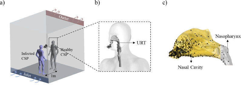
The initial VL(0) was estimated based on the distribution of droplets deposited in the nasal cavity-nasopharynx (evaporation or condensation were not considered here), and the initial viral load value was calculated based on the amount of virus carried by droplets of different sizes. For the deposition of droplets, we referred to our previous studies [37,38] and briefly introduced the simulation method here, we used the droplet deposition results as one of the initial conditions in this study. As shown in Fig. 2 a, we assumed that two computer-simulated persons (CSPs) stand face-to-face in a 3 × 3 × 3 m3 displacement-ventilated space. Considering the worst-case scenario, we assumed that an infected patient (purple CSP near the air inlet) coughs once, and a healthy susceptible person (gray CSP opposite the infected person near the air outlet) is simultaneously taking a 4 s cycle of nasal breathing, where they were 1 m apart without wearing masks. To obtain the distribution of virus-laden droplets in the URT of susceptible individuals, a 3D-URT model based on CT data was combined with the healthy CSP, which was depicted in Fig. 2b. Based on the total number of droplets produced in a cough and the distribution of droplet sizes, it was estimated that 45,000 particles with a size range of 1–10 μm, accounting for approximately 70% of the droplets produced in a cough [29,39,40], were generated from the mouth of the infected CSP. Lagrangian tracking analysis of the particles was then performed using the transient simulation of CFPD. The results showed that more than 90% of the inhaled droplets were deposited in the nasal cavity-nasopharynx, as shown in Fig. 2c, which also proved that it was reasonable and necessary to study this part of the URT.
Fig. 2.
Initial viral load VL(0) acquisition process. a) Infection scenario hypothesis, b) Healthy CSP with a 3D-URT, c) Droplets deposition.
2.2. Parameter optimization
Optimizing the parameters such as β, δ, c and p’ in the model is crucial for accurately representing the biological system, calibrating the model to experimental data, performing sensitivity analyses, comparing different models, and guiding the development of new treatments. By optimizing these parameters, the model can more accurately represent the dynamics of the host-pathogen interaction. This can lead to better understanding of the underlying biological processes and help guide future research or treatments. Therefore, based on non-linear mixed effects modeling (NLME) for pharmacometrics, Monolix software was used to fit the SARS-CoV-2 human challenge dataset to optimize the parameters in the HCD model, and then the optimized parameters were introduced into ANSYS/Fluent (ANSYS Inc.) [41] for visual simulation. Experimental data were also used to validate the accuracy of the simulation results.
First, the geometric model of the nasal cavity-nasopharynx was preliminarily divided into k compartments with equal surface areas. Three cases of k = 1, 10, and 20 were considered, as shown in Fig. 3 .
Fig. 3.
Model partitioning modes. a) 1 compartment, b) 10 compartments, c) 20 compartments.
Second, for the models with different partitioning modes, the initial conditions were determined according to T(0), I(0), VL(0), and k. Because the compartments had the same surface area, the initial number of target cells in each compartment was assumed to be equal to Tk(0), that is, the quotient of T(0) and k. The initial number of infected cells Ik(0) was also 0, whereas the initial viral load VLk(0) was obtained according to the deposition location of the droplets and the amount of virus contained in the droplets. In addition, the effect of the number of layers on the fitting results was considered according to the properties of the mucus layers, as detailed below.
2.2.1. One-layer multi-compartment model
First, the mucus layer was simplified into one layer and its rationality was verified [28]. Here, 15 μm, within a reasonable range, was selected as the thickness of the mucus layer. Since the mucus in the URT flows to the pharynx [25], it was assumed that the mucus flows from the vestibule to the nasopharynx, with the nasopharynx as the exhaust outlet.
As shown in Fig. 4 , SARS-CoV-2 replicated in the infected cells and was released into the mucus layer, which diffused and convected the mucus flow. Hence, the original model was updated using the following calculation process:
| (7) |
| (8) |
| (9) |
where Tk, Ik, and VL,k represent the number of target cells, number of infected cells, and viral load dynamically changing over time in each compartment, respectively. Vm ,k, and Q express the mucus volume in each compartment and the flow velocity of mucus between adjacent compartments, and the latter is estimated by the product of the outlet area and velocity.
Fig. 4.
Schematic diagram of the viral dynamics with the one-layer multi-compartment model.
2.2.2. Two-layer multi-compartment model
A two-layer model of the mucus layer, close to the realistic physiological structure, was also considered, namely, a gel layer of 5 μm and a sol layer of 10 μm.
As shown in Fig. 5 , the mucus in the sol layer is relatively stationary owing to the existence and rhythmic oscillations of the cilia. On the other hand, the mucus in the gel layer flows because the kinetic energy of cilia movement is transferred to the gel layer. Based on this, it was assumed that only diffusion motion occurred after the infected cells released the virus into the sol layer, and convection occurred with the mucus flow after diffusion into the gel layer. Therefore, the original model was further refined and improved using the following equations:
| (10) |
| (11) |
| (12) |
| (13) |
Fig. 5.
Schematic diagram of the viral dynamics with the two-layer multi-compartment model.
Similarly, VL,sol,k, VL,gel,k, Vsol,k, and Vgel,k represent the viral load and mucus volume of the sol and gel layers in each compartment, respectively. Then, Δx and Ak express the distance between the center of the sol and gel layers and the interface area between the sol and gel layers in each compartment, respectively.
2.2.3. Considerations for other factors
In the case of a 20-compartment geometric model, the influence of the selection of virus diffusivity in mucus and mucus velocity on the predicted results of the viral load simulation was further discussed.
In the diffusion cases, three different diffusion coefficients (Dv1, Dv2, and Dv3) were considered, based on the estimation methods proposed by various researchers. Dv1 (2.91 × 10⁻¹² m2/s) is the diffusion coefficient of the virus in the mucus layer calculated by Eqs. (4) and (5) [27,29,42]. Dv2 (6.40 × 10⁻¹² m2/s) is assumed to be the diffusion coefficient of the virus in water calculated by Eq. (5), similar to that in mucus [43]. Finally, Dv3 (5.33 × 10⁻¹⁶ m2/s) is the diffusion coefficient in the mucus layer directly calculated using Eq. (5), but replacing μ 0 with μ [21] , respectively.
In the convection-diffusion cases, the simulated prediction of viral load may be sensitive to the flow velocity of the mucus. Accordingly, three different mucus flow velocities were selected, U1, U2, and U3 with values of 10, 5, and 1 mm/min, respectively. The reason for this choice was that the mucus layer of patients would thicken to varying degrees after being infected with COVID-19. With the thickening of the mucus layer, it would be increasingly difficult for the mucociliary movement to drive the gel layer to flow [44]. Therefore, lower-than-normal mucus flow velocities were carefully selected for comparative analysis.
3. Results
3.1. Effects of the number of layers and compartments
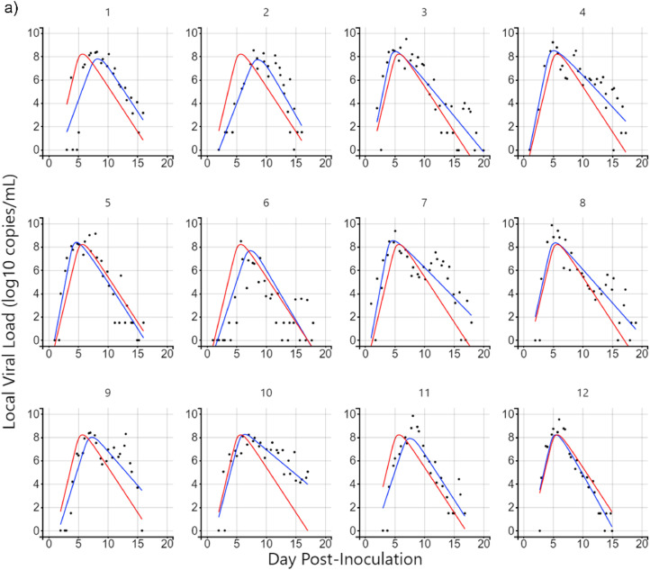
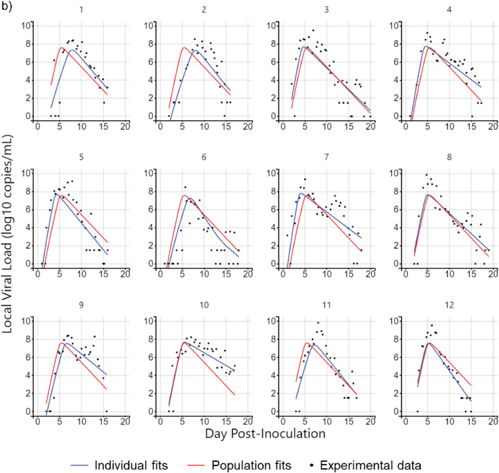
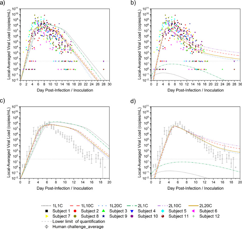
Twelve cases were considered according to the model with different numbers of layers and compartments, convection, and diffusion. Monolix was used to parameterize 20-day viral load data from the nasopharyngeal swabs of 12 untreated subjects in a previous study [30]. The diffusion case with one-layer 20-compartment (1L20C) in Fig. 6 a and the convection-diffusion case with two-layer 20-compartment (2L20C) in Fig. 6b are exemplified.
Fig. 6.
Illustration of parameter fitting by Monolix. a) Diffusion case-1L20C, b) Convection-diffusion case-2L20C.
The red curve represents the population fits of the 12 subjects using different combinations of parameters in different cases, whereas the blue curve represents individual fitting, and each person has their parameter values, the distribution of which is shown in Fig. 7 .
Fig. 7.
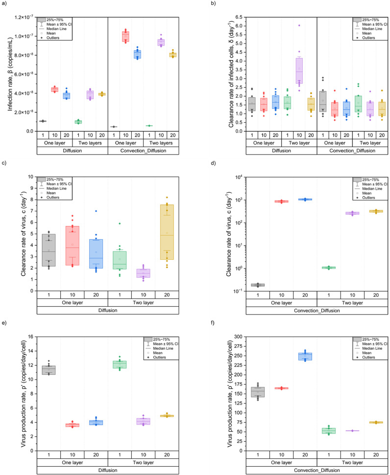
Parameter distribution in all cases with individual fits.
According to the analysis, the infection rate, β, in the convection-diffusion cases was slightly higher than that in the diffusion cases but was concentrated in the ∼ × 10−8 order of magnitude, whereas the values were lower in the 1C cases. Moreover, the clearance rate of infected cells, δ, was mostly in the range of 1–2 day−1 except in a few cases. However, the distribution of the values of virus clearance, c, and virus production of infected cells, p', which differed greatly in the diffusion and convection-diffusion cases, need to be learned separately at this time. In the diffusion cases, the average value of c was less than 5 day−1, and the overall distribution ranged from 0 to 10 day−1, with slightly large individual differences. Nevertheless, the values of p' were concentrated around 4 copies/day/cell, except in the 1C cases with higher values, which were distributed in 10–14 copies/day/cell. In the convection-diffusion cases, the distribution of c values spanned four orders of magnitude. In the 1C cases, the value was a single digit, whereas in other cases, the values of c could reach more than ∼103 day−1. The p' values were also high, the results were relatively stable in the 2 L cases, and the distribution was within 100 copies/day/cell. This finding might be related to the phenomenon of convection caused by mucus flow, which merits further investigation.
Because the individual fitting was dependent on the physical conditions of different subjects, this study incorporated the parameter values derived from the population fitting into the models to obtain more universal predictions, which were the local viral load in the nasopharynx depicted in Fig. 8 .
Fig. 8.
Comparison of the effects of the number of layers and compartments on parameter fitting. a) Diffusion cases with individual data, b) Convection-diffusion cases with individual data, c) Diffusion cases with average data, d) Convection-diffusion cases with average data.
As can be seen from Figs. 8a and b, except for 1C cases, prediction curves fell within the scatter range of the experimental data, which reflected that the 1C models were not reliable and ignored details of mucus flow. Therefore, 1C models could be removed from the following studies and not taken into consideration. Owing to the scattered data points, it was difficult to judge whether the prediction was good or not. Therefore, the average value of the human challenge experiment data was selected in Fig. 8c and d for a clearer comparison.
Further analysis showed that the predictions of these cases were consistent with the experimental data in the slope of the viral load increase stage, the peak time (4–6 days after infection), and the order of magnitude of the peak value (∼ × 108 copies/mL). The values of the 2 L cases were slightly higher than those of the 1 L cases. Among them, diffusion case-1L20C and convection-diffusion case-2L20C performed better; that is, they were closer to the experimental data. However, at the peak and decline of viral load, the diffusion cases began to behave differently from the convection-diffusion cases. For the diffusion cases, the viral load continued to decline for approximately one week after it reached the peak, which gradually deviated from the experimental data, although the slope of the decline was close to that of the experimental data. Nevertheless, the best case was still 1L20C. For the convection-diffusion cases, the predicted values were in good agreement with the experimental data in the initial stage of viral load decline, but the slope gradually changed gently before dropping below the detection limit, which might be associated with mucus consistently maintaining a high velocity. Among them, the 20C cases showed the best performance. In summary, among the cases in this section, 1L20C and 2L20C were well fitted to the diffusion and convection-diffusion cases, respectively, as shown in Fig. 9 . The parameter values obtained by population fitting in the corresponding models are summarized in Table 1 .
Fig. 9.
Visualization of the viral dynamic in the well-fitted cases.
Table 1.
Population fitting of parameters corresponding to well-fitting cases.
| Well-fitting cases | β (copies/mL/day) | δ (day−1) | c (day−1) | p' (copies/day/cell) |
|---|---|---|---|---|
| Diffusion Case-1L20C | 3.81 × 10⁻⁸ | 1.78 | 2.76 | 4.05 |
| Convection-Diffusion Case-2L20C | 8.10 × 10⁻⁸ | 1.22 | 314.00 | 74.50 |
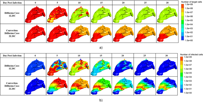
As shown in Fig. 9, when only diffusion was considered, the hot spots where virus-laden droplets deposited and released the virus were taken as the center for diffusion. In the early stage, the viruses concentrated in the vestibule gradually spread to the whole nasal cavity and nasopharynx, in addition to a small residue in the superior nasal concha (ethmoid) [45] in the late stage. However, when convection and diffusion were considered simultaneously, the viruses spread along with mucus flow and gradually flowed to the nasopharynx. In the later stage, the viruses mainly remained around the nasal concha in the central nasal passage, which might be because the complex structure of the nasal bone led to slow flow velocity in the middle part, resulting in the accumulation of the viral load.
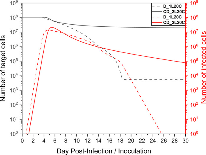
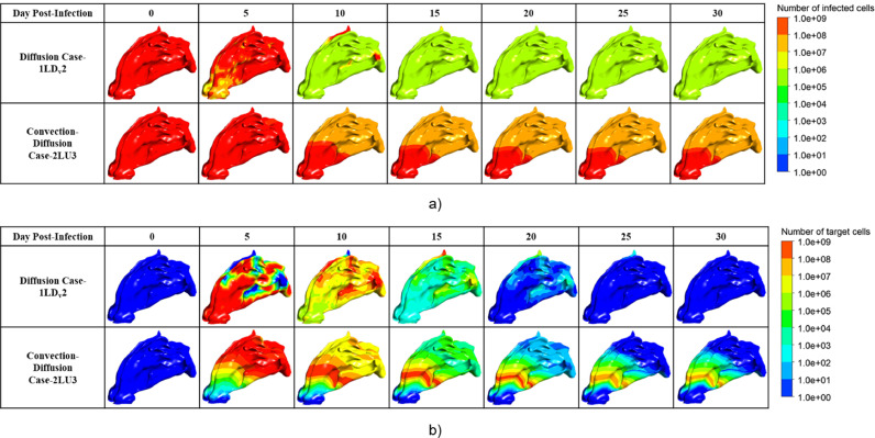
By further analyzing the time series of the number of healthy target cells and infected cells in Fig. 10 , it was found that when only diffusion existed, the infected cells were cleared within a month, whereas the convection-diffusion case did not have a large number of infected cells cleared within a month, as shown in Fig. 11 a. After the peak viral load, the number of infected cells decreased; however, the slope was small. Notably, as shown in Fig. 11b, there was still a high number of infected cells in the front of the nasal cavity, and the virus continuously released by these cells might still have a high risk of infecting the target cells, which would explain why the virus remained near this site.
Fig. 10.
Time series of distribution of a number of target/infected cells in the well-fitted cases.
Fig. 11.
Visualization of the distribution of the number of a) target cells and b) infected cells in the well-fitted cases.
Moreover, the model fitting parameter values of the two cases in Table 1, β and δ, were in line with expectations. However, for c and p', the convection-diffusion case-2L20C was relatively large and was closely related to the mucus flow velocity. Since the viral load was quickly cleared with mucus flow, to better fit the experimental data, the production rate would increase, as did the rate of virus clearance.
According to these results, it was found that the convection-diffusion models were relatively sensitive to the mucus velocity, which was then analyzed and discussed. Thought was also given to the question of whether the models of diffusion cases were dependent on the diffusive rate.
3.2. Effects of diffusive transport and mucociliary clearance
Following the methods mentioned in Section 2.2.3, the influences of the diffusive rate and mucus flow velocity on the model prediction of diffusion cases and convection-diffusion cases are discussed.
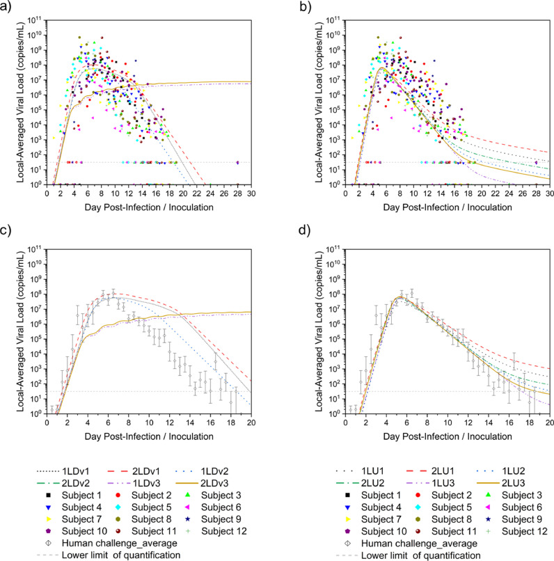
The estimation of the diffusion coefficient of the virus in mucus has a significant influence on the simulation results of diffusion cases. As shown in Fig. 12 a, the smaller the diffusion coefficient, the slower the virus would spread outward from the hot spots, so it took longer to reach the peak, and longer peak periods lead to long-term attenuation, which was particularly obvious when the diffusion rate was Dv3. Fig. 12c more clearly shows the fit between the attenuation process of each case and the experimental data, which indicates that diffusion case-1LDv2 was superior.
Fig. 12.
Comparison of the effects of the diffusive rate and velocity on parameter fitting. a) Diffusion cases with individual data, b) convection-diffusion cases with individual data, c) diffusion cases with average data, and d) convection-diffusion cases with average data.
Likewise, mucus flow velocity also had a certain degree of influence on the predicted viral dynamic results of convection-diffusion cases. As shown in Fig. 12b, the velocity values had an insignificant effect on the predicted results before the viral load peaked; however, a specific difference in the decline period began to appear. Fig. 12d shows that the lower the mucus flow velocity, the closer the decline slope of the viral load was to the slope of the diffusion condition; that is, the higher the degree of fit with the experimental data. This was related to the aforementioned thickening of the mucus layer of the patient's airway, leading to the gradual failure of the movement of mucus cilia. The final movement of the viruses in the mucus layer may be mainly diffusion. Fig. 13 provides a detailed comparison of the flow velocity distribution in the entire nasal cavity-nasopharynx model under different outlet flow velocities. Although the results of the convection-diffusion case-1LU3 were closer to the experimental value in the later stage, they lagged behind 2LU3 when the viral load rose to the peak stage, which was highly valued in the early clinical stage.
Fig. 13.
Mucus flow field of convection-diffusion cases with outlet velocity in a) 10 mm/min, b) 5 mm/min, and c) 1 mm/min.
In all cases, the viral load prediction results were slightly higher in the two-layer model, possibly because it described the nature of the real mucus layer and the mechanism by which the virus moved within it in more detail. According to the above results, the viral load changes in the two cases with better performance within one month are reproduced in Fig. 14 . The corresponding parameters of population fitting are summarized in Table 2 .
Fig. 14.
Visualization of the viral dynamic in the better-fitted cases.
Table 2.
Population fitting of parameters corresponding to better-fitting cases.
| Better-fitting cases | β (copies/mL/day) | δ (day−1) | c (day−1) | p' (copies/day/cell) |
|---|---|---|---|---|
| Diffusion Case-1LDv2 | 4.70 × 10⁻⁸ | 1.53 | 3.62 | 3.44 |
| Convection-Diffusion Case-2LU3 | 4.00 × 10⁻⁸ | 1.38 | 41.73 | 21.37 |
The viral dynamic images in Fig. 14 are similar to those shown in Fig. 9. For diffusion case-1LDv2, the higher diffusive rate accelerates the process of the virus spreading through the nasal cavity and nasopharynx and its clearance. The convection-diffusion case-2LU3 reduced the proportion of convection so that the viruses did not flow away with the mucus quickly, highlighting the effect of diffusion. In addition, because of the slow flow of mucus in the central nasal passage, as shown in Fig. 13c, the viruses might be more likely to remain there, which could also contribute to nasal congestion or olfactory dysfunction, since the olfactory nerve is located nearby [46]. Therefore, it would be better to suggest that detection may occur at other sites within the nasal cavity because current analyte detection using swabs is generally performed from the pharynx or nasopharynx.
Similarly to Fig. 10, when only diffusion existed, the infected cells were cleared within a month, and the increase in the diffusion coefficient shortened the time for the infected cells to be cleared, as shown in Fig. 15 . For the convection-diffusion case with the optimal fitting, although there was still a high number of infected cells in the nasal cavity, with a decrease in mucus flow velocity, the process of clearing infected cells was much faster than that under the condition of high flow velocity. However, Fig. 16 b illustrates that the residue of these infected cells in the front site of the nasal cavity may still pose a high risk of continuous infection.
Fig. 15.
Time series of distribution of the number of target/infected cells in the better-fitted cases.
Fig. 16.
Visualization of the distribution of the number of a) target cells and b) infected cells in the better-fitted cases.
Although the parameters fitted by the diffusion cases were closer to those of the HCD model in the existing literature, they ignored mucus flow. Considering the movement of the virus in the mucus layer, the parameters obtained by fitting the improved HCD model due to the addition of the convection-diffusion term made the predicted values more consistent with the experimental data, and the higher values of c and p’ could also be reasonably explained. Overall, the convection-diffusion case-2LU3 had the best fitting effect.
4. Discussion
This paper has further discussed and optimized previous research, but there are still limitations that require further analysis and clarification.
For the initial conditions of the HCD model, the initial number of susceptible target cells was determined by the estimated value of the epithelial cells with ACE2 and TMPRSS2. Whether other epithelial cells are invaded by SARS-CoV-2 is not yet known; therefore, the initial value estimation may be low. When selecting the initial viral load, we conducted an integrated analysis of CFPD and CSP under an airborne transmission scenario in which the infected CSP coughed once, while the healthy CSP began the respiratory cycle by inhalation. In the everyday human microenvironment, normal breathing, speaking, coughing, sneezing, different breathing patterns, and wearing a mask may have some influence on the amount of exhaled/inhaled droplets and the deposited distribution of droplets in the URT [47,48]. Therefore, several cases are worth investigating.
For the convection-diffusion case with the best fitting, there is still room for improvement because the fit is relatively poor at the end of the viral load dynamics. As mentioned above, a common symptom of patients infected with COVID-19 is the thickening of the mucus layer, leading to failure of cilia clearance, thus maintaining relative stability [49]. At this time, diffusion may dominate rather than convection, which can also explain why the slope of the decline in the diffusion cases is almost consistent with the experimental data. Thus, mucus flow may slow with the progression of the disease rather than remain constant, which merits further investigation.
In addition, in the visualization of the best-case fitting, it was revealed that although the viral load was minimal in the late nasopharynx, which is where nasopharyngeal swabs for the RT-qPCR test are usually taken, viruses remained in the anterior part of the nasal concha. This phenomenon requires further medical verification, which will raise new questions about whether this is still deemed contagious, as well as contribute to the explanation of symptoms such as nasal congestion, dysosmia, or olfactory dysfunction.
5. Conclusions
In this study, based on the 3D-shell geometry model, coupled CFPD and HCD analysis with the addition of the convection-diffusion term, the corresponding parameters were optimized to predict and reproduce the viral dynamics in the mucus layer of the human nasal cavity-nasopharynx.
Under the same initial conditions, this study considered only diffusion and convection-diffusion cases, and used the same NLME method to optimize the parameter fitting of sufficient experimental data with known virus inoculation or infection time and continuous viral load detection, and summarized the individual and population parameter distributions. The distribution of infection rate, β, and clearance rate of infected cells, δ, was relatively stable, at ∼ × 108 copies/mL/day and 1–2/day, respectively. However, the virus clearance rate, c, and production rate, p’, were significantly different and highly correlated with the mucus flow velocity in the convective phase. In the cases of diffusion only, although the slope of viral load rise and fall was consistent with the experimental data, its residence time at the peak of viral load was too long and distorted. Generally, it is more consistent with the convection-diffusion cases.
The study also found that the different layered HCD models and partitioning modes of the geometric model had a significant impact on the parameter optimization and viral load prediction results. In both diffusion cases and convection-diffusion cases, the fitting effect was better in the cases of 20 compartments because it could find the mucus movement. In convection-diffusion cases, the two-layer HCD model was more compatible with the properties of the mucus layer. Viral dynamics in the mucus layer could be described more specifically, which led to a more accurate prediction.
Finally, the influences of the diffusion coefficient and mucus flow velocity on the HCD model were analyzed. For the diffusion cases, although the model corresponding to the diffusion coefficient of the virus in water gave a better fitting degree, the original diffusion coefficient used in this study was also reasonable because it was similar to each other. However, mucus flow velocity had a key influence on the best-fitting model. This study considered that two-layer low-speed convection-diffusion based on experimental data is the best fitting. Meanwhile, in the corresponding visualization results, the hot spots of the virus remained in the front of the nasal concha due to the incomplete clearance of infected cells, which would explain a series of symptoms and sequelae occurring in the nose, and would help prevent and target the treatment of respiratory diseases such as COVID-19.
Declaration of Competing Interest
The authors declare that they have no competing financial interests or personal relationships that could have influenced the work reported in this paper.
Acknowledgments
The computation was carried out using the computer resources offered under the category of Intensively Promoted Projects by the Research Institute for Information Technology, Kyushu University.
This research was partially funded by the Japan Science and Technology (JST), CREST Japan (grant number JP 20356547), and the Japan Society for the Promotion of Science (JSPS) Grants-in-Aid for Scientific Research (KAKENHI) (grant numbers JP 22K18300, JP 22H00237, JP 20KK0099, JP22K14371), Health Labour Sciences Research Grant (JP 21KD2002), Steel Foundation for Environmental Protection Technology (20-21 Atmosphere-278), and MEXT as “Program for Promoting Researches on the Supercomputer Fugaku” (JPMXP1020210316). It was also partially funded by the China Scholarship Council (CSC) (grant number: 202006250022). The funders had no role in study design, data collection and analysis, decision to publish, or preparation of the manuscript.
Footnotes
Supplementary material associated with this article can be found, in the online version, at doi:10.1016/j.cmpb.2023.107622.
Appendix. Supplementary materials
References
- 1.Baud D., Qi X., Nielsen-Saines K., Musso D., Pomar L., Favre G. Real estimates of mortality following COVID-19 infection. Lancet Infect. Dis. 2020;20(7):773. doi: 10.1016/S1473-3099(20)30195-X. Available from. [DOI] [PMC free article] [PubMed] [Google Scholar]
- 2.Payne S. Virus interactions with the cell. Viruses. 2017:23–35. doi: 10.1016/B978-0-12-803109-4.00003-9. [DOI] [Google Scholar]
- 3.Drexler M; Institute of Medicine (US). What you need to know about infectious disease. What You Need to Know About Infectious Disease. 2011.
- 4.Ishii K.J., Koyama S., Nakagawa A., Coban C., Akira S. Host innate immune receptors and beyond: making sense of microbial infections. Cell Host Microbe. 2008;3(6):352–363. doi: 10.1016/j.chom.2008.05.003. [DOI] [PubMed] [Google Scholar]
- 5.Villanueva R.A., Rouillé Y., Dubuisson J. Interactions between virus proteins and host cell membranes during the viral life cycle. Int. Rev. Cytol. 2005;245(05):171–244. doi: 10.1016/S0074-7696(05)45006-8. [DOI] [PMC free article] [PubMed] [Google Scholar]
- 6.Naqvi A.A.T., Fatima K., Mohammad T., Fatima U., Singh I.K., Singh A., et al. Insights into SARS-CoV-2 genome, structure, evolution, pathogenesis and therapies: structural genomics approach. Biochim. Biophys. Acta. 2020;1866(10) doi: 10.1016/j.bbadis.2020.165878. [DOI] [PMC free article] [PubMed] [Google Scholar]
- 7.To K.K.W., Tsang O.T.Y., Leung W.S., Tam A.R., Wu T.C., Lung D.C., et al. Temporal profiles of viral load in posterior oropharyngeal saliva samples and serum antibody responses during infection by SARS-CoV-2: an observational cohort study. Lancet Infect. Dis. 2020;20(5):565–574. doi: 10.1016/S1473-3099(20)30196-1. Available from. [DOI] [PMC free article] [PubMed] [Google Scholar]
- 8.Wölfel R., Corman V.M., Guggemos W., Seilmaier M., Zange S., Müller M.A., et al. Virological assessment of hospitalized patients with COVID-2019. Nature. 2020;581(7809):465–469. doi: 10.1038/s41586-020-2196-x. [DOI] [PubMed] [Google Scholar]
- 9.Hernandez-Vargas E.A., Velasco-Hernandez J.X. In-host mathematical modelling of COVID-19 in humans. Annu. Rev. Control [Internet] 2020;50(September):448–456. doi: 10.1016/j.arcontrol.2020.09.006. Available from. [DOI] [PMC free article] [PubMed] [Google Scholar]
- 10.Gastine S., Pang J., Boshier F.A.T., Carter S.J., Lonsdale D.O., Cortina-Borja M., et al. Systematic review and patient-level meta-analysis of SARS-CoV-2 viral dynamics to model response to antiviral therapies. Clin. Pharmacol. Ther. 2021;110(2):321–333. doi: 10.1002/cpt.2223. [DOI] [PMC free article] [PubMed] [Google Scholar]
- 11.Néant N., Lingas G., Le Hingrat Q., Ghosn J., Engelmann I., Lepiller Q., et al. Modeling SARS-CoV-2 viral kinetics and association with mortality in hospitalized patients from the French COVID cohort. Proc. Natl. Acad. Sci. U. S. A. 2021;118(8) doi: 10.1073/pnas.2017962118. [DOI] [PMC free article] [PubMed] [Google Scholar]
- 12.Agyeman A.A., You T., Chan P.L.S., Lonsdale D.O., Hadjichrysanthou C., Mahungu T., et al. Comparative assessment of viral dynamic models for SARS-CoV-2 for pharmacodynamic assessment in early treatment trials. Br. J. Clin. Pharmacol. 2022;88(12):5428–5433. doi: 10.1111/bcp.15518. [DOI] [PMC free article] [PubMed] [Google Scholar]
- 13.Perelson A.S., Ke R. Mechanistic modeling of SARS-CoV-2 and other infectious diseases and the effects of therapeutics. Clin. Pharmacol. Ther. 2021;109(4):829–840. doi: 10.1002/cpt.2160. [DOI] [PMC free article] [PubMed] [Google Scholar]
- 14.Robinot R., Hubert M., de Melo G.D., Lazarini F., Bruel T., Smith N., et al. SARS-CoV-2 infection induces the dedifferentiation of multiciliated cells and impairs mucociliary clearance. Nat. Commun. 2021;12(1):4354. doi: 10.1038/s41467-021-24521-x. [DOI] [PMC free article] [PubMed] [Google Scholar]
- 15.Hofer S., Hofstätter N., Duschl A., Himly M. SARS-CoV-2-laden respiratory aerosol deposition in the lung alveolar-interstitial region is a potential risk factor for severe disease: a modeling study. J. Pers. Med. 2021;11(5):431. doi: 10.3390/jpm11050431. [DOI] [PMC free article] [PubMed] [Google Scholar]
- 16.Guo Y., Wei J., Ou C., Liu L., Sadrizadeh S., Jin T., et al. Deposition of droplets from the trachea or bronchus in the respiratory tract during exhalation: a steady-state numerical investigation. Aerosol Sci. Technol. 2020;54(8):869–879. doi: 10.1080/02786826.2020.1772459. Available from. [DOI] [Google Scholar]
- 17.Mortazavi H., Mortazavy H., Aghaei F. SARS-CoV-2 droplet deposition path and its effects on the human upper airway in the oral inhalation. Comput. Methods Progr. Biomed. 2021;200:105843. doi: 10.1016/j.cmpb.2020.105843. [DOI] [PMC free article] [PubMed] [Google Scholar]
- 18.Mortazavy Beni H., mortazavi H., Aghaei F., Kamalipour S. Experimental tracking and numerical mapping of novel coronavirus micro-droplet deposition through nasal inhalation in the human respiratory system. Biomech. Model. Mechanobiol. 2021;20(3):1087–1100. doi: 10.1007/s10237-021-01434-8. Available from. [DOI] [PMC free article] [PubMed] [Google Scholar]
- 19.Phuong N.L., Khoa N.D., Ito K. Comparative numerical simulation of inhaled particle dispersion in upper human airway to analyse intersubject differences. Indoor Built Environ. 2020;29(6):793–809. [Google Scholar]
- 20.Yoo S.J., Ito K. Validation, verification, and quality control of computational fluid dynamics analysis for indoor environments using a computer-simulated person with respiratory tract. Jpn. Archit. Rev. 2022;5(4):714–727. [Google Scholar]
- 21.Murray A.G., Jackson G.A. Viral dynamics: a model of the effects of size, shape, motion and abundance of single-celled planktonic organisms and other particles. Mar. Ecol. Prog. Ser. 1992;89(2–3):103–116. [Google Scholar]
- 22.Rygg A., Longest P.W. Absorption and clearance of pharmaceutical aerosols in the human nose : development of a CFD Model. J. Aerosol Med. Pulm. Drug Deliv. 2016;29(5):416–431. doi: 10.1089/jamp.2015.1252. [DOI] [PMC free article] [PubMed] [Google Scholar]
- 23.Kamat M., Kurlawala V., Ghosh G., Vaishnav R. Immune dynamics of SARS-CoV-2 virus evolution. Int. J. Mol. Immuno Oncol. 2022;7(January):3–15. [Google Scholar]
- 24.Sungnak W., Huang N., Bécavin C., Berg M., Queen R., Litvinukova M., et al. SARS-CoV-2 entry factors are highly expressed in nasal epithelial cells together with innate immune genes. Nat. Med. 2020;26(5):681–687. doi: 10.1038/s41591-020-0868-6. [DOI] [PMC free article] [PubMed] [Google Scholar]
- 25.Blake J. Mucus flows. Math. Biosci. 1973;17(3–4):301–313. [Google Scholar]
- 26.Bar-on Y.M., Flamholz A.V.I., Phillips R.O.B., Milo R.O.N. SARS-CoV-2 (COVID-19) by the numbers. 2020;2:1–15. [DOI] [PMC free article] [PubMed]
- 27.Shang Y., Inthavong K., Qiu D., Singh N., He F., Tu J. Prediction of nasal spray drug absorption influenced by mucociliary clearance. PLoS One. 2021;16(1) doi: 10.1371/journal.pone.0246007. [DOI] [PMC free article] [PubMed] [Google Scholar]
- 28.Shang Y., Inthavong K., Tu J. Development of a computational fluid dynamics model for mucociliary clearance in the nasal cavity. J. Biomech. 2019;85:74–83. doi: 10.1016/j.jbiomech.2019.01.015. [DOI] [PubMed] [Google Scholar]
- 29.Li H., Kuga K., Ito K. SARS-CoV-2 dynamics in the mucus layer of the human upper respiratory tract based on host–cell dynamics. Sustainability. 2022;14(7):3896. doi: 10.3390/su14073896. [DOI] [Google Scholar]
- 30.Killingley B., Mann A.J., Kalinova M., Boyers A., Goonawardane N., Zhou J., et al. Safety, tolerability and viral kinetics during SARS-CoV-2 human challenge in young adults. Nat. Med. 2022;28(5):1031–1041. doi: 10.1038/s41591-022-01780-9. [DOI] [PubMed] [Google Scholar]
- 31.Fatehi F., Bingham R.J., Dykeman E.C., Stockley P.G., Twarock R. Comparing antiviral strategies against COVID-19 via multiscale within-host modelling. R. Soc. Open Sci. 2021;8(8):210082. doi: 10.1098/rsos.210082. [DOI] [PMC free article] [PubMed] [Google Scholar]
- 32.Ke R., Zitzmann C., Ho D.D., Ribeiro R.M., Perelson A.S. In vivo kinetics of SARS-CoV-2 infection and its relationship with a person’s infectiousness. Proc. Natl. Acad. Sci. U. S. A. 2021;118(49) doi: 10.1073/pnas.2111477118. [DOI] [PMC free article] [PubMed] [Google Scholar]
- 33.Zhu J., Guo J., Xu Y., Chen X. Viral dynamics of SARS-CoV-2 in saliva from infected patients. J. Infect. 2020;81(3):e48–e50. doi: 10.1016/j.jinf.2020.06.059. [DOI] [PMC free article] [PubMed] [Google Scholar]
- 34.Fahy J.V., Dickey B.F. Airway mucus function and dysfunction. N. Engl. J. Med. 2010;363(23):2233–2247. doi: 10.1056/NEJMra0910061. [DOI] [PMC free article] [PubMed] [Google Scholar]
- 35.Hou Y.J., Okuda K., Edwards C.E., Martinez D.R., Asakura T., Dinnon K.H., et al. SARS-CoV-2 reverse genetics reveals a variable infection gradient in the respiratory tract. Cell. 2020;182(2):429–446. doi: 10.1016/j.cell.2020.05.042. [DOI] [PMC free article] [PubMed] [Google Scholar]
- 36.Fedoseev G B GS. Basic defense mechanisms of bronchio-lung system. Gen. Pulmonol. 1989;1:112–144. [Google Scholar]
- 37.Nishihara T., Kuga K., Ito K. Proceeding of SIEJ Conference 2021. 2021. Numerical simulation of inhalation exposure of droplets coughed by faced infected person. (in Japanese) pp. 136–137. [Google Scholar]
- 38.Nishihara T., Kuga K., Ito K. Numerical investigation of cough droplets dispersion dynamics in indoor environment : effect of oral cavity shape. Conference on Building Energy and Environment; Canada; 2022. [Google Scholar]
- 39.Duguid J.P. The size and the duration of air-carriage of respiratory droplets and droplet-nuclei. J. Hyg. (Lond) 1946;44(6):471–479. doi: 10.1017/s0022172400019288. [DOI] [PMC free article] [PubMed] [Google Scholar]
- 40.Yang S., Lee G.W.M., Chen C.M., Wu C.C., Yu K.P. The size and concentration of droplets generated by coughing in human subjects. J. Aerosol Med. 2007;20(4):484–494. doi: 10.1089/jam.2007.0610. [DOI] [PubMed] [Google Scholar]
- 41.Yoo S.J., Ito K. Assessment of transient inhalation exposure using in silico human model integrated with PBPK-CFD hybrid analysis. Sustain. Cities Soc. [Internet] 2018;40(March):317–325. doi: 10.1016/j.scs.2018.04.023. Available from. [DOI] [Google Scholar]
- 42.Amsden B. An obstruction-scaling model for diffusion in homogeneous hydrogels. Macromolecules. 1999;32(3):874–879. doi: 10.1021/ma980922a. [DOI] [Google Scholar]
- 43.Olmsted S.S., Padgett J.L., Yudin A.I., Whaley K.J., Moench T.R., Cone R.A. Diffusion of macromolecules and virus-like particles in human cervical mucus. Biophys. J. [Internet] 2001;81(4):1930–1937. doi: 10.1016/S0006-3495(01)75844-4. Available from. [DOI] [PMC free article] [PubMed] [Google Scholar]
- 44.Khan M.A., Khan Z.A., Charles M., Pratap P., Naeem A., Siddiqui Z., et al. Cytokine storm and mucus hypersecretion in COVID-19: review of mechanisms. J. Inflamm. Res. 2021;14:175–189. doi: 10.2147/JIR.S271292. [DOI] [PMC free article] [PubMed] [Google Scholar]
- 45.R. Jansons, Nasal Cavity. In: I. Aispure, J. Savlovskis, Visual Guide to the Anatomy of the Skull, [ebook], Exonicus Incorporated, (2018). Available from: https://anatomy.app/encyclopedia/nasal-cavity. (Accessed: 26 May 2023).
- 46.SVilensky, Joel; Robertson, Wendy; Suarez-Quian C. The clinical anatomy of the cranial nerves. Ames, Iowa. Vol. 5, Suparyanto dan Rosad (2015. Wiley-Blackwell; 2015.
- 47.Nielsen P.V., Xu C. Multiple airflow patterns in human microenvironment and the influence on short-distance airborne cross-infection—a review. Indoor Built Environ. 2022;31(5):1161–1175. [Google Scholar]
- 48.Zhang C., Nielsen P.V., Liu L., Sigmer E.T., Mikkelsen S.G., Jensen R.L. The source control effect of personal protection equipment and physical barrier on short-range airborne transmission. Build. Environ. [Internet] 2022;211 doi: 10.1016/j.buildenv.2022.108751. September 2021Available from. [DOI] [PMC free article] [PubMed] [Google Scholar]
- 49.Lai S.K., Wang Y.Y., Wirtz D., Hanes J. Micro- and macrorheology of mucus. Adv. Drug Deliv. Rev. 2009;61(2):86–100. doi: 10.1016/j.addr.2008.09.012. Available from. [DOI] [PMC free article] [PubMed] [Google Scholar]
Associated Data
This section collects any data citations, data availability statements, or supplementary materials included in this article.


