Rabies virus-based labeling of layer 6 corticothalamic neurons for two-photon imaging in vivo

Summary

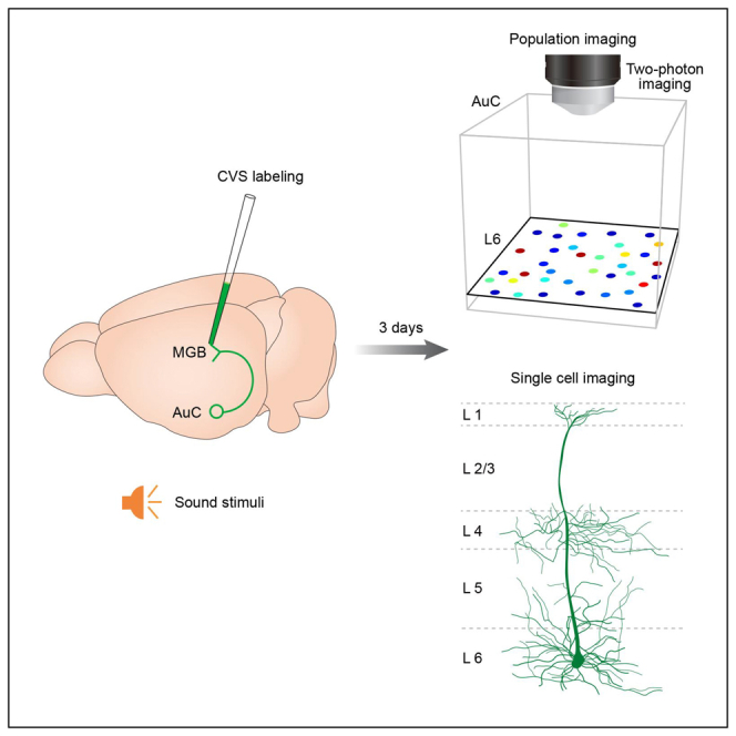
Neocortical layer 6 (L6) is less understood than other more superficial layers, largely owing to limitations of performing high-resolution investigations in vivo. Here, we show that labeling with the Challenge Virus Standard (CVS) rabies virus strain enables high-quality imaging of L6 neurons by conventional two-photon microscopes. CVS virus injection into the medial geniculate body can selectively label L6 neurons in the auditory cortex. Only three days after injection, dendrites and cell bodies of L6 neurons could be imaged across all cortical layers. Ca²⁺ imaging in awake mice showed that sound stimulation evokes neuronal responses from cell bodies with minimal contamination from neuropil signals. In addition, dendritic Ca²⁺ imaging revealed significant responses from spines and trunks across all layers. These results demonstrate a reliable method capable of rapid, high-quality labeling of L6 neurons that can be readily extended to other brain regions.

Graphical abstract

Highlights

• •CVS enables rapid and efficient labeling of L6 CT neurons based on projection specificity
• •CVS enables cellular and subcellular structural imaging of L6 CT neurons
• •CVS enables functional population imaging of L6 CT neurons
• •CVS enables functional single-cell imaging of L6 CT neurons

Optical imaging; Molecular neuroscience; Cellular neuroscience

Introduction

The neocortex is composed of six neuronal layers in mammals.¹ Compared to other layers, L6 is the first to develop but remains relatively understood.^2,3,4 L6 corticothalamic (CT) neurons, as the largest component of the corticofugal projection system, provide CT feedback to the first-order thalamus and send projections to the higher-order thalamus, which integrate many cortical and extracortical synaptic inputs along their dendritic arbors.^5,6,7,8 Although many biomarkers and projections properties of L6 neurons have been revealed, the mechanistic synaptic circuitry underlying information processing in L6 remains obscure, mainly because of the technical difficulties of imaging neurons within deep cortical layers in vivo.^{9,10,11,12,13,14}

Because the initial implementation of two-photon (2P) microscopy in neuroscience, numerous studies of brain function have been performed in mammalian brains at single-cell and subcellular resolution in vivo.^{15,16,17,18,19,20} However, the effective optical penetration depth in practice is primarily restricted to ∼500 μm, reaching, e.g., layer 5a in adult mouse cortex from the pial surface.^21,22,23,24 High-resolution imaging of deeper layers across the whole cortex is technically challenging but essential for understanding the contribution of L6 to brain function and behavior.

To date, there are three main approaches to enable the visualization of deeper brain tissues in vivo while maintaining high optical resolution. First, to replace 2P excitation with three-photon excitation.^25,26 For the same biological fluorophores, the longer wavelength of excitation light can result in less scattering through tissue. Likewise, simply using red-shifted fluorophores can also improve imaging depth.^27,28 Second, to shape the wavefront of excitation light, i.e., use adaptive optics to correct the optical wavefront aberrations induced by brain tissue and thus enable deeper imaging.^29,30 It is also possible to combine these two approaches to further improve the optical penetration depth.^29,31 Third, to remove the excess tissue by surgery and/or to use a prism to convert the side-view along depth to the top-view of microscopy.^32,33 This surgical approach enables unlimited optical access to any arbitrary depth and location in the brain at the cost of invasiveness and tissue damage.

In this study, we present a new approach for deep-layer microscopic imaging in the auditory cortex (AuC) in vivo. It relies primarily on the application of projection-specific retrograde labeling. A CVS strain rabies virus with the glycoprotein gene deleted and pseudotyped with the N2C glycoprotein (CVS-N2c-ΔG) is employed to establish a spatially limited expression profile of L6 CT neurons with significantly improved imaging contrast. The CVS virus is injected into the post-synaptic thalamic region, and thus, the brain tissue beneath the cranial window remains largely intact through the surgery. This method enables the expression of structural indicators (i.e., EGFP) and functional neuronal indicators (e.g., calcium indicators such as GCaMP) in L6 neurons and direct high-quality imaging throughout all the cortical layers with a conventional 2P microscope, without the need for the above-mentioned optical engineering challenges yet still minimizing tissue damage.

Results

Selective labeling of L6 CT neurons with CVS virus

In the AuC, L6 CT projections are sent to the thalamus, with axon collaterals that densely innervate GABAergic neurons in the thalamic reticular nucleus en route to the medial geniculate body (MGB).³⁴ According to a previous study, L6 CT neurons can be subdivided into two morphologically distinct categories: Those with apical dendrites terminating in L4 (32%) and those extending to L1 (68%).³⁵ In this study, an engineered retrograde virus based on the rabies virus CVS-N2c strain was used to attain high-quality structural and functional imaging of AuC L6 CT neurons with a conventional 2P microscope (see STAR Methods for detailed definition).³⁶ CVS-N2c-ΔG-EGFP virus (CVS-EGFP) was injected into the MGB (see STAR Methods for details), which selectively transfected the axon terminals of presynaptic neurons, such as those projecting to the MGB from the AuC (CT neurons, Figure 1A). To determine the injection site, a mixture of CVS-EGFP virus (100 nL, 1.50E+08 titer) and Cholera toxin B conjugated to Alexa 555 (CTB-555) (final concentration, 0.01 mg/mL) was used (Figure 1B). After three days of expression, the labeled cell bodies were observed in deep layers of AuC (Figure 1C). Then, additional immunofluorescence staining of Forkhead box protein P2 (Foxp2) was performed (Figure 1D), which was known as a specific marker for L6 neurons.³⁷ The distances from pia (0 μm) to the upper edge of the Foxp2⁺ and CVS⁺ cells band were measured, respectively (Figure 1E, median/first–third quartile, same notation for all subsequent data. “CVS”: 613.00/600.25–637.25 μm, “Foxp2”: 621.00/572.50–644.50 μm, n = 11 slices from 4 mice). In addition, the thickness of the CVS⁺ neuronal layer was slightly narrower than that of the Foxp2⁺ neuronal layer (Figure 1F, “CVS”: 125.00/121.75–129.00 μm, “Foxp2”: 131.00/127.00–145.75 μm, n = 11 slices from 4 mice, p = 9.77e−04, two-sided Wilcoxon signed-rank test). Co-localization analysis shows that nearly all CVS⁺ neurons exhibited Foxp2⁺ (Figure 1G, “Merge cells”: 98.08/97.88–100.00%, n = 11 slices from 4 mice). And only a tiny fraction of CVS⁺ neurons were found in other layers than L6 (Figure 1H, “L5 cells”: 0.91/0.28–1.43%, n = 13 slices from 4 mice). These results suggest that CVS retrograde labeling selectively labels cell bodies and dendrites, but not axons, of CT neurons in L6 of mouse AuC.

Figure 1.

CVS virus injection in MGB selectively labels cell bodies and dendrites of L6 CT neurons in AuC

(A) Schematic diagram of the injection site of CVS-EGFP in the MGB (Bregma:−3.1 mm).

(B) Coronal slice showing an injection site of CVS-EGFP mixed with CTB-555 in MGB and the retrogradely labeled neurons in the AuC on day 3.

(C) Higher magnification of AuC showing CVS-EGFP labeled neurons.

(D) Foxp2 immunostaining of CVS-labeled section in AuC. White dashed lines show the border of Foxp2.

(E) Boxplots showing the comparison of the distance from pia (0 μm) to the Foxp2-immunopositive neurons and CVS labeled neurons border. n = 11 slices from 4 mice. Median/first – third quartile, same notation for all subsequent data. “CVS”: 613.00/600.25–637.25 μm, “Foxp2”: 621.00/572.50–644.50 μm. p = 0.53, two-sided Wilcoxon signed-rank test.

(F) Boxplots showing the comparison of the distance between the upper and lower edges of the Foxp2-immunopositive or CVS labeled band. n = 11 slices from 4 mice. “CVS”: 125.00/121.75–129.00 μm, “Foxp2”: 131.00/127.00–145.75 μm. p = 9.77e−04, two-sided Wilcoxon signed-rank test.

(G) Boxplot showing the proportions of CVS-labeled neurons expressing Foxp2 in L6. n = 11 slices from 4 mice.

(H) Boxplots showing the fraction of CVS-positive cells in each layer in AuC. n = 13 slices from 4 mice. “L5”: 0.91/0.28–1.43%, “L6”: 99.09/98.57–99.72%.

(I) Coronal slice showing an injection site of retroAAV in MGB and the labeled neurons in the AuC on day 21.

(J) Coronal slice showing an injection site of CTB-488 in MGB and the labeled neurons in the AuC on day 7.

(K) Gray value of CVS, retroAAV, and CTB-488 labeled neurons in AuC with distance from pia (0%) to the L6/WM border (100%).

(L) Boxplots showing the comparison of the gray value of CVS, retroAAV, and CTB-488 labeled neurons in L5 and L6. n = 10 slices taken for each group from 3 mice. L5: “CVS”: 17.00/16.00–18.00, “retroAAV”: 67.50/51.00–78.00, “CTB”: 19.00/15.00–20.00; L6: “CVS”: 79.00/72.00–88.00, “retroAAV”: 8.00/6.00–11.00, “CTB”: 48.00/44.00–49.00. L5: P (retroAAV, CVS) = 1.80e−04, P (retroAAV, CTB) = 1.77e−04, P (CVS, CTB) = 0.24; L6: P (retroAAV, CVS) = 1.76e−04, P (retroAAV, CTB) = 1.72e−04, P (CVS, CTB) = 1.77e−04, two-sided Wilcoxon rank-sum test.

Anatomical studies in various species have indicated that L6 neurons in different primary sensory cortices send feedback projections predominantly to the first-order thalamic nucleus (i.e., ventral MGB of the auditory thalamus, MGBv).^38,39 In contrast, layer 5 (L5) neurons project back to medial and dorsal parts of the thalamic nuclei (i.e., MGBd and MGBm) and other subcortical nuclei.⁴⁰ Considering the labeling discrepancy among different retrograde tracers, we compared the results of CVS labeling with other retrograde labeling methods (retroAAV and CTB, Figures 1I and 1J). Injection of retroAAV in the MGB resulted in labeling predominantly in L5 of AuC (Figure 1I). In contrast, injection of CTB-488 resulted in labeling primarily in L6 (Figure 1J), similar to CVS. To compare the spatial distribution of labeled neurons in different animals, we normalized the cortical thickness of the sections and compared the gray value of the three types of retrogradely labeled cells at 10% bin steps from pia to the L6/white matter border in AuC.⁴¹ Most neurons labeled with retroAAV were found within the neocortex’s 50–80% thickness range, with a dominant peak in the presumptive L5. In contrast, most neurons labeled with CVS virus or CTB-488 were found within the 80–100% thickness range (Figures 1K and 1L). These results were consistent with the previously reported tropism of retrograde tracers within the visual cortex.⁴²

Rapid and effective labeling of L6 CT neurons with CVS virus

To compare the labeling characteristics of the CVS virus with other retrograde tracers, CVS-EGFP, retroAAV, and CTB-488 were injected into the MGB, respectively. CVS-EGFP labeled neurons in AuC were examined on days 1, 2, 3, 7, and 21 (Figure 2A), and the results were compared with those obtained with retroAAV on day 21 (Figure 2B), as well as those obtained with CTB-488 on day 7 (Figure 2C).^43,44 As shown in Figure 2A, green fluorescence (EGPF) from CVS transfection was seen in AuC from day 1, and the fluorescence became more pronounced on day 3. The quantitative analysis showed that the level of EGFP expression was not significantly different on day 3 compared to day 7 or 21 (Figure 2D). Furthermore, the cell numbers and labeling density (labeled cell numbers per unit area) also showed no difference between CVS-labeled neurons on day 3 compared to CTB-488 labeled neurons on day 7 (Figures 2D and 2E). The cell numbers and density of CVS labeling on day 3 were even higher than retroAAV labeling on day 21 (Figures 2D and 2E). These results showed that the CVS virus-based labeling strategy effectively labeled L6 CT neurons in terms of time efficiency compared with retroAAV and CTB: only 3 days are needed for sufficient labeling.

Figure 2.

CVS virus enables rapid and effective labeling of L6 CT neurons

(A) Coronal slice showing the labeled neurons in AuC with CVS-EGFP on days 1, 2, 3, 7,21.

(B) Coronal slice showing the labeled neurons in AuC with retroAAV on day 21.

(C) Coronal slice showing the labeled neurons in AuC with CTB-488 on day 7.

(D) Boxplots showing the comparison of the cell numbers of CVS, retroAAV, and CTB-488 labeled neurons. “CVS 1d”: 37.00/25.00–46.00, n = 13 slices from 3 mice; “CVS 2d”: 89.00/75.00–99.00, n = 13 slices from 3 mice; “CVS 3d”: 160.00/124.00–210.00, n = 13 slices from 3 mice; “CVS 7d”: 171.00/139.00–211.00, n = 12 slices from 3 mice; “CVS 21d”: 177.00/141.00–201.00, n = 12 slices from 3 mice; “CTB 7d”: 194.00/138.00–214.00, n = 11 slices from 3 mice; “retroAAV 21d”: 112.00/107.00–134.00, n = 10 slices from 3 mice. P (CVS 1d, 2d) = 2.58e−05, P (CVS 2d, 3d) = 4.06e−05, P (CVS 3d, 7d) = 0.89, P (CVS 7d, 21d) = 0.91, P (CVS 3d, CTB 7d) = 0.45, P (CVS 3d, retroAAV 21d) = 0.02, two-sided Wilcoxon rank-sum test.

(E) Boxplots showing the comparison of the labeling density of CVS, retroAAV, and CTB-488 labeled neurons. “CVS 1d”: 0.49/0.31–0.57, n = 13 slices from 3 mice; “CVS 2d”: 0.97/0.86–1.10, n = 13 slices from 3 mice; “CVS 3d”: 2.41/1.95–2.76, n = 13 slices from 3 mice; “CVS 7d”: 2.78/2.17–3.15, n = 12 slices from 3 mice; “CVS 21d”: 2.71/2.49–3.10, n = 12 slices from 3 mice; “CTB 7d”: 2.37/2.04–2.66, n = 11 slices from 3 mice; “retroAAV 21d”: 1.48/1.18–1.62, n = 10 slices from 3 mice. P (CVS 1d, 2d) = 3.27e−05, P (CVS 2d, 3d) = 1.65e−05, P (CVS 3d, 7d) = 0.40, P (CVS 7d, 21d) = 0.80, P (CVS 3d, CTB 7d) = 0.74, P (CVS 3d, retroAAV 21d) = 0.06e−02, two-sided Wilcoxon rank-sum test.

Multiscale structural imaging of L6 CT neurons in vivo

To evaluate the CVS labeling capabilities with conventional 2P imaging, we performed structural imaging of L6 CT neurons with CVS or AAV virus in AuC in vivo (see STAR Methods for details). Figure 3A shows a representative z stack of the entire cortical column for CVS virus-labeled CT neurons. The labeled neurons were strong enough in EGFP to enable high-contrast structural imaging throughout all cortical layers. Neuronal dendrites and spines of CVS-labeled neurons had a higher level of EGFP in deeper layers than in AAV-labeled neurons (Figures 3B and 3C). Imaging quality was substantially improved with CVS labeling, as reflected by the much higher signal-to-background ratio, especially at greater tissue depths. Quantitative measurement of the fluorescence intensity profiles of multiscale structures in different layers indicated that CVS labeling resolved single spines down to L5 and dendritic shafts down to L6 (Figures 3D and 3E). Thus, CVS labeling significantly improves the quality of imaging of CT neurons in L6, allowing individual dendrites and spines to be investigated in deeper layers.

Figure 3.

CVS labeling enables multiscale structural imaging of L6 CT neurons in vivo

(A) 3D reconstruction of in vivo imaging of CVS-EGFP labeled neurons on day 3.

(B) Structure imaging of CVS labeled neurons in all layers with CVS-EGFP virus injected into MGB in C57/BL6J mice on day 3.

(C) Structure imaging of AAV labeled neurons in all layers with AAV2/9-hsyn-DIO-EGFP virus injected into AuC in Ntsr1-Cre transgenic mice on day 21.

(D) Relative gray value of CVS and AAV labeled structure along the dashed line in (B) and (C).

(E) Boxplots showing the comparison of the relative gray value of CVS and AAV labeled structure in all layers. n = 10 images taken for each group from 3 mice. L1: “CVS”: 3.30e−04/2.92e−04–3.90e−04, “AAV”: 3.42e−04/3.12e−04–3.72e−04; L2/3: “CVS”: 5.93e−04/5.76e−04–6.10e−04, “AAV”: 3.95e−04/3.60e−04–4.43e−04; L4: “CVS”: 1.97e−04/1.88e−04–2.35e−04, “AAV”: 1.46e−04/0.93e−04–1.91e−04; L5: “CVS”: 2.20e−04/1.93e−04–2.38e−04, “AAV”: 1.15e−04/0.71e−04–1.35e−04; L6: “CVS”: 3.53e−04/3.15e−04–4.00e−04, “AAV”: 1.59e−04/1.48e−04–2.09e−04. P (L1: CVS, AAV) = 0.59, P (L2/3: CVS, AAV) = 1.83e−04, P (L4: CVS, AAV) =0.64e−02, P (L5: CVS, AAV) = 7.69e−04, P (L6: CVS, AAV) = 1.83e−04, two-sided Wilcoxon rank-sum test.

Electrophysiological benchmarking of CVS⁺ and CVS⁻ neurons

To test the robustness of CVS-transfected cells, we performed in vitro patch-clamp recording on both CVS⁺ and CVS⁻ L6 neurons in the AuC. Because the EGFP expression level was insufficient to identify the transfected cells on day 1, we recorded labeled cells from brain slices obtained on day 2 and day 3 (Figures 4A and 4B). No significant difference between the CVS⁺ and nearby CVS⁻ cells were found, including measures of the resting membrane potential (V_m), input resistance (R_in), action potential (AP) peak amplitude, AP rising time, and AP half-width (Figures 4C–4G). In addition, the AP frequency of recorded CVS⁺ neurons exhibited no significant difference compared with CVS⁻ neurons when responding to the current stimulation (Figure 4H), and the current-voltage characteristic (I-V) curve also showed no significant difference (Figure 4I). These results confirm that the CVS-labeled neurons exhibit electrophysiological properties that are indistinguishable from those of normal neurons.

Figure 4.

Electrophysiological benchmarking of CVS⁺ and CVS⁻ neurons

(A) General scheme for whole-cell patch-clamp recording in vitro.

(B) Acute slice for whole-cell patch-clamp recording in vitro. Responses of these cells to injected current pulses (−150, −100, −50, 0, 50, 100, 150, 200 pA) were recorded. 10 neurons were taken for the CVS⁻ group from 5 mice, 8 neurons for the CVS⁺ 2d from 3 mice, and 8 neurons for the CVS⁺ 3d from 3 mice.

(C) Comparison of the resting membrane potential. “CVS^-”:-63.08/-69.26–-58.68, “CVS⁺ 2d”:-66.75/-74.74–-57.84, “CVS⁺ 3d”:-67.50/-69.33–-37.68. P (CVS^-, CVS⁺ 2d) = 0.84, P (CVS^-, CVS⁺ 3d) = 0.33, P (CVS⁺ 2d, CVS⁺ 3d) = 0.37, two-sided Wilcoxon rank-sum test.

(D) Comparison of the input resistance. “CVS^-”: 228.05/184.10–276.50, “CVS⁺ 2d”: 189.85/161.70–217.50, “CVS⁺ 3d”: 144.40/140.63–198.90. P (CVS^-, CVS⁺ 2d) = 0.20, P (CVS^-, CVS⁺ 3d) = 0.07, P (CVS⁺ 2d, CVS⁺ 3d) = 0.37, two-sided Wilcoxon rank-sum test.

(E) Comparison of the AP peak amplitude. “CVS^-”: 58.52/50.41–63.85, “CVS⁺ 2d”: 50.14/37.69–56.68, “CVS⁺ 3d”: 56.84/44.68–71.01. P (CVS^-, CVS⁺ 2d) = 0.07, P (CVS^-, CVS⁺ 3d) = 0.82, P (CVS⁺ 2d, CVS⁺ 3d) = 0.24, two-sided Wilcoxon rank-sum test.

(F) Comparison of the AP rising time. “CVS^-”: 1.76/1.57–2.08, “CVS⁺ 2d”: 1.67/1.47–2.07, “CVS⁺3d”: 1.64/1.51–1.99. P (CVS^-, CVS⁺ 2d) = 0.76, P (CVS^-, CVS⁺ 3d) = 0.74, P (CVS⁺ 2d, CVS⁺ 3d) = 0.99, two-sided Wilcoxon rank-sum test.

(G) Comparison of the AP half-width. “CVS^-”: 2.47/2.00–3.12, “CVS⁺ 2d”: 2.55/1.71–3.18, “CVS⁺ 3d”: 2.02/1.79–2.37. P (CVS^-, CVS⁺ 2d) = 0.81, P (CVS^-, CVS⁺ 3d) = 0.11, P (CVS⁺ 2d, CVS⁺ 3d) = 0.27, two-sided Wilcoxon rank-sum test.

(H) Comparison of the spike frequency. 150pA: “CVS^-”: 1.56/1.25–3.28, “CVS⁺ 2d”: 1.88/0.63–3.13, “CVS⁺ 3d”: 1.56/0.781–2.81; 200pA: “CVS^-”: 2.50/1.72–4.38, “CVS⁺ 2d”: 1.88/0.78–3.75, “CVS⁺ 3d”: 1.88/0.78–4.22. 150pA: P (CVS^-, CVS⁺ 2d) = 0.89, P (CVS^-, CVS⁺ 3d) = 0.64, P (CVS⁺ 2d, CVS⁺ 3d) = 0.64; 200pA: P (CVS^-, CVS⁺ 2d) = 0.55, P (CVS^-, CVS⁺ 3d) = 0.55, P (CVS⁺ 2d, CVS⁺ 3d) = 1.00, two-sided Wilcoxon rank-sum test.

(I) I–V curves of three group data.

Low-contamination Ca²⁺ imaging of L6 CT neuronal populations

We next performed functional imaging of L6 CT neurons in AuC labeled by the CVS-N2c-ΔG-GCaMP6s (CVS-GCaMP6s) virus 3 days after injection in MGB in vivo in awake mice. As expected, the CVS-GCaMP6s virus showed the same tracing retrograde properties as CVS-EGFP (Figures 5A and 5B). One common issue in population Ca²⁺ imaging in vivo was that neuronal signals were often contaminated by the adjacent neuropils.⁴⁵ To ensure that CVS labeling was not prone to such contamination, we randomly sampled the signals of several neurons and their adjacent neuropils (Figures 5C–5E). The amplitude of broadband noise (BBN)-evoked responses from cell bodies were much higher than that from nearby neuropils (Figures 5D and 5E, the amplitude of “Neuron”: 1.38/1.14–1.80, the amplitude of “Neuropil”: 0.13/0.09–0.18, n = 25 neurons from 4 mice, p = 1.22e−05, two-sided Wilcoxon signed-rank test). The data above verified that CVS-GCaMP6s labeling enabled low-contamination Ca²⁺ imaging of CT neurons from L6.

Figure 5.

CVS labeling enables low-contamination Ca²⁺ imaging of L6 CT neuronal populations

(A) Schematic diagram of the injection site of CVS-GCaMP6s in the MGB.

(B) Series slices showing the labeled neurons in AuC from Bregma −2.2 mm to −3.7 mm.

(C) An example of 2P image with CVS-GCaMP6s labeling in vivo. The dashed circles indicate the neurons and neuropils for which Ca²⁺ activity is shown in (D).

(D) BBN-evoked Ca²⁺ signal of neurons and adjacent neuropils in the awake mice. Left: Ca²⁺ activity traces of the example neurons and neuropils (marked in (C)). Right: Data were from 25 neurons and their corresponding 25 adjacent neuropils (4 mice).

(E) Boxplots showing the comparison of the amplitude of neurons and neuropils. n = 25 neurons from 4 mice. “Neuron”: 1.38/1.14–1.80, “Neuropil”: 0.13/0.09–0.18. p = 1.22e−05, two-sided Wilcoxon signed-rank test.

(F) Distribution of the BBN-evoked response in the imaging window of 200 μm × 200 μm (n = 10 focal planes from 4 mice). Each circle represents one neuron. The color code is on the right side of (G).

(G) A pseudo-colored plot summarizing the trial-integrated Ca²⁺ activity trace for each neuron identified as BBN-evoked. n = 897 neurons from 5 mice. Neurons were sorted by their relative increment of activity level (from pre-sound to post-sound). “0” indicated the onset of the BBN stimuli. The color code is on the right side.

(H) Distribution of the success rate for BBN-evoked responses. n = 897 neurons from 5 mice. Neurons defined as “Unreliable” were neurons with a success rate <50% to BBN stimuli, including non-BBN responsive neurons, which showed spontaneous Ca²⁺ transients. The neurons of BBN responses success rate ≥50% were “Reliable.”.

(I) Boxplot showing the percentage of neurons responsive to BBN stimuli in AuC. n = 897 neurons from 5 mice. “Silent neurons”: 38.46/29.08–56.47%, “Unreliable neurons”: 48.00/40.29–60.07%, “Reliable neurons”: 5.71/0.00–16.76%. Neurons were defined as “Silent” when they showed no clear Ca²⁺ transient during the entire recording duration.

Next, we performed functional population imaging of L6 CT neurons labeled by CVS-GCaMP6s in awake mice and calculated the amplitude of each neuron evoked by BBN. Ten focal planes from 4 mice were superimposed to show the characteristics of responses within a window of 200 μm × 200 μm (Figure 5F), and the activity level for all the 897 imaged neurons were sorted by their relative change from pre-sound to post-sound (Figure 5G). We then examined the success rate of BBN-evoked responses, which was defined as the percentage of detectable responses (repetition ≥10). Note that neurons with a success rate <50% to BBN stimuli were defined as “Unreliable” neurons, including those without BBN-evoked responses but with Ca²⁺ transients. The neurons with a success rate ≥50% were defined as “Reliable,” and “Silent” neurons showed no clear Ca²⁺ transients during the entire recording duration (Figure 5H). Here, 5.71/0.00–16.76% of the recorded neurons were “Reliable” neurons, 48.00/40.29–60.07% were “Unreliable” neurons, and 38.46/29.08–56.47% were “Silent” (Figure 5I, n = 897 neurons from 5 mice).

High-quality Ca²⁺ imaging of single-cell subcellular structures across cortical layers

In addition to population imaging, CVS labeling enabled high-quality Ca²⁺ imaging of a single cell at subcellular resolution from superficial to deep cortical layers in the anesthetized mice (Figure 6A). The Ca²⁺ signals of single spines in L1 were easily resolved, with apical trunks in layer 2–5, and cell bodies in L6 (Figure 6A). Ca²⁺ signals from different parts of the same neuron were found from superficial to deep layers (Figures 6C and 6D, n = 7 neurons from 4 mice). However, the amplitude and frequency of Ca²⁺ transients from apical trunks in L4 and L5 were increased considerably compared with superficial layers (Figures 6C and 6D). One neuron was selected to fully reconstruct the functional profile in temporal and spatial dimensions, and a total of 20 focal planes of the neuron were recorded to show the response characteristics of all structures (Figure 6E, from pia to the cell body, 0–608 μm). Together these suggest that by imaging the apical dendrites and somata of L6 CT neurons at single-cell resolution, CVS labeling provides a suitable way to study the ability of dendrites to integrate inputs from spatially isolated pathways.

Figure 6.

CVS labeling enables high-quality Ca²⁺ imaging of single-cell subcellular structures across cortical layers

(A) Reconstruction of a single neuron labeled by the CVS-GCaMP6s virus in all cortical layers.

(B) Left: 2P imaging of a single neuron in all layers with CVS-GCaMP6s. Right: BBN evoked Ca²⁺ signal traces in the anesthetized mice.

(C) Comparison of the Ca²⁺ amplitude in all layers of every single neuron. Ca²⁺ signal response of L1 spine, L2-5 trunk, and L6 cell body. n = 7 neurons from 4 mice. “L1”: 0.00/0.00–0.00, “L2/3”: 0.00/0.00–1.00, “L4”: 1.33/1.14–2.04, “L5”: 2.40/2.02–2.63, “L6”: 0.78/0.60–2.41. P (L2/3, L4) = 0.01, P (L4, L5) = 0.04, two-sided Wilcoxon signed-rank test.

(D) Comparison of the Ca²⁺ frequency in all layers of every single neuron. Ca²⁺ signal response of L1 spine, L2-5 trunk, and L6 cell body. n = 7 neurons from 4 mice. “L1”: 0.00/0.00–0.00, “L2/3”: 0.00/0.00–6.25%, “L4”: 20.00/13.33–37.25%, “L5”: 37.50/34.17–58.37%, “L6”: 50.00/34.17–58.37%. P (L2/3, L4) = 0.20e−02, P (L4, L5) = 0.01, two-sided Wilcoxon signed-rank test.

(E) Front view: A pseudo-colored plot of one single neuron responses to BBN throughout the cortex. Side view: Reconstruction of a single neuron of L6. Top view: Apical dendrites of L6 neuron. The color code is on the right side.

Discussion

In this study, we developed a CVS-based labeling strategy that enables high-contrast, multiscale, structural, and functional imaging of CT neurons in L6 of AuC in mice in vivo.

The CVS-based labeling strategy enables rapid, high-quality imaging of structural and functional details of labeled neurons at large cortical depths. The 2P microscope has been widely used to record neuronal activities within ∼500 μm of mouse cortex.^21,22 Here we present a simple approach to improve the depth penetration using only a conventional 2P microscope. We conducted experiments comparing CVS labeling with AAV labeling (Figure 3). For structural imaging, subcellular profiles of neurons can be obtained after just 3 days of expression whereas other labeling methods usually require more than 1 week (Figure 3A). For functional imaging, high-quality Ca²⁺ imaging of L6 CT neurons can be performed with CVS-GCaMP6s virus by day 3 post-injection (Figures 5F–5I). The high signal-to-background ratio in structural (Figures 3B–3E) and functional (Figures 5C–5E) imaging suggests that the CVS-based labeling strategy is a low-contamination method for in vivo imaging. In addition, CVS is capable of labeling the complete cell morphology at subcellular resolution from spines to cell bodies, thus allowing functional imaging of single-cell subcellular structures (Figure 6). In particular, this strategy provides a suitable approach for studying dendritic integration and characterizing input-output transformations in individual neurons with complex dendritic processes.^2,3

CVS-based labeling primarily relies on the application of projection-specific retrograde labeling. The deep-layer pyramidal neurons are a major source of output from the neocortex.⁸ By exploiting the retrograde nature of rabies virus infection (Figure 1), CVS labeling avoids potential damage to the imaging window because of dye loading/virus injection into the target area, ensuring more excellent stability and consistency in imaging results. In addition, combining CVS with the Cre-loxP recombination system allows both type- and projection-specific neuron labeling.⁴⁶ However, the deep injection required for L6 labeling is accompanied by a higher risk of missing the target site and hitting a blood vessel. It should be noted that labeling selectivity must be carefully assessed before drawing conclusions (see below).

Viruses have emerged as powerful tools for analyzing the structure and function of neural circuits. The CVS-N2c-ΔG rabies virus strain, a recently engineered self-inactivating ΔG rabies virus lacking the polymerase gene, exhibits strong neurotropism. Although our data show no significant differences in electrophysiological properties between CVS⁺ and CVS⁻ neurons (Figure 4), the infection period allowing the most precise imaging should be determined in future work. Previous studies have revealed that reliable neural activity using the CVS-GCaMP6s virus can be maintained for at least 21 days, as recorded by fiber photometry.⁴⁶ In acute forebrain slices, CVS-N2c-ΔG-hChR2-YFP reliably elicits action potentials in transfected cortical neurons for at least 28 days after infection.³⁶ These results suggest that the CVS strain significantly reduced neuronal toxicity compared to the traditional rabies virus. However, it is still unclear if the CVS-based labeling method is suitable for a chronic investigation that lasts for months.

It is long known that different viruses exhibit different infection tropisms in different brain regions.⁴⁷ The distinct tropism of different tracers in the central nervous system may because of the differences in the presence of the corresponding receptors that initiate their entrance into neurons.⁴⁸ Also, host-limiting factors may also repress viral transcription or replication, thus influencing the ultimate efficiency of circuit mapping.⁴⁹ Although the detailed mechanism underlying the selectivity still needs to be further resolved, the labeling preference also enables the investigation of a certain neuronal population. However, it must be kept in mind that, with other labeling methods such as CTB and retroAAV, the specificity of the CVS-based labeling strategy must be double-checked with other methods such as immunofluorescence/in situ hybridization.

Finally, it warrants mention that we used the virus to study the deep layer of AuC, but it has been shown to have similar layer specificity in the visual cortex.⁴² In future studies, it will be interesting to apply this approach to the functional studies of deep layers in other brain regions. The CVS-based labeling approach used in the current work has no additional costs except for the engineered viruses and is thus both affordable and technically tractable for most labs, with fewer surgery-associated risks.⁵⁰ Furthermore, by combining CVS with adaptive optics and/or three-photon imaging, maximum imaging depth can be increased and may eventually be used to detect neuronal network activity in regions previously inaccessible by functional imaging studies in vivo.^26,30

Limitations of the study

This study also has some limitations. For example, it is unclear if the CVS-based labeling method is suitable for a chronic functional study lasting several months. In addition, although we have proved that the method is applicable in AuC, and the layer specificity in the visual cortex has been reported, the applicability to other cortices is still unclear, which still needs further investigations in future studies. At the same time, the functional studies in the AuC L6 of different-projection neuronal subsets are also worth further studies.

STAR★Methods

Key resources table

REAGENT or RESOURCE	SOURCE	IDENTIFIER
Bacterial and virus strains
CVS-N2c-ΔG-EGFP	BrainCase Co., Ltd., Shenzhen, China	BC-RV-N2C862
CVS-N2c-ΔG-GCaM6s	BrainCase Co., Ltd., Shenzhen, China	BC-RV-CVS715
AAV 2/retro-hSyn-EGFP	BrainVTA, China	PT-1990
AAV2/9-hsyn-DIO-EGFP	BrainVTA, China	PT-1103
Antibodies
Goat anti-Foxp2	Abcam	ab1307; RRID: AB_1268914
Alexa Fluor 594-conjugated donkey anti-goat IgG	Invitrogen	A-11058; RRID: AB_142540
Chemicals, peptides, and recombinant proteins
Invitrogen™ Cholera Toxin Subunit B (Recombinant), Alexa Fluor™ 488 Conjugate	Invitrogen	C34775
Invitrogen™ Cholera Toxin Subunit B (Recombinant), Alexa Fluor™ 555 Conjugate	Invitrogen	C34776
DAPI	Sigma-Aldrich	Cat# D9542
Experimental models: organisms/strains
C57BL/6J mouse	Beijing HFK Bioscience Co., Ltd. (China)	https://www.jax.org/; JAX:000664; RRID: IMSR_JAX:000664
Ntsr1-Cre mouse	B6.FVB (Cg)-Tg (Ntsr1-Cre) Gn220Gsat/Mmucd (Jackson Laboratory)	https://www.jax.org/strain/033365

Resource availability

Lead contact

Requests for resources and reagents should be directed to the lead contact Jianxiong Zhang (jianxiong_zhang1988@tmmu.edu.cn).

Materials availability

All the head-fixation apparatus as will be made available on request after completion of a method transfer.

Experimental model and subject details

Animals

C57/BL6J adult (6 to 8 weeks old, male) mice were provided by the Laboratory Animal Center at the Third Military Medical University. B6.FVB (Cg)-Tg (Ntsr1-Cre) Gn220Gsat/Mmucd (Ntsr1-Cre) mice were from the Jackson Laboratory. Mice were housed in groups (5 maximum per cage) under a 12 h light/dark cycle with free access to food and water. All animal procedures were approved by the Animal Care Committee of the Third Military Medical University and were performed in accordance with the principles outlined in the National Institutes of Health Guide for the Care and Use of Laboratory Animals.

Method details

Virus injections, immunofluorescence staining, and confocal imaging

Mice were anesthetized with 1% to 2% isoflurane in pure oxygen and placed in a stereotactic frame (Beijing Zhongshi Dichuang Technology Development Co., Ltd.). A warm heating pad was used to keep the animals at a proper body temperature (36.5°C to 37.5°C). A small craniotomy (0.5 × 0.5 mm) was made above the MGB (AP -3.1 mm, ML 2.0 mm, DV -2.8 mm from dura). Viruses and dyes were used as follows: CVS-N2c-ΔG-EGFP (BC-RV-N2C862) and CVS-N2c-ΔG-GCaM6s (BC-RV-CVS715) were packaged by BrainCase Co., Ltd., Shenzhen, China. The retroAAV-hSyn-EGFP (AAV 2/retro, PT-1990) virus was packaged by BrainVTA. CTB-488 (C34775) and CTB-555 (C34776) were from Invitrogen, Carlsbad, CA, USA. In all the injections, approximately 100 nL of materials were injected into the MGB over ∼5 min. The micropipette was held in place for 10 min before retraction. Tissue glue (3M Animal Care Products, Vetbond) was used for bonding the scalp incision. For slice preparation, mice were perfused transcardially with 4% paraformaldehyde in phosphate-buffered saline. Brains were postfixed in 4% paraformaldehyde overnight at 4°C and cut into 50 μm sections on a cryostat microtome (Thermo Fisher, NX50, Waltham, MA). The Foxp2 immunostaining was performed with the standard protocols. Briefly, a blocking solution was prepared with 5% normal serum (donkey serum, Sigma) and 0.3% Triton-X 100. Selected brain sections were incubated in an appropriate blocking solution at room temperature for 90 min, followed by the application of primary antibodies: goat anti-FOXP2 (1: 500, Abcam, ab1307) for 24 hat 4°C. After washing in PBS, secondary antibodies Alexa Fluor 594-conjugated donkey anti-goat IgG (Invitrogen, A-11058) in the blocking solution was applied at room temperature for 80 min. Mounted sections were imaged on a scanning confocal microscope (TCS SP5, Leica).

Comparative different materials injections, imaging, and quantification

The number of labeled cells per layer was determined by counting the number of EGFP⁺ cells in the tissue slice. Layer boundaries were determined by expert visualization of DAPI labeled nuclei, where available, and pia-WM distance. For the gray value analysis, the distance of CVS, CTB-488, or retroAAV labeled cells present within the region of interest (ROI) was measured from pia to the L6/WM border, and then proportional distance was obtained at 1% steps by normalizing the distance to the cortical thickness with pia and the L6/WM border being 0% and 100%, respectively. The gray value was measured using the Plot Profile (pixel intensity counting) function of Image J. The number of cells at each step was averaged across animals. Cells with a partial structure near the edge of the analysis area were excluded from the analysis.

Two-photon structural imaging

All mice used for structural imaging (Figure 3) were in the anesthetized state. For acute two-photon Ca²⁺ imaging experiments, a cranial window over the right AuC of the mouse was made. In brief, the animal was anesthetized with isoflurane and kept on a heating pad (37.5°C). The skin and muscles over the AuC were removed after local lidocaine injection. A custom-made plastic chamber was glued to the skull with cyanoacrylate glue (UHU), followed by a small craniotomy (∼2 mm × 2 mm) (the center point: Bregma −3.0 mm, 4.5 mm lateral to the midline). To prevent cortical jitter for stable imaging, a piece of glass coverslip was placed on the cranial window and sealed with cyanoacrylate and dental cement.⁵¹ The isoflurane was then reduced to 0.4 – 0.8%, and the animal was transferred to the imaging system.

For CVS labeling (Figures 3A and 3B), mice were used for imaging experiments 3 days after the CVS-EGFP virus was injected into MGB in C57/BL6J mice. Since injection of retroAAV in MGB resulted in labeling predominantly in L5 of AuC (Figure 1I), we performed in vivo structural imaging on the neurons labeled with AAV-DIO-EGFP in adult Ntsr1-Cre mice which specially labeled L6 CT neurons (Figure 3C). Mice were used 21 days after the AAV2/9-hsyn-DIO-EGFP (PT-1103, BrainVTA) virus was injected into AuC (AP -3.1 mm, ML 3.8 mm, angle 20°, DV -1.4 mm from dura) for AAV labeling. The field-of-view (FOV) was chosen some distance away from the area of the brightest EGFP labeling since relative sparseness was useful for substructure identification.

Two-photon imaging was performed with a custom-built 2P microscope system based on a 12.0 kHz resonant scanner (model “LotosScan 1.0”, Suzhou Institute of Biomedical Engineering and Technology). Two-photon excitation light was delivered by a mode-locked Ti: Sa laser (model “Mai-Tai DeepSee,” Spectra-Physics) at a wavelength of 920 nm. A 40×/0.8 NA (Nikon) water-immersion objective was used for imaging, and this objective had a long working distance of 3.5 mm. The typical size of the imaging FOV was ∼200 μm × 200 μm. In a typical experiment, time-lapse imaging recording at different focal depths could be performed sequentially. The average power of the output laser (under the objective) was in the range of 30 – 120 mW, depending on the depth of imaging. For the reconstruction of the neuronal morphology, Z-stack fluorescent images were projected into an averaged image using projection software (Image J). For structural images, the background intensity of each section was subtracted from raw grayscale intensity profiles to minimize the differences.

Two-photon functional imaging

All mice used for population functional imaging (Figure 5) were in the awake state, and for single-cell imaging (Figure 6) were in the anesthetized state. A custom-made plastic chamber (head post) designed for head-fixed mouse experiments was used.⁵² The mouse underwent head-fixation training for 3 days (3h per day). During this training period, the head and the whole body were rotated around 70° based on the craniocaudal axis to keep the surface of AuC perpendicular to the microscope objective. After head-fixation training, mice gradually adapted to this posture and could sit comfortably for 4 h. On the recording day, a small craniotomy (∼2 × 2 mm) was performed on the right AuC after local lidocaine injection under isoflurane anesthesia (1–2%). The recording chamber was perfused with normal artificial cerebral spinal fluid (ACSF) containing 125 mM NaCl, 4.5 mM KCl, 26 mM NaHCO₃, 1.25 mM NaH₂PO₄, 2 mM CaCl₂, 1 mM MgCl₂, and 20 mM glucose (pH 7.4 when bubbled with 95% oxygen and 5% CO₂).

In vitrowhole-cell patch-clamp recording

For brain slice electrophysiology recordings, 11 adult C57/BL6J mice were used. CVS-N2c-ΔG-EGFP was injected into the MGB. After 2 or 3 days, mice were dissected in ice-cold ACSF containing 125 mM NaCl, 2.5 mM KCl, 1.25 mM NaH₂PO₄, 2 mM CaCl₂, 1.3 mM MgSO₄, 26 mM NaHCO₃ and 10 mM glucose, pH 7.4. Coronal sections of 300 μm containing the MGB and AuC were cut using a vibroslicer (752M; Campden Instruments) and recovered in oxygenated ACSF at 35°C for at least 30 min. The slices were then transferred to a submersion-style recording chamber, held in place with a nylon-wired platinum grid, and continuously superfused (4–6ml/min) with oxygenated ACSF at 20 –24°C (room temperature). The membrane voltage was recorded using the whole-cell patch-clamp technique and a MultiClamp 700B patch-clamp amplifier (Molecular Devices). The patch electrodes were pulled from thick-walled borosilicate glass capillaries with resistances of 4 – 7MΩ when filled with an intracellular solution containing 125 mM K⁺-gluconate, 10 mM HEPES, 10 mM EGTA, 4 mM Mg-ATP, 0.3 mM GTP, 2 mM KCl, 0.1 mM CaCl₂, 8 mM phosphocreatine sodium, pH 7.2. The data were obtained at 10 kHz using a Digidata 1322A interface (Molecular Devices) linked to a personal computer controlled by pCLAMP 9.2 (Inchauspe et al. 2012). Recordings were made from visually identified neurons expressing EGFP or no fluorescence. The responses of neurons were observed with injected current pulses (-150, -100, -50, 0, 50, 100, 150, 200 pA). In each slice, multiple neurons were recorded.

Auditory stimulation

The sounds were broadcasted by a free-field ES1 speaker with an ED1 electrostatic speaker driver (Tucker Davis Technologies, USA).⁵³ The broadband noise (BBN, bandwidth 0-50 kHz, duration 50 ms) was generated by a custom-written software based on LabVIEW 2014 (National Instruments, USA) and transduced to an analog voltage by a PCI 6731 card (National Instruments, USA). During experiments, the speaker was put at a distance of ∼6 cm to the left ear of the animal. All sound levels were calibrated with a ¼-inch pressure pre-polarized condenser microphone system (377A01 microphone, 426B03 pre-amplifier, 480E09 signal conditioner, PCB Piezotronics Inc, USA). Data were sampled at 1 MHz via a high-speed data acquisition board USB-6361 from National Instruments and analyzed using custom-written software in LabVIEW 2014. The BBN was applied at ∼a 65 dB sound pressure level (SPL). The background noise (∼55 dB SPL) was below the BBN stimulation level.

Ca²⁺ imaging data analysis

Data were analyzed using custom-written software in LabVIEW 2012 (National Instruments), Igor Pro 5.0 (Wavemetrics), and MATLAB 2014a (MathWorks). To correct motion-related artifacts in imaging data, a frame-by-frame alignment algorithm was used to minimize the sum of squared intensity differences between each frame image and a template, which was the average of the selected image frames. To extract fluorescence signals, neurons were visually identified, and drawing regions of interest (ROIs) based on fluorescence intensity was performed. Fluorescence changes (f) were calculated by averaging the corresponding pixel values for each ROI. Relative fluorescence changes Δf/f = (f−f₀)/f₀ was calculated as Ca²⁺ signals, where the baseline fluorescence f₀ was estimated as the 25th percentile of the entire fluorescence recording. For the Ca²⁺ signals from each neuron recorded in the 2P imaging data, we performed automatic Ca²⁺ transient detection based on thresholding criteria regarding peak amplitude and rising rate.⁵⁴ The noise level was set to be 3 times the standard deviation of the baseline (window length: 1 s). The peak amplitude and the rate of rising of the Ca²⁺ signals were calculated to determine whether it was a true transient. The trace of the detected Ca²⁺ transient was first extracted by exponential infinite impulse response (IIR) filtering (window length: 200 ms) and then subtracted from the original signal. The residual fluorescence trace was used as the baseline for the next transient detection, similar to previously published peeling approaches.⁵⁵

Quantification and statistical analysis

To compare data between groups, we used the nonparametric Wilcoxon rank sum test (unpaired), and Wilcoxon signed-rank test (paired) to determine statistical significance (P < 0.05) between them. In the text, summarized data are presented as the median/ 25th–75th percentiles. In the figures, the data presented in the box-and-whisker plot indicate the median (center line), 25th and 75th percentiles (Q1 and Q3), i.e., interquartile range (IQR) (box), Q1-1.5 × IQR and Q3 + 1.5 × IQR (whiskers), and all other data with error bars are presented as the mean ± s.e.m.

Published: April 8, 2023

Data and code availability

• •The original data reported in this paper is available from the lead contact upon request.
• •This paper does not report original code.
• •Additional information related to this study is available from the lead contact upon request.

References

- 1.Nieuwenhuys R. The neocortex. An overview of its evolutionary development, structural organization and synaptology. Anat. Embryol. 1994;190:307–337. doi: 10.1007/BF00187291. [DOI] [PubMed] [Google Scholar]
- 2.Chen X., Leischner U., Rochefort N.L., Nelken I., Konnerth A. Functional mapping of single spines in cortical neurons in vivo. Nature. 2011;475:501–505. doi: 10.1038/nature10193. [DOI] [PubMed] [Google Scholar]
- 3.Jia H., Rochefort N.L., Chen X., Konnerth A. Dendritic organization of sensory input to cortical neurons in vivo. Nature. 2010;464:1307–1312. doi: 10.1038/nature08947. [DOI] [PubMed] [Google Scholar]
- 4.Abdel-Mannan O., Cheung A.F.P., Molnár Z. Evolution of cortical neurogenesis. Brain Res. Bull. 2008;75:398–404. doi: 10.1016/j.brainresbull.2007.10.047. [DOI] [PubMed] [Google Scholar]
- 5.Zhang Z.W., Deschênes M. Intracortical axonal projections of lamina VI cells of the primary somatosensory cortex in the rat: a single-cell labeling study. J. Neurosci. 1997;17:6365–6379. doi: 10.1523/JNEUROSCI.17-16-06365.1997. [DOI] [PMC free article] [PubMed] [Google Scholar]
- 6.Kumar P., Ohana O. Inter- and intralaminar subcircuits of excitatory and inhibitory neurons in layer 6a of the rat barrel cortex. J. Neurophysiol. 2008;100:1909–1922. doi: 10.1152/jn.90684.2008. [DOI] [PubMed] [Google Scholar]
- 7.Kirchgessner M.A., Franklin A.D., Callaway E.M. Context-dependent and dynamic functional influence of corticothalamic pathways to first- and higher-order visual thalamus. Proc. Natl. Acad. Sci. USA. 2020;117:13066–13077. doi: 10.1073/pnas.2002080117. [DOI] [PMC free article] [PubMed] [Google Scholar]
- 8.Baker A., Kalmbach B., Morishima M., Kim J., Juavinett A., Li N., Dembrow N. Specialized subpopulations of deep-layer pyramidal neurons in the neocortex: bridging cellular properties to functional consequences. J. Neurosci. 2018;38:5441–5455. doi: 10.1523/JNEUROSCI.0150-18.2018. [DOI] [PMC free article] [PubMed] [Google Scholar]
- 9.Heavner W.E., Ji S., Notwell J.H., Dyer E.S., Tseng A.M., Birgmeier J., Yoo B., Bejerano G., McConnell S.K. Transcription factor expression defines subclasses of developing projection neurons highly similar to single-cell RNA-seq subtypes. Proc. Natl. Acad. Sci. USA. 2020;117:25074–25084. doi: 10.1073/pnas.2008013117. [DOI] [PMC free article] [PubMed] [Google Scholar]
- 10.Marin I.A., Gutman-Wei A.Y., Chew K.S., Raissi A.J., Djurisic M., Shatz C.J. The nonclassical MHC class I Qa-1 expressed in layer 6 neurons regulates activity-dependent plasticity via microglial CD94/NKG2 in the cortex. Proc. Natl. Acad. Sci. USA. 2022;119 doi: 10.1073/pnas.2203965119. e2203965119. [DOI] [PMC free article] [PubMed] [Google Scholar]
- 11.Takeuchi A., O'Leary D.D.M. Radial migration of superficial layer cortical neurons controlled by novel Ig cell adhesion molecule MDGA1. J. Neurosci. 2006;26:4460–4464. doi: 10.1523/JNEUROSCI.4935-05.2006. [DOI] [PMC free article] [PubMed] [Google Scholar]
- 12.Galazo M.J., Emsley J.G., Macklis J.D. Corticothalamic projection neuron development beyond subtype specification: Fog2 and intersectional controls regulate intraclass neuronal diversity. Neuron. 2016;91:90–106. doi: 10.1016/j.neuron.2016.05.024. [DOI] [PMC free article] [PubMed] [Google Scholar]
- 13.Molyneaux B.J., Arlotta P., Menezes J.R.L., Macklis J.D. Neuronal subtype specification in the cerebral cortex. Nat. Rev. Neurosci. 2007;8:427–437. doi: 10.1038/nrn2151. [DOI] [PubMed] [Google Scholar]
- 14.Zhou Y., Liu B.H., Wu G.K., Kim Y.J., Xiao Z., Tao H.W., Zhang L.I. Preceding inhibition silences layer 6 neurons in auditory cortex. Neuron. 2010;65:706–717. doi: 10.1016/j.neuron.2010.02.021. [DOI] [PMC free article] [PubMed] [Google Scholar]
- 15.Svoboda K., Denk W., Kleinfeld D., Tank D.W. In vivo dendritic calcium dynamics in neocortical pyramidal neurons. Nature. 1997;385:161–165. doi: 10.1038/385161a0. [DOI] [PubMed] [Google Scholar]
- 16.Svoboda K., Helmchen F., Denk W., Tank D.W. Spread of dendritic excitation in layer 2/3 pyramidal neurons in rat barrel cortex in vivo. Nat. Neurosci. 1999;2:65–73. doi: 10.1038/4569. [DOI] [PubMed] [Google Scholar]
- 17.Brustein E., Marandi N., Kovalchuk Y., Drapeau P., Konnerth A. "In vivo" monitoring of neuronal network activity in zebrafish by two-photon Ca(2+) imaging. Pflugers Arch. 2003;446:766–773. doi: 10.1007/s00424-003-1138-4. [DOI] [PubMed] [Google Scholar]
- 18.Seelig J.D., Chiappe M.E., Lott G.K., Dutta A., Osborne J.E., Reiser M.B., Jayaraman V. Two-photon calcium imaging from head-fixed Drosophila during optomotor walking behavior. Nat. Methods. 2010;7:535–540. doi: 10.1038/nmeth.1468. [DOI] [PMC free article] [PubMed] [Google Scholar]
- 19.Helmchen F., Svoboda K., Denk W., Tank D.W. In vivo dendritic calcium dynamics in deep-layer cortical pyramidal neurons. Nat. Neurosci. 1999;2:989–996. doi: 10.1038/14788. [DOI] [PubMed] [Google Scholar]
- 20.Varga Z., Jia H., Sakmann B., Konnerth A. Dendritic coding of multiple sensory inputs in single cortical neurons in vivo. Proc. Natl. Acad. Sci. USA. 2011;108:15420–15425. doi: 10.1073/pnas.1112355108. [DOI] [PMC free article] [PubMed] [Google Scholar]
- 21.Oheim M., Beaurepaire E., Chaigneau E., Mertz J., Charpak S. Two-photon microscopy in brain tissue: parameters influencing the imaging depth. J. Neurosci. Methods. 2001;111:29–37. doi: 10.1016/s0165-0270(01)00438-1. [DOI] [PubMed] [Google Scholar]
- 22.Takasaki K., Abbasi-Asl R., Waters J. Superficial bound of the depth limit of two-photon imaging in mouse brain. eNeuro. 2020;7 doi: 10.1523/ENEURO.0255-19.2019. ENEURO.0255-19.2019. [DOI] [PMC free article] [PubMed] [Google Scholar]
- 23.Hill D.N., Varga Z., Jia H., Sakmann B., Konnerth A. Multibranch activity in basal and tuft dendrites during firing of layer 5 cortical neurons in vivo. Proc. Natl. Acad. Sci. USA. 2013;110:13618–13623. doi: 10.1073/pnas.1312599110. [DOI] [PMC free article] [PubMed] [Google Scholar]
- 24.Kondo S., Yoshida T., Ohki K. Mixed functional microarchitectures for orientation selectivity in the mouse primary visual cortex. Nat. Commun. 2016;7:13210. doi: 10.1038/ncomms13210. [DOI] [PMC free article] [PubMed] [Google Scholar]
- 25.Kobat D., Durst M.E., Nishimura N., Wong A.W., Schaffer C.B., Xu C. Deep tissue multiphoton microscopy using longer wavelength excitation. Opt Express. 2009;17:13354–13364. doi: 10.1364/Oe.17.013354. [DOI] [PubMed] [Google Scholar]
- 26.Ouzounov D.G., Wang T., Wang M., Feng D.D., Horton N.G., Cruz-Hernández J.C., Cheng Y.T., Reimer J., Tolias A.S., Nishimura N., Xu C. In vivo three-photon imaging of activity of GCaMP6-labeled neurons deep in intact mouse brain. Nat. Methods. 2017;14:388–390. doi: 10.1038/nmeth.4183. [DOI] [PMC free article] [PubMed] [Google Scholar]
- 27.Dana H., Mohar B., Sun Y., Narayan S., Gordus A., Hasseman J.P., Tsegaye G., Holt G.T., Hu A., Walpita D., et al. Sensitive red protein calcium indicators for imaging neural activity. Elife. 2016;5:e12727. doi: 10.7554/eLife.12727. [DOI] [PMC free article] [PubMed] [Google Scholar]
- 28.Tischbirek C.H., Birkner A., Konnerth A. In vivo deep two-photon imaging of neural circuits with the fluorescent Ca(2+) indicator Cal-590. J. Physiol. 2017;595:3097–3105. doi: 10.1113/JP272790. [DOI] [PMC free article] [PubMed] [Google Scholar]
- 29.Tang J., Germain R.N., Cui M. Superpenetration optical microscopy by iterative multiphoton adaptive compensation technique. Proc. Natl. Acad. Sci. USA. 2012;109:8434–8439. doi: 10.1073/pnas.1119590109. [DOI] [PMC free article] [PubMed] [Google Scholar]
- 30.Ji N. Adaptive optical fluorescence microscopy. Nat. Methods. 2017;14:374–380. doi: 10.1038/nmeth.4218. [DOI] [PubMed] [Google Scholar]
- 31.Qin Z., She Z., Chen C., Wu W., Lau J.K.Y., Ip N.Y., Qu J.Y. Deep tissue multi-photon imaging using adaptive optics with direct focus sensing and shaping. Nat. Biotechnol. 2022;40:1663–1671. doi: 10.1038/s41587-022-01343-w. [DOI] [PubMed] [Google Scholar]
- 32.Kaifosh P., Lovett-Barron M., Turi G.F., Reardon T.R., Losonczy A. Septo-hippocampal GABAergic signaling across multiple modalities in awake mice. Nat. Neurosci. 2013;16:1182–1184. doi: 10.1038/nn.3482. [DOI] [PubMed] [Google Scholar]
- 33.Lovett-Barron M., Kaifosh P., Kheirbek M.A., Danielson N., Zaremba J.D., Reardon T.R., Turi G.F., Hen R., Zemelman B.V., Losonczy A. Dendritic inhibition in the hippocampus supports fear learning. Science. 2014;343:857–863. doi: 10.1126/science.1247485. [DOI] [PMC free article] [PubMed] [Google Scholar]
- 34.Guo W., Clause A.R., Barth-Maron A., Polley D.B. A corticothalamic circuit for dynamic switching between feature detection and discrimination. Neuron. 2017;95:180–194.e5. doi: 10.1016/j.neuron.2017.05.019. [DOI] [PMC free article] [PubMed] [Google Scholar]
- 35.Olsen S.R., Bortone D.S., Adesnik H., Scanziani M. Gain control by layer six in cortical circuits of vision. Nature. 2012;483:47–52. doi: 10.1038/nature10835. [DOI] [PMC free article] [PubMed] [Google Scholar]
- 36.Reardon T.R., Murray A.J., Turi G.F., Wirblich C., Croce K.R., Schnell M.J., Jessell T.M., Losonczy A. Rabies virus CVS-N2c(DeltaG) strain enhances retrograde synaptic transfer and neuronal viability. Neuron. 2016;89:711–724. doi: 10.1016/j.neuron.2016.01.004. [DOI] [PMC free article] [PubMed] [Google Scholar]
- 37.Clayton K.K., Williamson R.S., Hancock K.E., Tasaka G.I., Mizrahi A., Hackett T.A., Polley D.B. Auditory corticothalamic neurons are recruited by motor preparatory inputs. Curr. Biol. 2021;31:310–321.e5. doi: 10.1016/j.cub.2020.10.027. [DOI] [PMC free article] [PubMed] [Google Scholar]
- 38.Ojima H. Terminal morphology and distribution of corticothalamic fibers originating from layers 5 and 6 of cat primary auditory cortex. Cereb. Cortex. 1994;4:646–663. doi: 10.1093/cercor/4.6.646. [DOI] [PubMed] [Google Scholar]
- 39.Llano D.A., Sherman S.M. Evidence for nonreciprocal organization of the mouse auditory thalamocortical-corticothalamic projection systems. J. Comp. Neurol. 2008;507:1209–1227. doi: 10.1002/cne.21602. [DOI] [PubMed] [Google Scholar]
- 40.Takayanagi M., Ojima H. Microtopography of the dual corticothalamic projections originating from domains along the frequency axis of the cat primary auditory cortex. Neuroscience. 2006;142:769–780. doi: 10.1016/j.neuroscience.2006.06.048. [DOI] [PubMed] [Google Scholar]
- 41.Chang M., Kawai H.D. A characterization of laminar architecture in mouse primary auditory cortex. Brain Struct. Funct. 2018;223:4187–4209. doi: 10.1007/s00429-018-1744-8. [DOI] [PubMed] [Google Scholar]
- 42.Sun L., Tang Y., Yan K., Yu J., Zou Y., Xu W., Xiao K., Zhang Z., Li W., Wu B., et al. Differences in neurotropism and neurotoxicity among retrograde viral tracers. Mol. Neurodegener. 2019;14:8. doi: 10.1186/s13024-019-0308-6. [DOI] [PMC free article] [PubMed] [Google Scholar]
- 43.Tervo D.G.R., Hwang B.Y., Viswanathan S., Gaj T., Lavzin M., Ritola K.D., Lindo S., Michael S., Kuleshova E., Ojala D., et al. A designer AAV variant permits efficient retrograde access to projection neurons. Neuron. 2016;92:372–382. doi: 10.1016/j.neuron.2016.09.021. [DOI] [PMC free article] [PubMed] [Google Scholar]
- 44.Cui J.J., Wang J., Xu D.S., Wu S., Guo Y.T., Su Y.X., Liu Y.H., Wang Y.Q., Jing X.H., Bai W.Z. Alexa Fluor 488-conjugated cholera toxin subunit B optimally labels neurons 3-7 days after injection into the rat gastrocnemius muscle. Neural Regen. Res. 2022;17:2316–2320. doi: 10.4103/1673-5374.337055. [DOI] [PMC free article] [PubMed] [Google Scholar]
- 45.Garaschuk O., Milos R.I., Konnerth A. Targeted bulk-loading of fluorescent indicators for two-photon brain imaging in vivo. Nat. Protoc. 2006;1:380–386. doi: 10.1038/nprot.2006.58. [DOI] [PubMed] [Google Scholar]
- 46.Lin K.Z., Li L., Ma W.Y., Yang X., Han Z.P., Luo N.S., Wang J., Xu F.Q. A rabies virus-based toolkit for efficient retrograde labeling and monosynaptic tracing. Neural Regen. Res. 2023;18:1827–1833. doi: 10.4103/1673-5374.358618. [DOI] [PMC free article] [PubMed] [Google Scholar]
- 47.Zhu X., Lin K., Liu Q., Yue X., Mi H., Huang X., He X., Wu R., Zheng D., Wei D., et al. Rabies virus pseudotyped with CVS-N2C glycoprotein as a powerful tool for retrograde neuronal network tracing. Neurosci. Bull. 2020;36:202–216. doi: 10.1007/s12264-019-00423-3. [DOI] [PMC free article] [PubMed] [Google Scholar]
- 48.Li S.J., Vaughan A., Sturgill J.F., Kepecs A. A viral receptor complementation strategy to overcome CAV-2 tropism for efficient retrograde targeting of neurons. Neuron. 2018;98:905–917.e5. doi: 10.1016/j.neuron.2018.05.028. [DOI] [PubMed] [Google Scholar]
- 49.Albisetti G.W., Ghanem A., Foster E., Conzelmann K.K., Zeilhofer H.U., Wildner H. Identification of two classes of somatosensory neurons that display resistance to retrograde infection by rabies virus. J. Neurosci. 2017;37:10358–10371. doi: 10.1523/JNEUROSCI.1277-17.2017. [DOI] [PMC free article] [PubMed] [Google Scholar]
- 50.Zheng Y., Chen J., Shi X., Zhu X., Wang J., Huang L., Si K., Sheppard C.J.R., Gong W. Two-photon focal modulation microscopy for high-resolution imaging in deep tissue. J Biophotonics. 2019;12:e201800247. doi: 10.1002/jbio.201800247. [DOI] [PubMed] [Google Scholar]
- 51.Zhao C., Chen S., Zhang L., Zhang D., Wu R., Hu Y., Zeng F., Li Y., Wu D., Yu F., et al. Miniature three-photon microscopy maximized for scattered fluorescence collection. Nat. Methods. 2023 doi: 10.1038/s41592-023-01777-3. [DOI] [PubMed] [Google Scholar]
- 52.Li J., Liao X., Zhang J., Wang M., Yang N., Zhang J., Lv G., Li H., Lu J., Ding R., et al. Primary auditory cortex is required for anticipatory motor response. Cereb Cortex. 2017;27:3254–3271. doi: 10.1093/cercor/bhx079. [DOI] [PubMed] [Google Scholar]
- 53.Zhang J., He Y., Liang S., Liao X., Li T., Qiao Z., Chang C., Jia H., Chen X. Non-invasive, opsin-free mid-infrared modulation activates cortical neurons and accelerates associative learning. Nat. Commun. 2021;12:2730. doi: 10.1038/s41467-021-23025-y. [DOI] [PMC free article] [PubMed] [Google Scholar]
- 54.Li J., Zhang J., Wang M., Pan J., Chen X., Liao X. Functional imaging of neuronal activity of auditory cortex by using Cal-520 in anesthetized and awake mice. Biomed. Opt Express. 2017;8:2599–2610. doi: 10.1364/boe.8.002599. [DOI] [PMC free article] [PubMed] [Google Scholar]
- 55.Grewe B.F., Langer D., Kasper H., Kampa B.M., Helmchen F. High-speed in vivo calcium imaging reveals neuronal network activity with near-millisecond precision. Nat. Methods. 2010;7:399–405. doi: 10.1038/nmeth.1453. [DOI] [PubMed] [Google Scholar]
Associated Data
This section collects any data citations, data availability statements, or supplementary materials included in this article.
Supplementary Materials
Data Availability Statement