Different approaches to explore the impact of COVID-19 lockdowns on carbonaceous aerosols at a European rural background site

Abstract

To prevent the fast spread of COVID-19, worldwide restrictions have been put in place, leading to a reduction in emissions from most anthropogenic sources. In this study, the impact of COVID-19 lockdowns on elemental (EC) and organic (OC) carbon was explored at a European rural background site combining different approaches: − “Horizontal approach (HA)” consists of comparing concentrations of pollutants measured at 4 m a.g.l. during pre-COVID period (2017–2019) to those measured during COVID period (2020-2021); − “Vertical approach (VA)” consists of inspecting the relationship between OC and EC measured at 4 m and those on top (230 m) of a 250 m-tall tower in Czech Republic. The HA showed that the lockdowns did not systematically result in lower concentrations of both carbonaceous fractions unlike NO₂ (25 to 36 % lower) and SO₂ (10 to 45 % lower). EC was generally lower during the lockdowns (up to 35 %), likely attributed to the traffic restrictions whereas increased OC (up to 50 %) could be attributed to enhanced emissions from the domestic heating and biomass burning during this stay-home period, but also to the enhanced concentration of SOC (up to 98 %). EC and OC were generally higher at 4 m suggesting a greater influence of local sources near the surface. Interestingly, the VA revealed a significantly enhanced correlation between EC and OC measured at 4 m and those at 230 m (R values up to 0.88 and 0.70 during lockdown 1 and 2, respectively), suggesting a stronger influence of aged and long distance transported aerosols during the lockdowns. This study reveals that lockdowns did not necessarily affect aerosol absolute concentrations but it certainly influenced their vertical distribution. Therefore, analyzing the vertical distribution can allow a better characterization of aerosol properties and sources at rural background sites, especially during a period of significantly reduced human activities.

Graphical abstract

1. Introduction

Atmospheric carbonaceous aerosols, including particulate elemental (EC) and organic carbon (OC), are one of the key components of ambient aerosols (Putaud et al., 2004) attracting increasing interest due to their adverse effects on human health, atmospheric visibility, and climate forcing (Andreae and Ramanathan, 2013; Bond et al., 2013; IPCC, 2013). EC is a surrogate for black carbon (BC), considered the dominant aerosol light absorber playing a major role in altering the Earth's radiation budget (Andreae and Ramanathan, 2013; Bond et al., 2013). OC is predominantly a light scatterer; only a fraction of OC called brown carbon (BrC) contributes to light absorption (Andreae and Gelencsér, 2006; Bond et al., 2013; Feng et al., 2013; Kirchstetter et al., 2004). Aside from emission sources, several meteorological parameters can influence ambient aerosol concentrations. The structure and dynamics of the planetary boundary layer (PBL), the part of the troposphere closest to the Earth's surface influenced by interaction with it (up to 2 km high), are key factors strongly influencing air pollution (Stull, 1988; Tang et al., 2016). The mixing layer height (MLH), a measure of the vertical turbulent exchange within the PBL, determines the concentrations of atmospheric air pollutants in the near-surface layer as well as their dispersion, transport, reaction, and settling (Geiß et al., 2017; Kanawade et al., 2019; Srivastava et al., 2014).

Analyzing the vertical distribution of atmospheric aerosols with respect to the evolution of PBL is important to better describe the effect of aerosols on human health, characterize local and regional emission sources, understand fog, haze and smog formation, and also evaluate regional climate forcing (Altstädter et al., 2020; Singh et al., 2018). However, there is a limited amount of in-situ measurement data dealing with the vertical distributions of carbonaceous aerosol, and this is especially true in Europe. Meteorological tall-tower platforms offer the possibility of long-term, continuous measurements of aerosol vertical gradient. However, there are only a few tall-tower experimental setups, often not more than a hundred meters tall, and studies have been conducted for a relatively short period of time (Choomanee et al., 2020; Li et al., 2020a; Sun et al., 2020).

The novel Coronavirus Disease 2019 (COVID-19) emerged in China in late 2019 and became a worldwide outbreak by early 2020. Globally, as of July 2022, WHO recorded over 546 million confirmed cases of COVID-19 including over 6 million deaths (WHO, 2022). Over 228 million confirmed cases were reported in Europe including over 2 million deaths. In Czechia, from January 2020 to July 2022, there have been over 3 million confirmed cases with over 40,000 deaths (https://COVID19.who.int/). Like in many countries, a series of both preventive and control measures limiting human activities had been implemented by the Czech authorities to prevent COVID-19 from spreading quickly. In Czech Republic, two city lockdowns were implemented (lockdown 1: from March 14 to May 18, 2020, lockdown 2: October 5, 2020, to April 11, 2021) with restrictions on traffic and most economic and social activities (Fig. 1 ).

Fig. 1.

Number of COVID_19 daily new cases and lockdowns (red areas) in Czech Republic. Numbers in the first lockdown are in the inset plot for better readability. Data of COVID daily cases (WHO, 2022).

The stay-home policies during the COVID-19 lockdowns resulted in a significant reduction of emissions of air pollutants from most kinds of anthropogenic sources such as traffic, industry, and institutional and commercial buildings. As a result, several studies, mostly conducted in urban areas, have reported a decrease in air pollutants concentrations: Brazil (Dantas et al., 2020); China (Bhatti et al., 2022; Meng et al., 2021; Xie et al., 2022); India (Rajesh and Ramachandran, 2022; Sharma et al., 2020); Italy (Collivignarelli et al., 2020); Morocco (Otmani et al., 2020); Spain (Baldasano, 2020; Clemente et al., 2022); USA (Antony Chen et al., 2020; Hudda et al., 2020; Zangari et al., 2020). Aside from this, the stay-home policies during the lockdowns could also lead to increased emissions from domestic activities (i.e. biomass burning) which could counterbalance the reduced emissions from other anthropogenic sources such as traffic (Altuwayjiri et al., 2021; Sicard et al., 2020). Despite the large number of studies on the effect of COVID-19 lockdowns on air quality, few have been conducted in rural environments. To the best of our knowledge, no study has observed an effect of lockdowns on vertical aerosol mixing.

The COVID-19 pandemic is an unprecedented occasion to characterize the properties of atmospheric aerosols at a rural background site during periods with drastically reduced emissions from numerous types of human activities. This study aims to investigate the impact of COVID-19 lockdowns on carbonaceous aerosols at a European rural background combining different approaches based on continuous in-situ measurements of vertical distribution. Due to a limited number of tall-tower atmospheric observational platforms, this study will ostensibly be the first of its kind worldwide.

2. Material and methods

2.1. Monitoring site

The National Atmospheric Observatory Košetice (NAOK, 49°35′N, 15°05′E; 534 m a.s.l.) is a Central European rural background site involved in numerous European monitoring and research programs (Cavalli et al., 2016; Schwarz et al., 2016). The site is located in an agricultural landscape in the Bohemian-Moravian Highlands around 70 km SE of the city of Prague (population of 1,300,000, CSO, 2021), Czech Republic (Fig. 2 ). One of the main Czech highways (40,756 cars/day, CSD, 2016) is approximately 6 km north and northeast. NAOK is affected by regional and long-distance transported air masses, mainly associated with western and southeastern winds (Dvorská et al., 2015; Mbengue et al., 2018, Mbengue et al., 2020, Mbengue et al., 2021; Schwarz et al., 2016; Vodička et al., 2015).

Fig. 2.

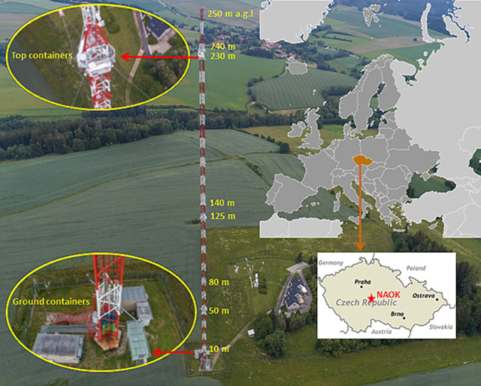
Geographical location of the National Atmospheric Observatory Košetice (NAOK) and photographs of the tall tower with sampling containers at ground level and on top (230 m).

The station provides a unique infrastructure in Central Europe, consisting of sampling containers at the foot of a tall tower with measurement platforms at different elevations (Fig. 2). It was designed and equipped exclusively for scientific purposes according to recommendations by ICOS (Integrated Carbon Observation System), ACTRIS (Aerosol, Clouds, Trace Gases Research Infrastructure Network), GMOS (Global Mercury Observation System), and AERONET (AErosol RObotic NETwork). The tall tower consists of a 250-m tall lattice guyed mast of a 2.6 m wide triangular lattice structure, allowing for good ventilation and minimizing airflow disturbances.

2.2. Carbonaceous aerosol measurements

Ground-based (4 m a.g.l.) long-term monitoring of EC and OC has been carried out at the NAOK since 2013 using a semi-continuous thermal-optical OCEC analyzer (Sunset Laboratory Inc., USA) placed in a measurement container at the foot of the tall tower (Fig. 2). Part of this work has previously been published (Mbengue et al., 2018, Mbengue et al., 2020, Mbengue et al., 2021; Schwarz et al., 2016; Vodička et al., 2015). In late 2019, a second OCEC analyzer was placed in a sampling container on top of the tower (230 m a.g.l) and measurements were performed simultaneously with ground measurements from December 2019 to June 2021. During the campaign, a total of 2553 and 2504 samples were collected at ground level and on top of the tall-tower respectively, including 1955 pairs of OCEC data points.

Airborne particles were sampled at a flow rate of 8.0 l min⁻¹ with a PM_2.5 cyclone inlet placed at 4 m and 230 m a.g.l. To accumulate enough material on the sampling quartz fiber filter, both instruments sampled with a 4 h time resolution (2:00, 6:00, 10:00, 14:00, 18:00 and 22:00, UTC) including 20 min of OCEC thermo-optical analysis according to the shortened EUSAAR-2 protocol (Cavalli et al., 2010; Karanasiou et al., 2020). The OCEC thermo-optical protocol is described in Supplementary materials (Appendix A, Table S1). The sampling systems were equipped with a carbon parallel-plate diffusion denuder (Sunset Laboratory Inc., USA) to prevent positive artifacts induced by the absorption of volatile organic compounds on the quartz fiber filter (Turpin et al., 2000). According to Arhami et al. (2006), the positive artefact that could make up over 50 % of measured OC was practically eliminated using a denuder. To check the stability of the instrument, blanks (0 min sampling) were measured once daily at 2:00 and control calibrations using standard sucrose solutions were performed twice a month at ground level and monthly on top of the tower. The denuders for removing volatile organic compounds in the gas phase were changed at three-month intervals in both cases.

EC is a primary pollutant emitted directly into the air during combustion processes of carbonaceous material (Bond and Bergstrom, 2006). OC can be emitted by anthropogenic or biogenic sources as primary organic carbon (POC) while secondary organic carbon (SOC) can also be formed in the atmosphere from the oxidation of reactive organic gases and gas-to-particle conversion processes (Kim et al., 2000; Schwarz et al., 2008). The contribution of secondary organic carbon (SOC) to the total OC concentration was estimated as the difference between OC and the primary organic carbon (POC) using the EC tracer method (Mbengue et al., 2018; Pio et al., 2011; Wu and Yu, 2016):

$$\mathrm{OC}=\mathrm{POC}+\mathrm{SOC}$$ (1)

$$\mathrm{POC}={\left[\mathrm{OC}/\mathrm{EC}\right]}_{\mathrm{pri}}\times \mathrm{EC}$$ (2)

The EC tracer method has an advantage in simplicity and low cost. However, the determination of the primary OC/EC ratio ([OC/EC]_pri) is a crucial point as it could be affected by primary emissions from biomass burning, especially during the colder seasons (Mbengue et al., 2018; Pio et al., 2011). In this study, the [OC/EC]_pri was estimated by applying the minimum R squared (MRS) using EC and OC as input variables (Wu and Yu, 2016; Wu et al., 2018). The Igor Pro-based computer program (WaveMetrics, Inc. Lake Oswego, OR, USA) built by Wu (2017) was used for the MRS estimation of [OC/EC]_pri and SOC. The correlation (R²) between measured EC and estimated SOC was investigated assuming a series of hypothetical [OC/EC]_pri values varying from 0.1 to 10. Considering the independence between EC and SOC, the minimum R² (between EC and SOC) would correspond to the best [OC/EC]_pri of the data set.

2.3. Other air pollutants

The NAOK is part of the Czech air quality monitoring network operated by the Czech Hydrometeorological Institute (CHMI). Long-term continuous measurements of gaseous pollutants such as NO₂ and NO_x (chemiluminescence), SO₂ (UV-photometric), CO (IR abs. spectrometry), particulate matter (aerodynamic diameters ≤10 μm (PM₁₀) and ≤ 2.5 μm (PM_2.5), radiometry and beta-ray absorption) are performed hourly at ground level by the CHMI (Mbengue et al., 2018, Mbengue et al., 2020).

2.4. Meteorological data and atmospheric dispersion

Meteorological parameters such as temperature (T), relative humidity (RH), wind speed (WS) and direction (WD) were monitored at different heights of the tower by the Global Change Research Institute (CzechGlobe, The Czech Academy of Sciences).

A ceilometer Vaisala CL51 (Vaisala Inc., Finland) placed on the ground near the tower was used to observe the characteristics of the MLH. This device is based on LIDAR (Light Detection And Ranging) technology and the process of measuring backscatter profiles data using BL-VIEW software. Output from BL-VIEW was consequently evaluated by the method published by Lotteraner and Piringer (2016) to determine the PBL height.

The ventilation coefficient (VC) is a good proxy to understand the accumulation and dispersion efficiency of air pollutants within the PBL (Ashrafi et al., 2009; Dai et al., 2020; Tiwari et al., 2016). It is defined as the potential volume into which air pollutants are diluted per unit of time and can be calculated as the product of the MLH (vertical dilution of pollutants: m) and the mean wind speed (horizontal ventilation: m s⁻¹) (Dai et al., 2020; Tiwari et al., 2016):

$$\mathrm{VC}=\mathrm{MLH}\times {\mathrm{WS}}_{\mathrm{mean}}$$ (3)

In theory, higher VC leads to cleaner air. In this study, the VC was calculated for different seasons, and the mean wind speed (WS_mean) was obtained using measurement data recorded at five altitudes alongside the tower.

2.5. OC and EC source areas

The conditional bivariate probability function (CBPF) and potential source contribution function (PSCF) analyses were used to explore the contribution of the geographical origins of sources affecting the NAOK receptor site at different altitudes.

The CBPF analysis (Uria-Tellaetxe and Carslaw, 2014) was performed for OC and EC at ground level and on top of the tower using the openair package (Carslaw and Ropkins, 2012) in R (R Core Team, 2020) and the 75^th percentile was used as a threshold, i.e., the probability of the concentration being between the 75^th and 100^th percentiles was calculated for each wind speed and direction recorded at 10 m and 230 m a.g.l, respectively.

The PSCF calculation was also performed at ground level and on top of the tower using the split and openair R packages. The analysis was performed with 72-h air mass back trajectories (AMBT) arriving at 50 m and 230 m a.g.l., respectively. The AMBTs were calculated every 6 h using the HYSPLIT_4 model and meteorological data from the Global Data Assimilation System (GDAS) archive information with a resolution of 1° × 1° (Rolph et al., 2017; Stein et al., 2015). Details regarding the CBPF and PSCF can be found in our previous studies (Mbengue et al., 2020, Mbengue et al., 2021; Zíková et al., 2016).

3. Results and discussion

3.1. Overview of carbonaceous aerosol vertical distribution

The temporal patterns of the EC and OC measured at 4 m and 230 m a.g.l. of the tall tower from December 2019 to June 2021 are presented in Fig. 3 , along with trace gaseous pollutants, particulate matter and meteorological parameters. A seasonal variation was observed for EC and OC measured at 4 m a.g.l., with higher values in winter and lower in summer (Table 1 and Fig. 3a and b). This is more pronounced for EC, with winter/summer ratio of 2.32 compared to OC (1.36). SOC showed an opposite pattern with higher concentration in summer (winter/summer ratio of 0.73), which in turn, led to an increased SOC/OC ratio (64 ± 11 %). NO_x, SO₂, CO, displayed comparable seasonal patterns with winter/summer ratios of 2.01, 1.38 and 1.15, respectively (Fig. 3c). For particulate matter (Fig. 3d), the seasonal variation is more pronounced for PM_2.5 (winter/summer ratio of 1.25) compared to PM₁₀ (winter/summer ratio of 1.08). The higher concentration in winter could be attributed to greater emissions from combustion sources combined with the lower and more stable MLH observed during this season (Fig. 3e). The latter leads to a worsening of atmospheric horizontal and vertical dispersion, resulting in an accumulation of pollutants in a thin layer above the surface (Ashrafi et al., 2009; Dai et al., 2020; Tiwari et al., 2016).

Fig. 3.

Time series of monthly mean concentrations of carbonaceous aerosols, trace gaseous pollutants, PM_2.5 and PM₁₀, and meteorological parameters measured at different heights (4 m and 230 m a.g.l.) from December 2019 to June 2021. The arrows in (e) indicate the average wind directions for each month.

Table 1.

Concentration means ± standard deviations of EC, OC and SOC measured at 4 m and 230 m a.g.l., and their 4 m/230 m ratios during the observation period from December 2019 to June 2021.

		EC (μg m−3)	OC (μg m−3)	SOC (μg m−3), SOC/OC (%)
Whole period	4 m	0.39 ± 0.33	3.16 ± 2.02	1.49 ± 1.13, 47 ± 20
	230 m	0.25 ± 0.33	1.50 ± 1.18	0.58 ± 0.53, 38 ± 20
	4 m/230 m	1.48	2.05	2.57
2020	4 m	0.34 ± 0.29	2.72 ± 1.75	1.29 ± 0.93, 47 ± 20
	230 m	0.23 ± 0.29	1.44 ± 1.09	0.60 ± 0.50, 39 ± 20
	4 m/230 m	1.47	1.89	2.15
Winter	4 m	0.51 ± 0.38	3.36 ± 2.33	1.27 ± 1.27, 36 ± 20
	230 m	0.31 ± 0.45	1.44 ± 1.34	0.40 ± 0.45, 29 ± 16
	4 m/230 m	1.76	2.46	3.18
Spring	4 m	0.41 ± 0.33	3.29 ± 2.05	1.50 ± 1.15, 45 ± 19
	230 m	0.27 ± 0.26	1.62 ± 1.12	0.57 ± 0.42, 37 ± 17
	4 m/230 m	1.43	1.93	2.63
Summer	4 m	0.21 ± 0.11	2.74 ± 1.31	1.74 ± 0.84, 64 ± 11
	230 m	0.14 ± 0.22	1.56 ± 1.17	1.12 ± 0.62, 62 ± 14
	4 m/230 m	1.29	1.49	1.55
Autumn	4 m	0.34 ± 0.24	3.05 ± 1.86	1.61 ± 0.99, 53 ± 15
	230 m	0.20 ± 0.15	1.33 ± 0.88	0.53 ± 0.49, 37 ± 17
	4 m/230 m	1.67	2.36	3.04

At 230 m a.g.l., EC showed a similar behaviour as observed at ground level with a winter/summer ratio of 1.71, whereas OC showed an opposite behaviour with slightly higher values in spring and summer when the concentration of O₃ was higher (Fig. 3d). On top of the tower, the winter/summer ratio for OC was 0.83. This could be associated with the enhanced contribution of SOC in summer (Fig. 4a, Table 1), which was more pronounced at 230 m where a lower winter/summer ratio (0.36) was observed for SOC, compared to the ground level. On the upper part of the tower, SOC likely associated with aged aerosols seems to offset the weaker influence of local primary sources on OC concentration.

Fig. 4.

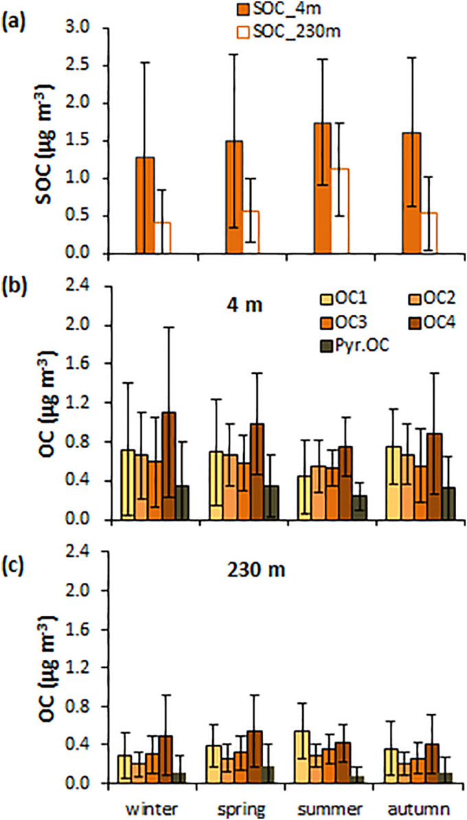
Seasonal mean concentrations of SOC (a) and OC sub-fractions measured from December 2019 to June 2021 at 4 m (b) and 230 m a.g.l. (c). Whiskers are standard deviations.

During the observation period, the correlation between OC and EC was also higher at 4 m than at 230 m a.g.l., with correlation coefficients (R) of 0.81 and 0.66, respectively. Seasonally, R values were comparable at ground level (from 0.81 to 0.83) while at the top they varied from 0.35 in summer to 0.79 in autumn. These results suggest the influence of different emission sources and/or different meteorological conditions at the different sampling heights.

The concentrations of carbonaceous aerosols were generally higher at ground level with the ground/top ratio (ratio between concentration at 4 m and 230 m) of 1.48 for EC, 2.05 for OC and 2.57 for SOC (Table 1). This ratio ranged from 1.29 and 1.49 in summer to 1.76 and 2.46 in winter for EC and OC, respectively. For SOC, the 4 m/230 m ratio was 1.55 in summer and 3.18 in winter. The larger difference observed between concentrations at ground level and on top of the tower during colder seasons, and especially in winter, suggests a larger influence of local primary combustion sources at 4 m, especially during this season. This is likely associated with the emissions from residential biomass burning, which form the abundant fraction of organic compounds (Mbengue et al., 2020; Sandradewi et al., 2008) consistent with the higher 4 m/230 m ratios observed for OC and SOC compared to EC. The weaker correlation between OC and EC and the stronger wind observed at 230 m (Fig. 3e) suggest a larger influence of aged, mixed, and long range transported aerosols at this altitude. This is confirmed by the CBPF analysis at both heights (Fig. 5 ). During the campaign, EC, OC, and SOC measured at ground level showed a higher probability of exceeding the 75^th percentile of values under low wind speed conditions (5 m s^{− 1}) around the sampling site, indicating that they were likely influenced by local sources. Conversely, at 230 m, higher OC and EC levels were observed under stronger wind speeds (> 10 m s⁻¹) from the south-east, whereas higher SOC levels were associated with low to moderate wind speeds. Although the prevalent wind directions observed at 4 m and 230 m were mostly similar, the higher wind speeds observed on top of the tower could promote the dilution of aerosols of local origin, and conversely transport long distance pollutants to the receptor site.

Fig. 5.

CBPF polar plots of the probability of EC and OC exceeding the 75th percentile of concentrations in relation to wind direction and wind speed at the NAOK.

In addition to the OC, we analysed four OC sub-fractions depending on their volatility (from OC1 — most volatile to OC4 — least volatile) and the pyrolytic carbon (PC) part. The mean concentrations of different OC sub-fractions measured at 4 m and 230 m a.g.l. are depicted in Fig. 4, and their contributions to total OC (%) are shown in Fig. S1. At 4 m, all OC sub-fractions and PC showed a similar seasonal pattern as OC with higher values in winter and lower in summer (Fig. 4b). OC4 was generally predominant (24-28 %), followed by OC1 accounting for 18 % (winter) to 22 % (autumn) at 4 m. The prevalence of OC4 was previously observed at the NAOK by Vodička et al. (2015) using the same analytical protocol which shows that this is a long-term phenomenon. Higher contributions of less volatile OC were also observed in rural and remote sites (Pio et al., 2007; Zhu et al., 2014), whereas the prevalence of PC was observed in different urban (Sillanpää et al., 2005; Zhu et al., 2014) and rural/background sites in Europe (Pio et al., 2007). In the present study, PC showed the lowest concentrations at both heights during all seasons, accounting for 8 % - 9 % at 4 m and 3 % - 7 % at 230 m. The most volatile OC sub-fractions and PC have been attributed to fresh aerosol, sourced from fossil fuel combustion (Sahu et al., 2011) as well as coal and/or biomass combustion in urban areas (Vodička et al., 2015).

At 230 m, OC1, OC2 and OC3 showed opposite behaviour with higher values in summer while OC4 and PC displayed similar seasonal behaviour as observed at 4 m (Fig. 4c). On top of the tower, the increase of the most volatile OC sub-fractions in summer is more pronounced for OC1, which was the prevalent OC sub-fraction (29 %), while OC4 was predominant during other seasons (24 % - 28 %) similar to that at ground level. Among all sub-fractions, only OC1 showed a higher concentration at 230 m (0.54 μg m⁻³) in summer compared to 4 m (0.44 μg m⁻³), and its prevalence during this season could be attributed to increasing SOC which showed a similar seasonal pattern (Ehn et al., 2014). Furthermore, the correlation between SOC and OC1 was stronger at 230 m (R = 0.80) than at 4 m (R = 0.69).

3.2. Influence of COVID 19 restrictions on carbonaceous aerosols

Two approaches were used in this study to explore the impact of COVID-19 at the rural site. The first approach, which will be referred to as the “horizontal approach (HA)”, consists of a comparison of concentrations of selected pollutants measured at ground level during the pre-COVID period (2017–2019) to those measured during the COVID period (2020-2021) considering different time scales (annual, seasonal, and diurnal). The second approach is named the “vertical approach (VA)”; it entails the inspection of the relationship between OC and EC measured at 4 m and that measured at 230 m a.g.l. of a tall tower.

3.2.1. Inter-annual variability

The annual mean concentrations of OC, EC, trace gaseous pollutants, PM_2.5, and PM₁₀ measured at ground level in 2020 are compared to those recorded during the pre-COVID years 2017–2019 (Fig. 6 ). Annual mean EC concentrations measured in 2020 (0.34 ± 0.29 μg m^{− 3}) were 38 % lower than preceding years. The contribution of EC to PM_2.5 mass decreased over the years reaching its lowest value (3.8 %) in 2020 compared to pre-COVID periods (Fig. 6a). For OC, its concentration decreased by 18 % in 2020 compared to the pre-COVID period (3.31 ± 2.13 μg m^{− 3}), and no decrease was observed for the OC/PM_2.5 ratio over 2017–2020 (Fig. 6b).

Fig. 6.

Annual mean concentrations of a) EC, b) OC, c) particulate matter, and e) and f) trace gaseous pollutants measured at 4 m a.g.l. during pre-COVID (from 2017 to 2019) and COVID years (2020) in bars. The diamonds in a) and b) show EC/PM_2.5 and OC/PM_2.5 ratios. d) shows the amount of rain and number of rainy days per year defined as a day with at least 1 mm of rain in 24 h. Whiskers are standard deviations.

EC is a primary pollutant emitted predominantly from combustion sources. Therefore, a decrease in its concentration could be expected during the COVID period as a consequence of traffic restrictions during the lockdown. During the period 2017–2020, EC, PM₁₀ and PM_2.5 (Fig. 6a and 6c) showed similar trends, with their highest levels being observed in 2018, which could be explained by the less abundant rain recorded during this year (Fig. 6d). PM₁₀ and PM_2.5 were around 20 % lower in 2020 compared to the overall mean concentration during the period 2017–2019. Although the concentration of CO was slightly higher in 2018, it was around 7.2 % lower in 2020 compared to the pre-COVID period. Unlike aerosol particles, NO_x, NO₂, and SO₂ showed their highest levels in 2017 and a decreasing trend during the following years, with concentrations 32 % lower in 2020 compared to the pre-COVID period (Fig. 6f). No clear pattern for O₃ was observed over the measurement period (Fig. 6f).

3.2.2. Seasonal variation during normal and COVID periods

During the campaign, the implementation of the first lockdown on March 14^th, 2020, coincided with the decreasing concentration from spring to summer, whereas the start of the second lockdown on October 5^th, 2020, coincided with the increasing concentration from autumn to winter (Fig. 3). Therefore, there is no perceptible drop in OC and EC concentrations due to the lockdowns in Fig. 3. To examine the impact of COVID restrictions, the concentrations of OC and EC measured at ground level during the pre-COVID period (from 2017 to 2019) were compared to the values recorded during 2020–2021 as a whole for different seasons, and those measured during the two controlled periods for corresponding seasons (Fig. 7 ). When there was no lockdown in the Czech Republic in summer 2020, no effect was expected.

Fig. 7.

Seasonal mean concentrations of EC (a), OC (b), and SOC (c) measured at 4 m a.g.l. during pre-COVID (from 2017 to 2019) and COVID periods. The COVID period includes the two individual lockdowns and the entirety of 2020–2021 with lockdowns. Whiskers are standard deviations.

In addition to source emission rates during different seasons, the concentration of ambient pollutants can be influenced by the meteorology. Meteorological normalization techniques have been used to decouple the effects of meteorological factors (Dai et al., 2020; Grange et al., 2018; Lin et al., 2021; Petetin et al., 2020; Shi et al., 2021). In this study, dispersion normalized concentrations have been calculated using the ventilation coefficient to reduce the effects of meteorologically induced dilution during the pre-COVID and COVID periods (Dai et al., 2020):

$$\mathrm{nX}=\mathrm{Xi}\times \frac{{\mathrm{VC}}_{\mathrm{i}}}{{\mathrm{VC}}_{\text{mean}}}$$ (4)

where $\mathit{nX}$is dispersion normalized concentration of pollutant X, $\mathit{Xi}$ is its concentration measured during period i, and ${\mathit{VC}}_i$ is the ventilation coefficient during period i, and ${\mathit{VC}}_{\mathit{mean}}$ is its average value over the whole sampling period; these were 2682 m² s⁻¹ and 2282 m² s⁻¹ for the pre-COVID and COVID periods, respectively.

The levels of EC measured during the pre-COVID period were 36 %, 16 %, and 34 % higher than those overall observed during 2020–2021 for winter (0.51 μg m⁻³), spring (0.43 μg m⁻³), and autumn (0.35 μg m⁻³), respectively (Fig. 7a). The normalized EC concentration (nEC) showed comparable results with 25 %, 9 %, and 45 % lower concentrations during the 2020–2021 for winter, spring, and autumn, respectively (Fig. S2a). EC concentrations recorded during lockdown 1 were 10 % lower than those recorded pre-COVID for the same season (0.51 μg m⁻³) whereas nEC was 3 % higher. During lockdown 2, EC observed during winter and autumn were 35 % and 25 % lower than those measured pre-COVID (0.80 μg m⁻³ and 0.53 μg m⁻³, respectively), whereas there was no difference in spring 2021. nEC was 28 %, 11 % and 46 % lower during winter, spring, and autumn, respectively.

As for OC, there was different behaviour compared to EC (Fig. 7b). The OC level was 17 % lower in winter 2020–2021 compared to the pre-COVID period while it was 3 % and 10 % higher in spring and autumn, respectively. nOC was 3 % and 10 % higher in winter and spring, respectively, and 2 % lower in autumn (Fig. S2b). The OC level recorded during the first lockdown was 12 % lower than that recorded pre-COVID whereas during the second lockdown, it increased by 50 % and 28 % in spring and autumn, respectively, in comparison to the pre-COVID period (3.17 μg m⁻³ and 2.86 μg m⁻³, respectively). Similarly to OC, nOC was 11 % lower during lockdown 1 and showed increased values during lockdown 2 by 19 %, 45 % and 5 % in winter, spring and autumn, respectively. The increasing concentration of OC during the second lockdown could be related to a larger influence of emissions from the local domestic activities (e.g. residential heating, biomass burning) during this stay-home period (Altuwayjiri et al., 2021; Sicard et al., 2020). During the lockdown 2, increased OC was also associated with an enhanced concentration of SOC at 4 m (Fig. 7c) which resulted in a higher SOC/OC ratio (Fig. 3b). During colder seasons, the higher SOC/OC ratio observed at 4 m (up to 60 %) could be related to the influence of local biomass burning. SOC was 56 %, 98 %, and 95 % higher than those observed pre-COVID for winter (1.45 μg m⁻³), spring (1.55 μg m⁻³), and autumn (1.20 μg m⁻³), respectively. nSOC showed a similar pattern during lockdown 2, when it was 51 %, 44 %, and 42 % higher for winter, spring, and autumn, respectively (Fig. S2c). Enhanced formation of secondary aerosols has been observed during the lockdown in urban areas, attributed to a reduction of NO_x and PM concentrations and an increase in O_3, which in turn, can lead to an enhanced oxidizing capacity of the atmosphere (Clappier et al., 2021; Feng et al., 2022; Meng et al., 2021). In this study, SOC showed an opposite pattern compared to O₃, which was 5 % higher during lockdown 1 and 15 % to 27 % lower during lockdown 2 (Fig. S3). This result can potentially be related to different chemical processes controlling secondary aerosol formations in respect to primary emissions in rural areas compared to urban environments, such as where emissions of traffic related NO₂ could be more important during normal periods.

During the campaign, both measured and normalized concentrations of NO₂, SO₂, PM₁₀, and PM_2.5 displayed lower levels during the COVID period regardless of season (Fig. S3, Fig. S4), showing similar behaviour as EC, except in spring. The drop in concentration during the lockdown periods was more prominent for NO₂ (nNO₂), and SO₂ (nSO₂) which are directly influenced by anthropogenic sources - around 36 % (43 %) and 45 % (47 %), respectively during lockdown 1, and by 28 % to 37 % (38 to 49 %) for NO₂ and by 10 % to 38 % (2 to 57 %) for SO₂ during lockdown 2. As most economic activities were restricted, the reduced concentration of primary pollutants (EC) and short-lived trace gas species (NO₂, and SO₂) during the controlled periods could be attributed to lower emissions of anthropogenic origin, such as traffic and industrial activities. Similar behaviours were also observed in different urban areas (Li et al., 2020b; Meng et al., 2021; Xu et al., 2020).

3.2.3. Diurnal variation of EC and OC at different altitudes

The diurnal cycles of EC and OC measured at 4 m and 230 m a.g.l. are plotted for different seasons during the COVID period (2020-2021) at different heights in comparison to the pre-COVID period (from 2017 to 2019) at ground level (Fig. 8 ). The diurnal patterns of carbonaceous aerosols measured at 4 m during the pre-COVID period, and especially so for EC, were similar to those previously observed at the NAOK during 2013–2016 (Mbengue et al., 2018) with maximums during the morning traffic rush hour (between 6:00 and 10:00) and in the evening (between 18:00 and 22:00). During the campaign, comparable diurnal patterns were also observed at ground level for NO_x, SO₂ (Fig. S5), displaying a bimodal distribution. The highest levels of OC and EC were observed during the evening, which could be attributed to poor atmospheric dilution due to low and stable MLH (Fig. S6) and the concomitant influence of traffic and domestic activities, e.g. local residential biomass burning, particularly in winter (Mbengue et al., 2018, Mbengue et al., 2020, Mbengue et al., 2021). EC and OC reached minima in the noon/afternoon when the MLH and VC are at their maximum height (Fig. S6).

Fig. 8.

Mean diurnal variations of EC and OC for different seasons during the pre-COVID (from 2017 to 2019 at 4 m) and COVID (2020-2021) periods at 4 m a.g.l. (a and b) and at 230 m a.g.l. (c and d). COVID period includes the two individual lockdowns and the entirety 2020–2021 with lockdowns.

During COVID periods, the morning EC peak seemed less visible at 4 m (Fig. 8a), and especially in spring and autumn, likely due to the traffic restrictions in place during the lockdown periods. Comparable diurnal behaviour was observed for NO_x and SO₂ (Fig. S5). During lockdown 2, OC at 4 m showed increasing concentration during the daytime (Fig. 8b), possibly related to increased emissions from residential heating and biomass burning (Altuwayjiri et al., 2021; Sicard et al., 2020). At 230 m, EC and OC both generally displayed opposite behaviour from that observed at ground level (Fig. 8c and 8d), with maximum levels around noon/afternoon having similar diurnal profiles to those of the MLH and VC (Fig. S6). With the increased MLH height at noontime, pollutants confined to a thin layer above the ground during night time and early morning could be diluted (high VC) and transported up to higher altitude (Lu et al., 2019).

3.2.4. Relationship between OC and EC at different heights

As indicated in the previous sections, the restrictions during the COVID lockdowns did not always result in decreased concentrations of carbonaceous aerosols. This was especially the case during the second lockdown for EC in spring and for OC in all seasons. Inspecting the relationship between carbonaceous fractions measured at different heights could provide insight regarding the potential sources, composition, and transformation of atmospheric aerosols.

During pre-lockdown 1 (December 2019 to February 2020), a weak correlation (R ≤ 0.24) was observed between EC measured at 4 m and that at 230 m (Fig. 9a). The correlation steeply increased (up to 0.88) in March 2020, when lockdown 1 was implemented, and dropped once again in June after the first control period. There was again an enhanced correlation during lockdown 2 starting in October 2020 with R values up to 0.70 in February 2021. OC seemed to exhibit similar behaviours during both lockdowns. The enhanced correlation observed during the lockdowns, particularly for EC, a primary pollutant, suggests that the aerosols collected at 4 m and 230 m a.g.l. were influenced by common sources and/or transported simultaneously at the sampling site during those periods. The COVID restrictions may result in reduced emissions from most human activities such as traffic and industries. Consequently, there may well be a smaller influence of local sources at the receptor site and a higher contribution of aged and long-distance transported aerosols. In addition to the lockdown periods, OC also showed an enhanced correlation in summer, likely associated with SOC formation consistent with the elevated SOC/OC ratio observed during this season (Fig. 3 and 4, and Table 1).

Fig. 9.

(a) Time series of monthly correlation coefficients between EC and OC at 4 m and 230 m from December 2019 to June 2021; (b, c, d, and e) PSCF of the EC sources calculated separately for different seasons during lockdowns at ground level and top of the tower with the seasonal 75th percentile as the limit value. The location of NAOK is denoted by a black circle.

The potential source contribution function (PSCF) analysis was performed during the lockdowns to identify potential source regions of EC collected at 4 m and 230 m of the tower over different seasons (Fig. 9). During lockdown 1, PSCF results show similar source locations at both heights, with the most probable sources of EC being located in southern Poland and the western regions of Slovakia and Ukraine (Fig. 9b). This is consistent with the strong relationship (R = 0.88) observed during this period between EC at 4 m and 230 m, although the PSCF plot shows a more extensive source region for EC on the top. During lockdown 2 in autumn 2020, the potential sources of EC were observed from the south with a higher probability observed from northern Italy for the ground and from the southeast (Balkan regions) for the top (Fig. 9c). This difference could explain the slightly lower correlation (R = 0.51) observed in autumn between EC at 4 m and 230 m compared to the remaining period of lockdown 2 (Fig. 9d and 9e). Indeed, during winter 2020–21 (R = 0.61) and spring 2021 (R = 0.62), the PSCF analysis revealed similar sources regions for EC at both heights with the most probable sources of EC being located in eastern Czech Republic, the south (Silesia region) and western Poland.

The results of this study show that the lockdown clearly influence the vertical distribution of carbonaceous aerosols. Therefore, analyzing vertical distributions provides important insights useful for better examining the impact of COVID lockdowns at rural sites far from abundant anthropogenic sources.

4. Summary and conclusion

In this study, the vertical distribution of carbonaceous aerosols and the impact of the COVID-19 lockdowns have been investigated at a Czech rural site representing background air pollution in Central Europe. Ground-based (4 m a.g.l.) and tall tower (230 m a.g.l.) measurements of OC and EC were characterized in relation to their potential sources and the evolution of the PBL. The concentrations of OC and EC were higher at 4 m height more influenced by emissions from local sources, whereas measurements on top of the tower could be more affected by aged, well-mixed, and long-range transported aerosols. EC at both elevations and OC on the ground showed seasonal patterns similar to those observed for the short-lived trace gases (NO₂, NO_x and SO₂); these showed higher values in winter, possibly associated with larger emissions from combustion sources during this season. OC measured at 230 m showed the opposite behaviour with slightly higher values during warmer seasons, related to the enhanced contribution of secondary organic carbon (SOC), more pronounced on top of the tower where it increased by 134 % in summer relative to the value observed in winter. In general, opposite diurnal profiles were observed for the different heights. The highest levels of OC and EC were observed at ground level during the evening, while there was a lower and more stable MLH. In contrast, increased concentrations were observed on top of the tower, associated with the enhanced atmospheric dispersion of pollutants (higher VC) at noon due to the developed MLH.

To analyze the effect of the lockdown restrictions imposed by authorities to reduce the spread of COVID-19, two approaches (HA and VA) have been applied based on in-situ measurements of vertical distribution. To reduce the effects of meteorological conditions, dispersion normalized concentrations have been calculated during the pre-COVID and COVID periods. The HA showed that the restrictions during the COVID lockdowns did not necessarily lead to lower concentration of all carbonaceous fractions at the rural background site, unlike NO₂, NO_x and SO₂ which are directly influenced by anthropogenic sources. Generally EC and nEC showed lower concentrations (up to 35 % and 46 %, respectively) during the lockdowns which could be attributed to traffic restrictions, whereas increased OC and nOC, especially during lockdown 2 (50 %), could be attributed to enhanced emissions from the domestic activities (e.g. residential heating, biomass burning) during this stay-home period, but also to the enhanced concentration of SOC and nSOC (up to 98 % and 51 %, respectively). The COVID lockdowns effect was better observed using the VA which examines the correlation of EC and OC between 4 m and 230 m. Indeed, due to the reduced emission from local anthropogenic sources during the controlled period, aerosols measured at 4 m seemed to be more associated with aged aerosols transported over long distances, leading to stronger correlations between measures at ground level and on the top of the tower.

This study reveals that lockdowns did not systematically affect aerosol absolute concentrations but it certainly influenced their vertical distribution. Therefore surveying solely the concentrations of carbonaceous aerosols at ground level may not be efficient for clearly observing particular events (e.g. the impact of COVID lockdowns) at a rural background environment. Supplementary measures at different heights are necessary for this purpose. Further studies dealing with the vertical distribution of aerosols extended to other physicochemical properties should be conducted in order to better understand the uncertainties related to radiative forcing and human health.

CRediT authorship contribution statement

Saliou Mbengue: Conceptualization and design of the project, Field measurements, Data curation, Formal analysis, Visualization, and Interpretation of results, and Writing – original draft preparation. Petr Vodička: Conceptualization, Critical discussions, Review, and Editing. Kateřina Komínková: Data collection, curation, and Analysis of the meteorological data, Critical discussions, Review and Editing. Nadežda Zíková: Source apportionment analysis, Visualization and Interpretation of data, Critical discussions, Review, and Editing. Jaroslav Schwarz: Critical discussions, Review and Editing. Roman Prokeš: Supervision, Critical discussions, Review and Editing. Lenka Suchánková: Field measurements, Data Analysis, Critical discussions, Review and Editing. Kajal Julaha: Critical discussions, Review and Editing. Jakub Ondráček, Ivan Holoubek, and Vladimír Ždímal: Funding acquisition, Project administration and Supervision, Review and Editing. The authors read and approved the final manuscript.

Declaration of competing interest

The authors declare no conflict of interest.

Editor: Jianmin Chen

Appendix A. Supplementary data

Supplementary material

Data availability

OC and EC data measured at 4 m a.g.l. can be downloaded from the EBAS database (http://ebas.nilu.no/). The data measured at 230 m a.g.l. are available from the corresponding authors upon request.

References

- Altstädter B., Deetz K., Vogel B., Babic K., Dione C., Pacifico F., Jambert C., Ebus F., Bärfuss K., Pätzold F., Lampert A., Adler B., Kalthoff N., Lohou F. The vertical variability of black carbon observed in the atmospheric boundary layer during DACCIWA. Atmos. Chem. Phys. 2020;20:7911–7928. [Google Scholar]
- Altuwayjiri A., Soleimanian E., Moroni S., Palomba P., Borgini A., Marco C.D., Ruprecht A.A., Siouta C. The impact of stay-home policies during Coronavirus-19 pandemic on the chemical and toxicological characteristics of ambient PM2.5 in the metropolitan area of Milan, Italy. Sci. Total Environ. 2021;758 doi: 10.1016/j.scitotenv.2020.143582. [DOI] [PMC free article] [PubMed] [Google Scholar]
- Andreae M.O., Gelencsér A. Black carbon or brown carbon? The nature of light-absorbing carbonaceous aerosols. Atmos. Chem. Phys. 2006;6:3131–3148. [Google Scholar]
- Andreae M.O., Ramanathan V. Climate's dark forcings. Science. 2013;340:280–281. doi: 10.1126/science.1235731. [DOI] [PubMed] [Google Scholar]
- Antony Chen L.-W., Chien L.C., Li Yi, Lin G. Nonuniform impacts of COVID-19 lockdown on air quality over the United States. Sci. Total Environ. 2020;745 doi: 10.1016/j.scitotenv.2020.141105. [DOI] [PMC free article] [PubMed] [Google Scholar]
- Arhami M., Kuhn T., Fine P.M., Delfino R.J., Sioutas C. Effects of sampling artifacts and operating parameters on the performance of a semicontinuous particulate elemental carbon/organic carbon monitor. Environ. Sci. Technol. 2006;40:945–954. doi: 10.1021/es0510313. [DOI] [PubMed] [Google Scholar]
- Ashrafi K., Shafie-Pour M., Kamalan H. Estimating temporal and seasonal variation of ventilation coefficients. Int. J. Environ. Res. 2009;3:637–644. [Google Scholar]
- Baldasano J.M. COVID-19 lockdown effects on air quality by NO2 in the cities of Barcelona and Madrid (Spain) Sci. Total Environ. 2020;741 doi: 10.1016/j.scitotenv.2020.140353. [DOI] [PubMed] [Google Scholar]
- Bhatti U.A., Zeeshan Z., Nizamani M.M., Bazai S., Yu Z., Yuan L. Assessing the change of ambient air quality patterns in Jiangsu Province of China pre-to post-COVID-19. Chemosphere. 2022;288 doi: 10.1016/j.chemosphere.2021.132569. [DOI] [PMC free article] [PubMed] [Google Scholar]
- Bond T.C., Bergstrom R.W. Light absorption by carbonaceous particles: an investigative review. Aerosol Sci. Technol. 2006;40:27–67. [Google Scholar]
- Bond T.C., Doherty S.J., Fahey D.W., Forster P.M., Berntsen T., DeAngelo B.J., Flanner M.G., Ghan S., Kärcher B., Koch D., Kinne S., Kondo Y., Quinn P.K., Sarofim M.C., Schultz M.G., Schulz M., Venkataraman C., Zhang H., Zhang S., Bellouin N., Guttikunda S.K., Hopke P.K., Jacobson M.Z., Kaiser J.W., Klimont Z., Lohmann U., Schwarz J.P., Shindell D., Storelvmo T., Warren S.G., Zender C.S. Bounding the role of black carbon in the climate system: a scientific assessment. J. Geophys. Res. Atmos. 2013;118:5380–5552. [Google Scholar]
- Carslaw, D.C., Ropkins, K., 2012. openair -- an R package for air quality data analysis. Environ. Model. Softw. 27--28, 52–61.
- Cavalli F., Viana M., Yttri K.E., Genberg J., Putaud J.P. Toward a standardized thermal-optical protocol for measuring atmospheric organic and elemental carbon: the EUSAAR protocol. Atmos. Meas. Tech. 2010;3:79–89. [Google Scholar]
- Cavalli F., Alastuey A., Areskoug H., Ceburnis D., Cech J., Genberg J., Harrison R.M., Jaffrezo J.L., Kiss G., Laj P., Mihalopoulos N., Perez N., Quincey P., Schwarz J., Sellegri K., Spindler G., Swietlicki E., Theodosi C., Yttri K.E., Aas W., Putaud J.P. A European aerosol phenomenology −4: harmonized concentrations of carbonaceous aerosol at 10 regional background sites across Europe. Atmos. Environ. 2016;144:133–145. [Google Scholar]
- Choomanee P., Bualert S., Thongyen T., Salao S., Szymanski W.W., Rungratanaubon T. Vertical variation of carbonaceous aerosols within the PM2.5 fraction in Bangkok, Thailand. Aerosol Air Qual. Res. 2020;20:43–52. [Google Scholar]
- Clappier A., Thunis P., Beekmann M., Putaud J.P., de Meij A. Impact of SOx, NOx and NH3 emission reductions on PM2.5 concentrations across Europe: hints for future measure development. Environ. Int. 2021;156 doi: 10.1016/j.envint.2021.106699. [DOI] [PMC free article] [PubMed] [Google Scholar]
- Clemente A., Yubero E., Nicolas J.F., Caballero S., Crespo J., Galindo N. Changes in the concentration and composition of urban aerosols during the COVID-19 lockdown. Environ. Res. 2022;203 doi: 10.1016/j.envres.2021.111788. [DOI] [PMC free article] [PubMed] [Google Scholar]
- Collivignarelli M.C., Abbà A., Bertanza G., Pedrazzani R., Ricciardi P., Miino M.C. Lockdown for CoViD-2019 in Milan: what are the effects on air quality? Sci. Total Environ. 2020;732 doi: 10.1016/j.scitotenv.2020.139280. [DOI] [PMC free article] [PubMed] [Google Scholar]
- CSD Traffic Census [WWW Document] 2016. https://www.rsd.cz/wps/portal/web/Silnice-a-dalnice/Scitani-dopravy URL.
- CSO, 2021. Statistical Yearbook Hl. of Prague - 2020 [WWW Document]. Czech Stat. Off URL. https://www.czso.cz/csu/czso/statisticka-rocenka-hl-m-prahy-2020. (Accessed 8 January 2021).
- Dai Q., Liu B., Bi X., Wu J., Liang D., Zhang Y., Feng Y., Hopke P.K. Dispersion normalized PMF provides insights into the significant changes in source contributions to PM2.5 after the COVID-19 outbreak. Environ. Sci. Technol. 2020;54:9917–9927. doi: 10.1021/acs.est.0c02776. [DOI] [PubMed] [Google Scholar]
- Dantas G., Siciliano B., França B.B., da Silva C.M., Arbilla G. The impact of COVID-19 partial lockdown on the air quality of the city of Rio de Janeiro, Brazil. Sci. Total Environ. 2020;729 doi: 10.1016/j.scitotenv.2020.139085. [DOI] [PMC free article] [PubMed] [Google Scholar]
- Sicard P., De Marco A., Agathokleous E., Feng Z., Xu X., Paoletti E., Rodriguez J.J.D., Calatayud V. Amplified ozone pollution in cities during the COVID-19 lockdown. Sci. Total Environ. 2020;735 doi: 10.1016/j.scitotenv.2020.139542. [DOI] [PMC free article] [PubMed] [Google Scholar]
- Dvorská A., Sedlák P., Schwarz J., Fusek M., Hanuš V., Vodička P., Trusina J. Atmospheric station Křešín u Pacova, Czech Republic – a central European research infrastructure for studying greenhouse gases, aerosols and air quality. Adv. Sci. Res. 2015;12:79–83. [Google Scholar]
- Ehn M., Thornton J.A., Kleist E., Sipilä M., Junninen H., Pullinen I., Springer M., Rubach F., Tillmann R., Lee B., Lopez-Hilfiker F., Andres S., Acir I.H., Rissanen M., Jokinen T., Schobesberger S., Kangasluoma J., Kontkanen J., Nieminen T., Kurtén T., Nielsen L.B., Jørgensen S., Kjaergaard H.G., Canagaratna M., Maso M.D., Berndt T., Petäjä T., Wahner A., Kerminen V.M., Kulmala M., Worsnop D.R., Wildt J., Mentel T.F. A large source of low-volatility secondary organic aerosol. Nature. 2014;506:476–479. doi: 10.1038/nature13032. [DOI] [PubMed] [Google Scholar]
- Feng Y., Ramanathan V., Kotamarthi V.R. Brown carbon: a significant atmospheric absorber of solar radiation? Atmos. Chem. Phys. 2013;13:8607–8621. [Google Scholar]
- Feng Z., Zheng F., Liu Y., Fan X., Yan C., Zhang Y., Daellenbach K.R., Bianchi F., Petäjä T., Kulmala M., Bao X. Evolution of organic carbon during COVID-19 lockdown period: possible contribution of nocturnal chemistry. Sci. Total Environ. 2022;808 doi: 10.1016/j.scitotenv.2021.152191. [DOI] [PMC free article] [PubMed] [Google Scholar]
- Geiß A., Wiegner M., Bonn B., Schäfer K., Forkel R., von Schneidemesser E., Münkel C., Chan K.L., Nothard R. Mixing layer height as an indicator for urban air quality? Atmos. Meas. Tech. 2017;10:2969–2988. [Google Scholar]
- Grange S.K., Carslaw D.C., Lewis A.C., Boleti E., Hueglin C. Random forest meteorological normalisation models for Swiss PM10 trend analysis. Atmos. Chem. Phys. 2018;18:6223–6239. [Google Scholar]
- Hudda N., Simon M.C., Patton A.P., Durant J.L. Reductions in traffic-related black carbon and ultrafine particle number concentrations in an urban neighborhood during the COVID-19 pandemic. Sci. Total Environ. 2020;742 doi: 10.1016/j.scitotenv.2020.140931. [DOI] [PMC free article] [PubMed] [Google Scholar]
- IPCC . In: Climate Change 2013: The Physical Science Basis. Contribution of Working Group I to the Fifth Assessment Report of the Intergovernmental Panel on Climate Change. Stocker T.F., Qin D., Plattner G.-K., Tignor M., Allen S.K., Boschung J.A., Nauels Y.X., Bex V., Midgley P.M., editors. Cambridge University Press; Cambridge, United Kingdom and New York, NY, USA: 2013. Summary for Policymakers. 1535 pp. [Google Scholar]
- Kanawade V.P., Srivastava A.K., Ram K., Asmi E., Vakkari V., Soni V.K., Varaprasad V., Sarangi C. What caused severe air pollution episode of November 2016 in New Delhi? Atmos. Environ. 2019;222 [Google Scholar]
- Karanasiou A., Panteliadis P., Pérez N., Minguillón M.C., Pandolfi M., Titos G., Viana M., Moreno T., Querol X., Alastuey A. Evaluation of the Semi-Continuous OCEC analyzer performance with the EUSAAR2 protocol. Sci. Total Environ. 2020;747 doi: 10.1016/j.scitotenv.2020.141266. [DOI] [PubMed] [Google Scholar]
- Kim Y.P., Moon K.C., Lee J.H. Organic and elemental carbon in fine particles at Kosan, Korea. Atmos. Environ. 2000;34:3309–3317. [Google Scholar]
- Kirchstetter T.W., Novakov T., Hobbs P.V. Evidence that the spectral dependence of light absorption by aerosols is affected by organic carbon. J. Geophys. Res. Atmos. 2004;109 [Google Scholar]
- Li L., Lu C., Chan P.-W., Zhang X., Yang H.L., Lan Z.J., Zhang W.H., Liu Y.W., Pan L., Zhang L. Tower observed vertical distribution of PM2.5, O3 and NOx in the Pearl River Delta. Atmos. Environ. 2020;220 [Google Scholar]
- Li Z., Meng J., Zhou L., Zhou R., Fu M., Wang Y., Yi Y., Song A., Guo Q., Hou Z., Yan L. Impact of the COVID-19 event on the characteristics of atmospheric single particle in the northern China. Aerosol Air Qual. Res. 2020;20:1716–1726. [Google Scholar]
- Lin C., Lau A.K.H., Fung J.C.H., Song Y., Li Y., Tao M., Lu X., Ma J., Lao X.Q. Removing the effects of meteorological factors on changes in nitrogen dioxide and ozone concentrations in China from 2013 to 2020. Sci. Total Environ. 2021;793 doi: 10.1016/j.scitotenv.2021.148575. [DOI] [PubMed] [Google Scholar]
- Lotteraner C., Piringer M. Mixing-height time series from operational ceilometer aerosol-layer heights. Boundary-Layer Meteorol. 2016;161:265. [Google Scholar]
- Lu Y., Zhu B., Huang Y., Shi S., Wang H., An J., Yu X. Vertical distributions of black carbon aerosols over rural areas of the Yangtze River Delta in winter. Sci. Total Environ. 2019;661:1–9. doi: 10.1016/j.scitotenv.2019.01.170. [DOI] [PubMed] [Google Scholar]
- Mbengue S., Fusek M., Schwarz J., Vodička P., Šmejkalová A.H., Holoubek I. Four years of highly time resolved measurements of elemental and organic carbon at a rural background site in Central Europe. Atmos. Environ. 2018;182:335–346. [Google Scholar]
- Mbengue S., Serfozo N., Schwarz J., Ziková N., Šmejkalová A.H., Holoubek I. Characterization of equivalent black carbon at a regional background site in Central Europe: variability and source apportionment. Environ. Pollut. 2020;260 doi: 10.1016/j.envpol.2019.113771. [DOI] [PubMed] [Google Scholar]
- Mbengue S., Zikova N., Schwarz J., Vodička P., Šmejkalová A.H., Holoubek I. Mass absorption cross-section and absorption enhancement from long term black and elemental carbon measurements: a rural background station in Central Europe. Sci. Total Environ. 2021;794 doi: 10.1016/j.scitotenv.2021.148365. [DOI] [PMC free article] [PubMed] [Google Scholar]
- Meng J., Li Z., Zhou R., Chen M., Li Y., Yi Y., Ding Z., Li H., Yan L., Hou Z., Wang G. Enhanced photochemical formation of secondary organic aerosols during the COVID-19 lockdown in Northern China. Sci. Total Environ. 2021;758 doi: 10.1016/j.scitotenv.2020.143709. [DOI] [PMC free article] [PubMed] [Google Scholar]
- Otmani A., Benchrif A., Tahri M., Bounakhla M., Chakir E.M., El Bouch M., Krombi M. Impact of Covid-19 lockdown on PM10, SO2 and NO2 concentrations in Salé City (Morocco) Sci. Total Environ. 2020;735 doi: 10.1016/j.scitotenv.2020.139541. [DOI] [PMC free article] [PubMed] [Google Scholar]
- Petetin H., Bowdalo D., Soret A., Guevara M., Jorba O., Serradell K., Pérez García-Pando C. Meteorology-normalized impact of the COVID-19 lockdown upon NO2 pollution in Spain. Atmos. Chem. Phys. 2020;20:11119–11141. [Google Scholar]
- Pio C., Cerqueira M., Harrison R.M., Nunes T., Mirante F., Alves C., Oliveira C., Sanchez de la Campa A., Artíñano B., Matos M. OC/EC ratio observations in Europe: re-thinking the approach for apportionment between primary and secondary organic carbon. Atmos. Environ. 2011;45:6121–6132. [Google Scholar]
- Pio C.A., Legrand M., Oliveira T., Afonso J., Santos C., Caseiro A., Fialho P., Barata F., Puxbaum H., Sanchez-Ochoa A., Kasper-Giebl A., Gelencsér A., Preunkert S., Schock M. Climatology of aerosol composition (organic versus inorganic) at nonurban sites on a west–east transect across Europe. J. Geophys. Res. 2007;112(D23):D23S02. [Google Scholar]
- Putaud J.P., Raes F., Van Dingenen R., Brüggemann E., Facchini M.C., Decesari S., Fuzzi S., Gehrig R., Hüglin C., Laj P., Lorbeer G., Maenhaut W., Mihalopoulos N., Müller K., Querol X., Rodriguez S., Schneider J., Spindler G., Ten Brink H., Tørseth K., Wiedensohler A. A European aerosol phenomenology - 2: chemical characteristics of particulate matter at kerbside, urban, rural and background sites in Europe. Atmos. Environ. 2004;38:2579–2595. [Google Scholar]
- R Core Team R: A Language and Environment for Statistical Computing [WWW Document] 2020. https://www.r-project.org/ URL.
- Rajesh T.A., Ramachandran S. Assessment of the coronavirus disease 2019 (COVID-19) pandemic imposed lockdown and unlock effects on black carbon aerosol, its source apportionment, and aerosol radiative forcing over an urban city in India. Atmos. Res. 2022;267 doi: 10.1016/j.atmosres.2021.105924. [DOI] [PMC free article] [PubMed] [Google Scholar]
- Rolph G., Stein A., Stunder B. Real-time environmental applications and display sYstem: READY. Environ. Model. Softw. 2017;95:210–228. [Google Scholar]
- Sahu M., Hu S., Ryan P.H., Masters G.L., Grinshpun S.A., Chow J.C., Biswas P. Chemical compositions and source identification of PM2.5 aerosols for estimation of a diesel source surrogate. Sci. Total Environ. 2011;409:2642–2651. doi: 10.1016/j.scitotenv.2011.03.032. [DOI] [PubMed] [Google Scholar]
- Sandradewi J., Prévôt A.S.H., Szidat S., Perron N., Alfarra M.R., Lanz V.A., Weingartner E., Baltensperger U.R.S. Using aerosol light abosrption measurements for the quantitative determination of wood burning and traffic emission contribution to particulate matter. Environ. Sci. Technol. 2008;42:3316–3323. doi: 10.1021/es702253m. [DOI] [PubMed] [Google Scholar]
- Schwarz J., Chi X., Maenhaut W., Civiš M., Hovorka J., Smolík J. Elemental and organic carbon in atmospheric aerosols at downtown and suburban sites in Prague. Atmos. Res. 2008;90:287–302. [Google Scholar]
- Schwarz J., Cusack M., Karban J., Chalupníčková E., Havránek V., Smolík J., Ždímal V. PM2.5 chemical composition at a rural background site in Central Europe, including correlation and air mass back trajectory analysis. Atmos. Res. 2016;176–177:108–120. [Google Scholar]
- Sharma S., Zhang M., Gao J., Zhang H., Kota S.H. Effect of restricted emissions during COVID-19 on air quality in India. Sci. Total Environ. 2020;728 doi: 10.1016/j.scitotenv.2020.138878. [DOI] [PMC free article] [PubMed] [Google Scholar]
- Shi Z., Song C., Liu B., Lu G., Xu J., Van Vu T., Elliott R.J.R., Li W., Bloss W.J., Harrison R.M. Abrupt but smaller than expected changes in surface air quality attributable to COVID-19 lockdowns. Sci. Adv. 2021;7:eabd6696. doi: 10.1126/sciadv.abd6696. [DOI] [PMC free article] [PubMed] [Google Scholar]
- Sillanpää M., Frey A., Hillamo R., Pennanen A.S., Salonen R.O. Organic, elemental and inorganic carbon in particulate matter of six urban environments in Europe. Atmos. Chem. Phys. 2005;5:2869–2879. [Google Scholar]
- Singh R.P., Kumar S., Singh A.K. Elevated black carbon concentrations and atmospheric pollution around Singrauli coal-fired thermal power plants (India) using ground and satellite data. Int. J. Environ. Res. Public Health. 2018;15:2472. doi: 10.3390/ijerph15112472. [DOI] [PMC free article] [PubMed] [Google Scholar]
- Srivastava A.K., Bisht D.S., Ram K., Tiwari S. The vertical variability of black carbon observed in the atmospheric boundary layer during DACCIWA. Environ. Sci. Pollut. Res. 2014;21:8610–8619. doi: 10.1007/s11356-014-2660-y. [DOI] [PubMed] [Google Scholar]
- Stein A.F., Draxler R.R., Rolph G.D., Stunder B.J.B., Cohen M.D., Ngan F. NOAA’s HYSPLIT atmospheric transport and dispersion modeling system. Bull. Am. Meteorol. Soc. 2015;96:2059–2077. [Google Scholar]
- Stull R.B. Springer Science & Business Media; 1988. An Introduction to Boundary Layer Meteorology, Atmospheric and Oceanographic Sciences Library 13. [Google Scholar]
- Sun T., Wu C., Wu D., Liu B., Sun J.S., Mao X., Yang H., Deng T., Song L., Li M., Li Y.J., Zhou Z. Time-resolved black carbon aerosol vertical distribution measurements using a 356-m meteorological tower in Shenzhen. Theor. Appl. Climatol. 2020 doi: 10.1007/s00704-020-03168-6. [DOI] [Google Scholar]
- Tang G., Zhang J., Zhu X., Song T., Münkel C., Hu B., Schäfer K., Liu Z., Zhang J., Wang L., Xin J., Suppan P., Wang Y. Mixing layer height and its implications for air pollution over Beijing, China. Atmos. Chem. Phys. 2016;16:2459–2475. [Google Scholar]
- Tiwari S., Tunved P., Hopke P.K., Srivastava A.K., Bisht D.S., Pandey A.K. Observations of ambient concentrations of trace gases and PM10 at Patna, Central Ganga Basin during 2013-2014: a role of meteorological variables on atmospheric pollutants. Atmos. Res. 2016;180:138–149. [Google Scholar]
- Turpin B.J., Saxena P., Andrews E. Measuring and simulating particulate organics in the atmosphere: problems and prospects. Atmos. Environ. 2000;34:2983–3013. [Google Scholar]
- Uria-Tellaetxe I., Carslaw D.C. Conditional bivariate probability function for source identification. Environ. Model. Softw. 2014;59:1–9. [Google Scholar]
- Vodička P., Schwarz J., Cusack M., Ždímal V. Detailed comparison of OC/EC aerosol at an urban and a rural Czech background site during summer and winter. Sci. Total Environ. 2015;518–519:424–433. doi: 10.1016/j.scitotenv.2015.03.029. [DOI] [PubMed] [Google Scholar]
- WHO COVID-19 Weekly Epidemiological Update. 2022. https://COVID19.who.int/ Edition 99 published 6 July 2022.
- Wu C. 2017. Minimum R Squared Method (MRS) [DOI] [Google Scholar]
- Wu C., Yu J.Z. Determination of primary combustion source organic carbon-to-elemental carbon (OC/EC) ratio using ambient OC and EC measurements: secondary OC-EC correlation minimization method. Atmos. Chem. Phys. 2016;16:5453–5465. [Google Scholar]
- Wu C., Wu D., Yu J.Z. Quantifying black carbon light absorption enhancement with a novel statistical approach. Atmos. Chem. Phys. 2018;18:289. [Google Scholar]
- Xie F., Lin Y.C., Ren L., Gul C., Wang J.Q., Cao F., Zhang X.X., Xie T., Wu J.Y., Zhang Y.L. Decrease of atmospheric black carbon and CO2 concentrations due to COVID-19 lockdown at the Mt. Waliguan WMO/GAW baseline station in China. Environ. Res. 2022;211 doi: 10.1016/j.envres.2022.112984. [DOI] [PMC free article] [PubMed] [Google Scholar]
- Xu K., Cui K., Young L.H., Wang Y.F., Hsieh Y.K., Wan S., Zhang J. Air quality index, indicatory air pollutants and impact of COVID-19 event on the air quality near Central China. Aerosol Air Qual. Res. 2020;20:1204–1221. [Google Scholar]
- Zangari S., Hill D.T., Charette A.T., Mirowsky J.E. Air quality changes in new York City during the COVID-19 pandemic. Sci. Total Environ. 2020;742 doi: 10.1016/j.scitotenv.2020.140496. [DOI] [PMC free article] [PubMed] [Google Scholar]
- Zhu C.-S., Cao J.J., Tsai C.J., Shen Z.X., Han Y.M., Liu S.X., Zhao Z.Z. Comparison and implications of PM2.5 carbon fractions in different environments. Sci. Total Environ. 2014;466–467:203–209. doi: 10.1016/j.scitotenv.2013.07.029. [DOI] [PubMed] [Google Scholar]
- Zíková N., Wang Y., Yang F., Li X., Tian M., Hopke P.K. On the source contribution to Beijing PM2.5 concentrations. Atmos. Environ. 2016;134:84–95. [Google Scholar]
Associated Data
This section collects any data citations, data availability statements, or supplementary materials included in this article.
Supplementary Materials