Survey Non-Response in COVID-19 Times: The Case of the Labour Force Survey

Abstract

During the COVID-19 pandemic, labour-force survey non-response rates have surged in many countries. We show that in the case of the Canadian Labour Force Survey (LFS), the bulk of this increase is due to the suspension of in-person interviews following the adoption of telework within Federal agencies, including Statistics Canada. Individuals with vulnerabilities to the COVID-19 economic shock have been harder to reach and have been gradually less and less represented in the LFS during the pandemic. We present evidence suggesting that the decline in employment and labour-force participation have been underestimated over the March–July 2020 period. We argue that these non-response issues are moderate when analyzing aggregate outcomes, but that researchers should exert caution when gauging the robustness of estimates for subgroups. We discuss practical implications for research based on the LFS, such as the consequences for panels and the choice of public-use versus master files of the LFS.

Introduction

The propagation of COVID-19 has resulted in a tremendous and pervasive disruption of economic activity. Statistical agencies have clearly not been spared and their data collection activities have been severely constrained. As a result, survey non-response rates have dramatically surged, raising concerns about the reliability of statistics in COVID times (Rothbaum and Bee 2021).¹ Yet, a substantial body of work analyzing the economic impact of COVID-19 has been based on survey data (e.g., Baylis et al. 2022; Forsythe et al. 2020; Lemieux et al. 2020; Jones et al. 2021). This research has critical public policy implications, making it crucial to evaluate the impact of COVID-19 on this type of data. In particular, it has been shown that the impact of the downturn has been highly heterogeneous across individuals; as such, a key question is whether non-response has been more likely among subgroups with characteristics correlated with COVID-19 labour-market outcomes. This paper presents evidence showing that in the case of the Canadian Labour Force Survey (LFS), non-response has been significantly higher among individuals who have been among the most impacted by the COVID-19 shock.

The LFS has been characterized by persistently high non-response rates since the onset of COVID-19. Non-response started to rapidly climb as of March 2020, when lockdowns were being imposed, reaching 29.5 percent in August 2020, and remaining at historically high levels for the remainder of the year. In this paper, we show that the major part of the persistent increase in LFS non-response can be attributed to the suspension of in-person interviews at Statistics Canada, as a result of the adoption of telework arrangements in federal agencies. It has made it more difficult for LFS surveyors to contact households over the course of the pandemic. In particular, the youngest, low-educated, low job-tenure, low-salary individuals, and those working in occupations with low potential for telework appear to have been the hardest to reach.

Our analysis uses the master (confidential-use) files of the LFS which provide key information about individuals’ LFS history, including their assigned rotation and months when they have been successfully surveyed.² This notably allow us to show that most of the increase in non-response can be accounted for by birth non-response (i.e., the failure to establish initial contact with individuals in a sampled household), which persists through the households’ six-month stay in the LFS, rather than subsequent non-response (the failure to collect current information on individuals who have already been reached in a prior month).³ We also use this information to compare labour-market outcomes across LFS rotations, showing that those assigned to a pre-COVID rotation experienced higher employment losses than the post-COVID entrants. We interpret this—taken with our results that the most vulnerable have been the hardest to reach by the LFS—as an indication that official numbers may have underestimated the true COVID-19 job-loss toll.

Furthermore, the surge in non-response raises two important practical questions that we address in this paper. First, should researchers expect additional difficulties when carrying out a longitudinal analysis, as it requires that individual information be available for consecutive months? Second, what are the benefits of using the LFS master files (as opposed to public-use files) when focusing on the pandemic time period? The master files have information on imputation of missing data that is not available in the public-use files but might still be critical for the robustness of analysis. Given the non-negligible costs of accessing the master files, it is of practical importance to provide a clear assessment of these benefits.

Finally, a vast literature has analyzed the economic consequence of COVID-19, but much less is known about the impact on data quality. Information is becoming available to researchers regarding US datasets, whether it be from the US Bureau of Labour Statistics (e.g., US Bureau of Labor Statistics 2020), third-party data providers (e.g., IPUMS-CPS), or other researchers themselves (e.g., Montenovo et al. 2022; Rothbaum and Bee 2021). However, little (if any) is known about how Canadian data were impacted.⁴ Yet, the LFS has been and continues to be widely utilized. It is, for example, a workhorse of the Canadian COVID-19 literature due to its timeliness (the microdata is published less than a month after it has been collected), and its high frequency (i.e., monthly).⁵ Moreover, researchers who rely on the LFS often use multiple decades of data (e.g., Brochu and Green 2013; Jones and Riddell 2019). As such, understanding the impact of COVID-19 on LFS data is likely to be of relevance to researchers for years to come. Our paper takes a step in this direction.

COVID-19 and Non-Response in the LFS

The main events that marked the propagation of COVID-19 in Canada (and worldwide) are now well known. The first Canadian case was reported at the end of January 2020, and by mid- to late March, provincial governments had shut down all non-essential activities. These restrictions were eased during the summer of 2020, but were partially reimposed amid the second and third waves of the outbreak, in the fall of 2020 and the spring of 2021, respectively.⁶ As of April 2021, the country had more than a million confirmed cases, with an associated 23,000 deaths.

The shutdown policies of early spring 2020 also impacted the data collection activities of Statistics Canada. The first significant manifestation of this disruption is the surge in household non-response rates that followed the outbreak (see Figure 1). Between February and March 2020, the LFS non-response rate almost doubled, rising from 11.9 percent to 22.1 percent. Although there have always been regional differences, i.e., non-response rates tend to be slightly higher in Western Canada, the impact of the pandemic was felt country-wide. This upward trend continued thereafter, reaching 30.7 percent in September 2020. The impact has been strikingly persistent, despite the successive easing and tightening phases of social-distancing restrictions. As of the beginning of 2021, the non-response rate was still around 30 percent. To give some historical perspective, prior to the pandemic the monthly non-response rate had never exceed 14 percent since the advent of the modern LFS in 1976 (Brochu 2021). As a comparison, the increase in the non-response rate of the CPS—the American counterpart of the LFS—was also very sharp but relatively short-lived.

Figure 1:

Monthly Household Non-Response Rates (%)

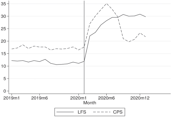
Source: LFS - Statistics Canada; IPUMSCPS (https://cps.ipums.org/cps/covid19.shtml, accessed June 10, 2021). Share of households in the month­ly CPS and LFS with no available information. The vertical line indicates February 2020. The LFS data includes all LFS households in the ten Canadian provinces.

One could argue that the rise in LFS non-response is due to a (drastic) change in the behaviour of potential respondents in response to the COVID-19 shock. It is more likely, however, that it has been caused by a shift in the conduct of Statistics Canada’s activities, as indicated by the timing of the increase—clearly concomitant to the start of the first national shutdown—and by its striking persistence. As of March 2020, federal agencies were instructed to adopt telework for the majority of their employees, i.e., federal workers were required to work from home whenever and wherever possible. Statistics Canada followed suit by suspending its field activities, and, as of January 2021, the LFS had yet to resume in-person interviews. This represented an important change in the data collection process: interviews could no longer be carried out in person, and as such, the LFS had to rely on its other two modes of collection (phone and online) for all interviews. For birth interview, the constraint was even more binding. It meant that the telephone was now the sole mode of interviewing, as online interviews are only carried out for subsequent interviews.

At first sight, one might think that the changes in collection methods were not dramatic (see Figure 2), since the vast majority of interviews were being conducted by phone or online prior to the pandemic (92.8 percent in 2019). However, a bit more context is required. The LFS has three modes of interview—in person, by phone, and online. In normal times, in-person interviews are conducted for a significant minority of birth interviews (34.5 percent in 2019).⁷ It is also the fall-back approach if phone interviewing is unsuccessful (e.g., the telephone number associated to the dwelling proved to be incorrect).⁸ These policies reflect the fact that the in-person mode of collection, although more expensive, is known to be effective for making first contact. As such, the halt of in-person interviews is expected to impact non-response rates. Due to the rotating nature of the sample, there is a potential for a significant stock-flow effect; the increased difficulties in making first contact in the incoming rotation can propagate to the ensuing months of the six-month window. A similar argument can be made for subsequent non-response given that in-person contact can help build a relationship with the household. It then follows that an apparently modest shift in interview modes can potentially generate a high and persistent increase in non-response rates, as seen in Figure 1.

Figure 2:

Proportions of Interviews by Mode of Collection (%)

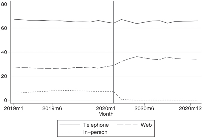
Source: LFS and authors’ calculations. Monthly cross-sectional samples of individuals aged 20 to 64, excluding full-time members of the armed forces and those living in the territories.

The suspension of in-person interviewing may only be part of the story, however. In pre-COVID times, telephone interviews were conducted from call centres. The adoption of telework arrangements at Statistics Canada required dispatching surveyors out of these centres, which could have resulted in efficiency losses. Given that it is a long-running survey, the LFS has experienced many expected and unexpected changes/shocks over the years, which can give us guidance on the impact of this most recent “reorganizational” effect. If past experiences are any indication, such changes do impact non-response rates due to the tight production deadline from enumeration to its public release. Having said this, the effects are of second order importance, and most importantly, temporary in nature as compared to what is observed in COVID-19 times. As an illustration, the Quebec non-response rate reached 11.4 percent during the January 1998 Quebec ice storm, only to come back to 6.2 percent (a more typical rate at that time) in the following month (Statistics Canada 1998). All in all, these facts point toward the idea that the suspension of in-person interviews is the main explanation behind the persistent surge in non-response rates.

Finally, it should be noted that the CPS also suspended in-person interviews as of March 2020, and that (as with the LFS) only a minority of interviews were carried out in person prior to the pandemic. However, contrary to the LFS, the CPS restarted in-person interviews in some areas of the country as of July 2020, expanding to the whole country beginning in September 2020. We take that CPS non-response rates did come back down after their initial surge around the restarting of field operations as further evidence, albeit indirect, of the importance of in-person interviews. Most importantly, the diverging patterns between two labour force surveys strongly suggest that one cannot simply assume that existing findings on how COVID-19 impacted American datasets automatically translates to Canadian ones.

Consequences of COVID-19 Non-Response for LFS Data

This section analyzes the consequences of the surge in non-response for LFS data. The empirical analysis of this section (and the remainder of the paper) relies on the confidential-use LFS files where we restrict our attention to civilian workers aged 20 to 64, and exclude those living in the territories. We impose the age restrictions so as to compare our findings with existing evidence regarding the COVID-19 shutdown.⁹

The Relative Importance of Birth vs. Subsequent Non-Response

At the core of our analysis is the distinction between birth and subsequent non-response. Subsequent non-response allows for the imputation of labour-market information to individuals using a “hot-deck” procedure that relies on their pre-existing information to find a donor.¹⁰ Obviously in the case of birth non-response, imputation is not possible, and the household remains out of the LFS sample as long as it cannot be reached by the surveyors. As such, the two types of non-response have different implications for labour-market estimates. Birth non-response could induce additional selection in the LFS sample along observable and non-observable characteristics that is correlated with labour-market outcomes. On the other hand, subsequent non-response resulting in imputation could introduce additional measurement or classification error.

We cannot directly attribute a share of non-response to one motive or another because we do not have information on the number of individuals living in-non-response households. However, we know from our restricted-use LFS files the number of individuals with fully imputed information, i.e., the number of individual whole record imputation (WRI) cases. This information allows us, with the help of some mild identifying assumptions, to disentangle the two types of non-response.

The solid line in Figure 3 tracks over time the sample that includes WRI cases—the unrestricted sample observed by researchers. The dashed line shows the sample size where WRI cases are excluded; it only accounts for individuals that were interviewed in the current month. Assuming that in the absence of COVID, the sample would have remained roughly similar beyond February 2020, i.e., around 70,000 as it has been for all of 2019, then the majority of non-response cases for June 2020 can be attributed to failed birth interviews: the decline of 10,000 in the dashed line represents birth non-response, whereas the 12,000 drop in the solid line represents both birth and subsequent non-response. A similar story holds true for other months. Figure 4 plots over time the size of the incoming rotation over time. It has certainly dropped due to COVID-19, especially between February and March, where it decreased by around 3,500 individuals. In the following months, the decline, albeit more tempered, still ranged from 2,000 to 3,000. Although substantive—given that the incoming sample stood at approximately 11,000 in February 2020—these drops can only account for a minor part of the total decline in response. This means that birth non-response is persistent: a subset of households have been harder to reach not just in their incoming month, but also in ensuing months.

Figure 3:

Sample Size with and without Whole Record Imputation (WRI)

Source: LFS and authors’ calculations. The solid line shows the total number of individuals in the full sample and the dash line shows the number of individuals after excluding those for whom LFS information has been fully imputed. The vertical line indicates February 2020. Monthly cross-sectional samples of individuals aged 20 to 64, excluding full-time members of the armed forces and those living in the territories.

Figure 4:

Sample Size of Incoming Rotations

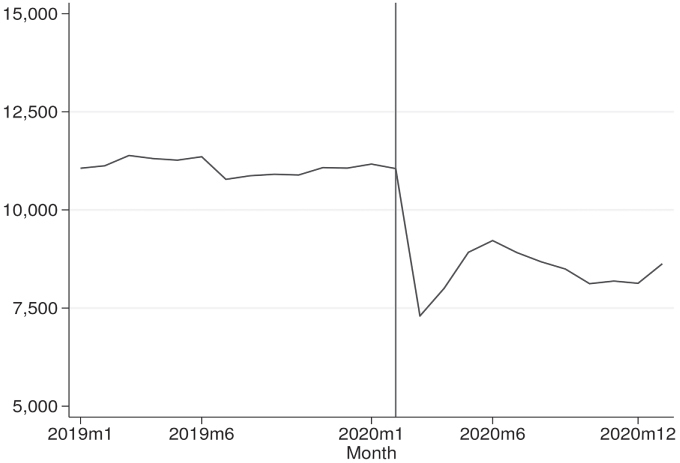
Source: LFS and authors’ calculations. Number of individuals in the incoming rotation group in each month of the LFS. The vertical line indicates February 2020. Monthly cross-sectional samples of individuals aged 20 to 64, excluding full-time members of the armed forces and those living in the territories.

If one imposes additional structure, i.e., assumes that the household non-response rates shown in Figure 1 also apply to individuals 20 to 64 year of age, one can quantify more precisely the importance of each type of non-response. Columns (2) and (3) of Table 1 show how birth and subsequent non-response have evolved over time, whereas columns (4) and (5), provide a further breakdown of birth non-response by whether it occurs in the first month, i.e., in the incoming rotation, or continues into the latter months of the six-month window. Table 1 clearly shows that prior to the pandemic, birth non-response was of secondary importance as compared to subsequent non-response. For example, in February 2020, birth and subsequent non-response were 3.8 percent and 8.1 percent, respectively. The striking feature is the rise in birth non-response in the COVID-19 era, reaching almost 24 percent in December 2020. The fact that birth non-response for the incoming rotation only grew by a few percentage points confirms our prior claim that first contact difficulties persist throughout the six-month window.¹¹

Table 1:

Non-Response Rates (%), by Type

		Response (1)	Birth Non-response (2)	Subsequent Non-response (3)	Birth Non-response
					Incoming (4)	Other (5)
2019	Jan	87.8	3.9	8.3	1.8	2.1
	Feb	88.0	4.0	8.0	1.7	2.3
	Mar	87.8	3.8	8.4	1.4	2.4
	Apr	88.4	3.5	8.1	1.4	2.1
	May	87.8	3.2	9.0	1.4	1.8
	Jun	88.2	2.9	8.9	1.3	1.6
	Jul	87.3	3.2	9.5	2.0	1.2
	Aug	88.9	2.7	8.4	1.8	0.9
	Sep	89.4	3.0	7.6	1.7	1.4
	Oct	89.3	2.8	7.9	1.6	1.2
	Nov	89.1	2.9	8.0	1.2	1.6
	Dec	88.4	3.2	8.4	1.2	2.0
2020	Jan	88.9	3.3	7.8	1.2	2.1
	Feb	88.1	3.8	8.1	1.5	2.3
	Mar	77.9	11.7	10.4	6.8	4.9
	Apr	76.5	13.5	10.0	5.6	7.9
	May	73.5	14.7	11.8	4.3	10.4
	Jun	71.8	16.4	11.8	3.8	12.6
	Jul	70.5	19.4	10.1	4.4	15.0
	Aug	70.5	20.5	9.0	4.8	15.7
	Sep	69.3	19.8	10.9	4.9	14.9
	Oct	70.0	21.9	8.1	5.6	16.3
	Nov	69.9	22.7	7.4	5.6	17.1
	Dec	69.2	23.9	6.9	5.7	18.3
2021	Jan	70.2	23.4	6.4	5.0	18.4

Notes: Monthly individual non-response rates (%) by type. Source: Statistics Canada and authors’ own calculations (see online appendix for details about the calculation of rates in columns (2) to (5)). Sample for individuals aged 20 to 64, excluding full-time members of the armed forces and those living in the territories. Columns (4) and (5) provides a breakdown of birth non-response: occurring in the first month of the six-month window, i.e., incoming rotation, (column (4)), or in an ensuing month (column (5)).

In-Person Interviews and Individual Characteristics

Given that in-person interviewing is relied upon when there are difficulties with the phone approach, one might expect selection into the LFS to become an issue when field operations were stopped. To investigate this possibility, we estimate the following linear probability model:

$$\mathrm{Pr}(inperso{n}_i=1|X_i)={\alpha }_0+X_i^{\text{'}}\alpha$$ (1)

where inpersoni is an indicator variable equal to one if individual i was interviewed in-person (and zero otherwise). Xi is a vector of socio-demographic characteristics comprising of binary variables for gender, age and education groups, and regions of residence.¹²

Table 2 shows regression results for March 2019 and July 2019 separately.¹³ The choice of 2019—the year prior to the pandemic—is to see whether the probability of being interviewed in “normal” times is correlated with socio-demographic characteristics. Two different months are chosen to account for possible seasonal patterns (as is observed in the non-response rate themselves). Since the analysis of the previous subsection indicates that high non-response rates are mostly accounted for by the falling number of birth interviews, we report regression results for this sub-population and for the incoming rotation (a further subset), in addition to that of the full sample. Finally, the regressions are unweighted as we are interested in estimating the share of in-person respondents within the sample itself (as opposed to what would be done in the case of estimating population moments).

Table 2:

Probability of Being Interviewed in Person, 2019, Unweighted

	March			July
	all (1)	birth only (2)	incoming only (3)	all (4)	birth only (5)	incoming only (6)
Female	−0.001 (0.002)	0.002 (0.008)	0.000 (0.008)	−0.003 (0.002)	−0.006 (0.009)	−0.012 (0.009)
20 to 29	0.014*** (0.003)	0.058*** (0.011)	0.056*** (0.012)	0.017*** (0.003)	0.063*** (0.012)	0.067*** (0.013)
50 to 64	−0.011*** (0.002)	−0.057*** (0.019)	−0.057*** (0.010)	−0.015*** (0.002)	−0.049*** (0.012)	−0.042*** (0.010)
Dropout	0.027*** (0.004)	0.049*** (0.015)	0.054*** (0.016)	0.031*** (0.004)	0.080*** (0.016)	0.075*** (0.017)
College	−0.005* (0.002)	−0.019* (0.010)	−0.020* (0.011)	−0.001 (0.003)	0.005 (0.011)	0.001 (0.012)
Bachelor +	−0.010*** (0.003)	−0.028** (0.011)	−0.025** (0.012)	−0.007*** (0.003)	−0.024** (0.012)	−0.033** (0.013)
East	0.037*** (0.003)	0.196*** (0.013)	0.209*** (0.013)	0.021*** (0.003)	0.110*** (0.014)	0.109*** (0.014)
Quebec	−0.012*** (0.003)	−0.020 (0.013)	−0.011 (0.013)	−0.021*** (0.003)	−0.093*** (0.013)	−0.119*** (0.014)
Prairies	0.041*** (0.003)	0.223*** (0.013)	0.232*** (0.013)	0.023*** (0.003)	0.101*** (0.013)	0.110*** (0.014)
Alberta	0.048*** (0.003)	0.297*** (0.014)	0.319*** (0.015)	0.013*** (0.004)	0.132*** (0.016)	0.132*** (0.017)
British Col.	0.038*** (0.003)	0.200*** (0.014)	0.215*** (0.015)	0.019*** (0.003)	0.086*** (0.014)	0.092*** (0.016)
Adj. R2	0.011	0.074	0.081	0.006	0.034	0.040
N	71,523	12,844	11,387	71,149	12,702	10,779

Notes: Probability of being interviewed in person conditional on individual characteristics. The full sample (i.e., all) covers individuals aged 20 to 64, excluding full-time members of the armed forces and those living in the territories. The samples in columns (2) and (5) are further restricted to only include individuals who are birth interviews. The samples in columns (3) and (6) are further restricted to only include individuals who are in the first month of the six-month window (i.e., incoming rotation). The dependent variable is an indicator for whether the household the individuals belong to was interviewed in person. Although not shown in the table, all regressions also include a constant. The reference group consists of males that are 30 to 49 years of age with no more than a high school degree who live in Ontario. All regressions are unweighted. Standard errors are shown in parentheses.

^*denotes statistical significance at 10%;

^**significance at 5%;

^***significance at 1%.

The findings of Table 2 indicate that the interview mode is non-random, especially for birth samples. The youngest and low-educated are more likely to be interviewed in person: in March 2019, i.e., just one year before the onset of COVID-19, individuals 20 to 29 years of age were 5.8 percentage point more likely to do an in-person interview than the 30 to 49-year olds. For dropouts, the likelihood was 4.9 percentage point higher than for individuals whose highest level of educational attainment was a high-school degree. In addition, the 50 to 64-year olds and those with a bachelor degree were less likely to be interviewed in person. The results are overall similar for July 2019; the most notable difference is the greater magnitude associated with the dropout coefficient for this month. There are also important disparities across provinces, with Albertans being the most likely to be interviewed in person (30 additional percentage points compared to Ontarians)—which would suggest distinctly different operating procedures across provinces.

When focusing on the incoming rotation, the results are essentially the same. This similarity is at least in part due to the important overlap between the two samples (all incoming interviews are by construction birth interviews), but this confirms that a non-randomly selected sub-sample of the households need to be reached in person very early on. Columns (1) and (4) of Table 2 assess how the interview modes are distributed across individuals in our full cross-section sample. The results are qualitatively the same (and still statistically significant), but much more subdued. Indeed, most of the in-person interviews are conducted in the incoming rotation, since this is in many cases used as a mean to establish initial contact. As such, the variation in interview modes across individuals is diluted when considering the full cross-section sample. Still, the differences across characteristics are significant even when one considers this sample.

How are these patterns linked with COVID-19 non-
response issues? That in-person interviewing is more likely to be used for low-educated and younger individuals suggests that they represent sub-populations that have been especially hard to reach during the pandemic. This might introduce biases in estimates based on incoming (and full) samples, since it has widely documented that these two groups have been—by far—among the hardest hit in terms of labour-market outcomes (Lemieux et al. 2020). Obviously, the remaining question is to what extent can LFS weights mitigate these issues, a question we will address shortly.

Birth Non-Response and Selection

Selection along Socio-Demographic Characteristics

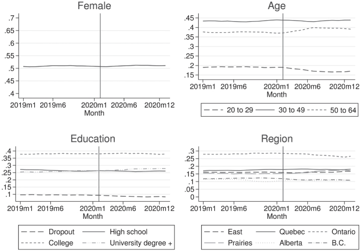
To further delve into potential selection issues, we explore how COVID-19 has impacted the socio-demographic structure of the LFS. Figure 5 presents unweighted sample shares by gender, age and education groups, and region of residence, for the incoming rotations over the January 2019–January 2021 period. Analyzing the structure of the incoming group is restrictive, but given the documented difficulties with first-contact interviews, it will provide a clear idea of how the sample of new entrants (to the survey) changed with the advent of COVID-19. The focus is on unweighted proportions as to examine the structure of the sample itself; when discussing the implications for labour-market estimates, we make use of weights.

Figure 5:

Proportions by Subgroups, Incoming Rotation, Unweighted

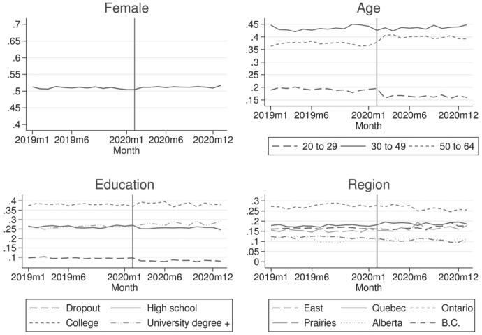
Source: LFS and authors’ calculations. The vertical line indicates February 2020. Monthly cross-sectional samples of individuals aged 20 to 64, excluding full-time members of the armed forces and those living in the territories.

Figure 5 shows a break in March 2021 along age and education lines. Rotations that started entering as of March 2021 are older and more educated than pre-COVID cohorts. The figure shows a clear drop in the proportion of individuals 20 to 29 years of age (around 20 percent in February vs. 16 percent in March), and a spike in the proportion of those aged 50 to 64 (36 percent vs. 40 percent). We see as well a decline in the proportions for the high-school and dropout groups, and an increase in the tertiary education groups (college and university). These findings are indicative of a significant and persistent impact of COVID-19 on response behaviours, consistent with the idea that the suspension of in-person activities created difficulties with initial contacts that have generated persistently high non-response rates. Moreover, the break in the trends of the age and education sample shares mirror well the documented facts of the previous section, which shows non-random assignment of interview modes along these two dimensions—with in-person interviews being more likely for the youngest, and the low-education individuals.

In Figure 6, we look at the same unweighted shares but for the full sample (i.e., all rotations), to assess how first contact difficulties propagate through the full sample. As one might have expected, one can observe a gradual change in sample structure starting in March 2021; given the rotating panel of the design, it takes a few months to get a critical mass of new entrants. This is especially visible along the age-group dimension: the 20 to 29 age-group share has been monotonically decreasing between March and June 2020, whereas the proportion of those 50 to 64 has been following the opposite trajectory. 50 to 64-year-olds account for 40 percent of the sample in June and onwards, vs. 36 percent in February (20 vs. 17 percent for youths). We observe a similar pattern along the education dimension, with a progressive increase in the share of highly-educated individuals in the sample.

Figure 6:

Proportions by Subgroups, All Rotations, Unweighted

Source: LFS and authors’ calculations. The vertical line indicates February 2020. Monthly cross-sectional samples of individuals aged 20 to 64, excluding full-time members of the armed forces and those living in the territories.

We complement the graphical investigation with a regression analysis. It allows us to carry out a series of statistical tests, and most importantly control for confounding factors. We do so by estimating the following linear probability model

$$\begin{array}{c}\mathrm{Pr}\left(d_{i,t}^m=1\mid X_{i,t},d_{i,t}^{2020}\right)\\ ={\beta }_o^m+X_{i,t}^{\prime }\beta +{\gamma }_0^m{d}_{i,t}^{2020}+\left(d_{i,t}^{2020}\times X_{i,t}^{\prime }\right){\gamma }^m,\end{array}$$ (2)

where $d_{i,t}^m$ is an indicator variable equal to one if individual i in year t is observed in calendar month m instead of February, i.e., the month just before the onset of the epidemic in Canada; X is the vector of socio-demographic variables as defined in equation (1); finally, d_i,t²⁰²⁰ an indicator variable taking the value one if the individual is observed in year t = 2020.

We estimate equation (2) for different sub-samples, i.e., using data for February and month m ∈ {March, May, July, September, November} in 2019 and 2020. Said differently, we first rely on February and March data for 2019 and 2020, and estimate the conditional probability of appearing in March. We then focus on the months of February and May to examine the probability of being observed in May, and so on. It should be noted that by incorporating 2019 data we can account for seasonal patterns in non-response. γm, the parameter vector of interest, measures how COVID-induced selection into non-response varies across observable characteristics. If the COVID-19 effect was truly random, then γ0m < 0 and γm = 0 for all m, with the negative intercept reflecting the increase in non-response observed in the COVID-era.

Table 3 shows the unweighted results for the incoming rotation. Consistent with the graphical analysis one still observes age and education profiles that persist over time—even when controlling for confounding factors. These effects tend to be economically and statistically significant. For instance, the probability 20 to 29-year olds appear in the March incoming rotation (instead of February) is 4.7 percentage points (p.p.) lower in 2020 than in 2019, relative to the 30 to 49-year-old group. Even more than six months after the initial shutdown, the youth age group has a 3.6 p.p. lower probability of appearing in the September incoming rotation. If one focuses on the education dimension, one sees that in COVID-19 times, individuals with a bachelor’s (or more) are 3.5 p.p. more likely to be a March entrant, and 3 p.p. more likely to be a September entrant (relative to the high-school individuals).

Table 3:

Probability of Being Observed in Select Months, 2019–2020, Incoming Rotation, Unweighted

	Mar (1)	May (2)	Jul (3)	Sep (4)	Nov (5)
Post COVID (γ0m)	−0.122*** (0.015)	−0.069*** (0.015)	−0.091*** (0.015)	−0.096*** (0.015)	−0.123*** (0.015)
Interaction terms with post COVID-19 indicator (γm):
Female	0.003 (0.010)	0.001 (0.010)	−0.000 (0.010)	−0.001 (0.010)	−0.000 (0.010)
20 to 29	−0.047*** (0.014)	−0.033** (0.014)	−0.044*** (0.014)	−0.036*** (0.014)	−0.021 (0.014)
50 to 64	0.013 (0.011)	0.006 (0.011)	0.016 (0.011)	0.002 (0.011)	0.002 (0.011)
Dropout	−0.035* (0.019)	−0.023 (0.019)	−0.020 (0.019)	−0.013 (0.019)	−0.019 (0.019)
College	0.033*** (0.013)	0.026** (0.012)	0.007 (0.013)	0.030** (0.013)	0.023* (0.013)
Bachelor +	0.035** (0.014)	0.027** (0.014)	0.028** (0.014)	0.010 (0.014)	0.020 (0.014)
East	−0.008 (0.016)	0.001 (0.015)	0.051*** (0.015)	0.038** (0.015)	0.068*** (0.015)
Quebec	0.028* (0.015)	0.021 (0.015)	0.053*** (0.015)	0.035** (0.015)	0.044*** 0.015)
Prairies	−0.020 (0.016)	0.019 (0.015)	0.076*** (0.015)	0.038** (0.016)	0.055*** (0.016)
Alberta	0.006 (0.017)	−0.022 (0.017)	0.051*** (0.018)	0.096*** (0.018)	0.018 (0.018)
British Columbia	−0.034** (0.017)	−0.042*** (0.017)	0.019 (0.017)	−0.000 (0.017)	−0.002 (0.017)
Adj. R2	0.013	0.005	0.006	0.006	0.009
N	40,865	42,369	41,873	41,583	41,446

Notes: Probability of being observed in select months, conditional on individual characteristics. Sample for individuals aged 20 to 64 in the incoming rotation, excluding full-time members of the armed forces and those living in the territories, and observed in February and a select month of 2019 and 2020. The select month is identified at the top of each column. The dependent variable is an indicator for whether the individual is observed in the select month. Although not shown in the table, all regressions also include the socio-demographic characteristics on their own and a constant. The reference group consists of males that are 30 to 49 years of age with no more than a high school degree who live in Ontario in February 2019. All regressions are unweighted. Standard errors are shown in parentheses.

^*denotes statistical significance at 10%;

^**significance at 5%;

^***significance at 1%.

To see how this incoming-rotation “entry” selection pattern affects the structure of the full LFS sample, we report in Table 4 unweighted regressions results for all rotations. Again, the estimates suggest a significant change in the structure of the sample along age and education dimensions. Consistent with the idea that non-response is primarily a birth issue, the changes in the sample structure come across gradually; there is no discernible effect for March, but when focusing on later months, the full LFS sample is clearly moving away from youths and low-educated individuals. As of November—eight months after the start of the epidemic—individuals 20 to 29 years of age are 2.8 p.p. less likely to be present in the sample than in the previous year (in comparison to the prime-age reference group); even more striking is the 4 p.p. lower probability of being part of the LFS sample for dropouts.

Table 4:

Probability of Being Observed in Select Months, 2019−2020, All Rotations, Unweighted

	Mar (1)	May (2)	Jul (3)	Sep (4)	Nov (5)
Post COVID (γ0m)	−0.019*** (0.006)	−0.035*** (0.006)	−0.054*** (0.006)	−0.059*** (0.006)	−0.064*** (0.006)
Interaction terms with post COVID-19 indicator (γm):
Female	−0.002 (0.004)	−0.002 (0.004)	−0.002 (0.004)	−0.002 (0.004)	−0.001 (0.004)
20 to 29	−0.006 (0.005)	−0.014** (0.005)	−0.028*** (0.005)	−0.032*** (0.005)	−0.028*** (0.005)
50 to 64	0.005 (0.004)	0.014*** (0.004)	0.021*** (0.004)	0.019*** (0.004)	0.021*** (0.004)
Dropout	−0.011 (0.007)	−0.019*** (0.007)	−0.033*** (0.007)	−0.035*** (0.007)	−0.040*** (0.007)
College	0.001 (0.005)	−0.003 (0.005)	−0.006 (0.005)	−0.006 (0.005)	−0.011** (0.005)
Bachelor +	0.004 (0.005)	0.004 (0.005)	0.006 (0.005)	0.004 (0.005)	−0.001 (0.005)
East	−0.002 (0.006)	0.001 (0.006)	0.018*** (0.006)	0.018*** (0.006)	0.027*** (0.006)
Quebec	0.003 (0.006)	0.007 (0.006)	0.015** (0.006)	0.016*** (0.006)	0.015** (0.006)
Prairies	0.001 (0.006)	0.011* (0.006)	0.034** (0.006)	0.051*** (0.006)	0.058*** (0.006)
Alberta	0.010 (0.007)	0.017** (0.007)	0.017** (0.007)	0.051*** (0.007)	0.070*** (0.007)
British Columbia	−0.009 (0.007)	−0.020*** (0.007)	−0.013** 0.007)	−0.007 (0.007)	−0.001 (0.007)
Adj. R2	0.000	0.001	0.003	0.003	0.004
N	278,100	274,042	270,784	269,746	267,969

Notes: Probability of being observed in select months, conditional on individual characteristics. Sample for individuals aged 20 to 64 in all rotations, excluding full-time members of the armed forces and those living in the territories, and observed in February and a select month of 2019 and 2020. The select month is identified at the top of each column. The dependent variable is an indicator for whether the individual is observed in the select month. Although not shown in the table, all regressions include the socio-demographic characteristics on their own and a constant. The reference group consists of males that are 30 to 49 years of age with no more than a high school degree who live in Ontario in February 2019. All regressions are unweighted. Standard errors are shown in parentheses.

^*denotes statistical significance at 10%;

^**significance at 5%;

^***significance at 1%.

We complement the analysis by observing the impact of COVID-19 on the structure of balanced panels. In the online appendix, we show the results for “new-entrant” mini panels (i.e., individuals are observed in the first two month of the six-month window) and the “full-rotation” panels (i.e., individuals are observed in any two consecutive months). To make our panel analysis comparable with the cross sectional one, the referenced month (i.e., February or month m) is taken to be the first period of the mini-panel. For example, the panel equivalent of being observed in March (as opposed to February), is the probability of being observed in the March–April panel (as opposed to the February–March panel).¹⁴

Unsurprisingly, the results for the new-entrant panel are similar to those of the incoming-rotation, and this for two related reasons. First, the new entrant mini-panel is, by construction, very similar to the incoming rotation; in both cases, the person must be part of the incoming rotation as of the referenced month. Second, the added panel restriction that the individual be also observed in the following month is not overly restrictive in COVID-19 times since we know that subsequent non-response is not the driving force behind the important rise in non-response. On the other hand, the results for “full-rotation” panels are more in line with those of the full cross-sectional sample. This holds true because in both cases the majority of individuals are not new to the sample.

Selection along Employment and Job Characteristics

We now analyze how employment and job characteristics correlate with non-response behaviours. A substantial literature has documented important heterogeneity in the impact of COVID-19 on labour-market outcomes across industries and occupations in Canada and elsewhere (see for e.g., Lemieux et al. 2020; Dingel and Neiman 2020; Baylis et al. 2022). It is therefore key to investigate whether workers who have been more exposed to the shock due to the characteristics of their job are more or less likely to be selected in the LFS sample in March 2020 onward.

Note that here, we cannot repeat the exercise of analyzing the change in the sample structure using pre-COVID and COVID-era data. Indeed, job characteristics have been directly impacted by COVID-19 beyond any change due to non-response; the COVID-led recession, for example, had a direct impact on the proportion individuals that are still employed and the type of job they hold. One possibility would be to look for evidence of selection based on the labour-market situation just before the epidemic—of those observed during the pandemic. However, since we are mainly interested in understanding birth non-response behaviours, this would require having retrospective information for new entrants in the LFS. Since such information is rather limited in the LFS, we cannot easily follow this approach.

We examine instead whether job characteristics that have been documented to be correlated with the intensity of COVID-19’s impact on individual outcomes are correlated with the mode of interview before COVID-19 (i.e., in 2019). In particular, we explore whether in-person respondents differ systematically from remotely-interviewed individuals, conditional on their job and socio-demographic characteristics. To do so, we estimate an augmented version of the linear probability model shown in equation (1), a version that includes job characteristics information as additional explanatory variables. The added variables consist of dummies for the employment status, quartile of the individual weekly salary, length of job tenure, and telework potential of the individual’s occupation.¹⁵ Considering individuals’ salary is motivated by studies that have documented a higher adverse impact of COVID-19 on low-earning workers (Lemieux et al. 2020) and accounting for job tenure is prompted by Brochu, Créchet, and Deng (2020) that suggest higher employment losses among low-tenure workers (controlling for age). Finally, the introduction of a telework variable follows the studies that have documented a more negative impact on individuals in occupation with low telework potential (e.g., for the US: Mongey, Pilossoph, and Weinberg 2021; for Canada: Baylis et al. 2022).¹⁶ It should be noted that we are interested in examining the presence of heterogeneity after controlling for characteristics that are taken into account in the design of the LFS weights. As such, we also introduce in the regression a set of dummies for the one-digit industry group of employed workers.

Table 5 shows striking differences along labour-market characteristics. In March 2019, low-salaried and low job-tenured workers, and those working in occupations with low potential for telework are more likely to be interviewed in person. Once again, the magnitude of these differences is higher for birth and incoming-rotation interviews than for the full sample (but the significance tends to be lower, probably due to due smaller sample size). For instance, in birth and incoming interviews, individuals in the second salary quartile are between 3 and 4 p.p. more likely to be interviewed in persons than those in the third quartile. Strikingly, in-person interviews are between 6 and 7 p.p. more likely for the employed with less than one year of tenure, than for the workers in more stable, long-lasting jobs (i.e., three years of tenure and more). Similar patterns are observed in July. Although we could not directly test for changes in the structure of the LFS sample along pre-COVID job characteristics, we interpret these results as indirect evidence that such changes have been occurring.

Table 5:

Probability of Being Interviewed in Person, Job Characteristics, 2019, Unweighted

	March			July
	all (1)	birth only (2)	incoming only (3)	all (4)	birth only (5)	incoming only (6)
Self-employed	−0.023*** (0.005)	−0.062*** (0.019)	−0.073*** (0.020)	−0.013*** (0.005)	−0.063*** (0.021)	−0.053** (0.023)
Employee	−0.027*** (0.004)	−0.070*** (0.018)	−0.073*** (0.019)	−0.021*** (0.005)	−0.061*** (0.020)	−0.050** (0.022)
Employee × earnings quartile 1	0.008** (0.004)	0.021 (0.015)	0.026 (0.016)	−0.001 (0.004)	−0.009 (0.016)	−0.012 (0.018)
Employee × earnings quartile 2	0.009*** (0.003)	0.031** (0.014)	0.036** (0.015)	0.003 (0.004)	−0.015 (0.015)	−0.012 (0.016)
Employee × earnings quartile 4	−0.002 (0.003)	−0.013 (0.015)	−0.003 (0.016)	−0.003 (0.004)	−0.044*** (0.016)	−0.048*** (0.017)
Employee × ten. 1–11 months	0.022*** (0.003)	0.067*** (0.014)	0.063*** (0.014)	0.023*** (0.003)	0.077*** (0.014)	0.074*** (0.015)
Employee × ten. 12–35 months	0.015*** (0.003)	0.051*** (0.012)	0.055*** (0.013)	0.007** (0.003)	0.029** (0.013)	0.015 (0.015)
Employee × telework	−0.008*** (0.003)	−0.021* (0.011)	−0.021* (0.011)	−0.008*** (0.003)	−0.014 (0.012)	−0.013 (0.013)
Socio-demographic controls	Yes	Yes	Yes	Yes	Yes	Yes
Employee × industry controls	Yes	Yes	Yes	Yes	Yes	Yes
Adj. R2	0.014	0.083	0.090	0.009	0.040	0.046
N	71,523	12,844	11,387	71,149	12,702	10,779

Notes: Probability of being interviewed in person conditional on individual and job characteristics. The full sample (i.e. columns (1) and (4)) covers individuals aged 20 to 64 in all rotations, excluding full-time members of the armed forces and those living in the territories. The samples in columns (2) and (5) are further restricted to only include individuals who are birth interviews. The samples in columns (3) and (6) are further restricted to only include individuals who are in the first month of the six-month window (i.e., incoming rotation). The dependent variable is an indicator for whether the household the individuals belong to was interviewed in-person. Although not shown in the table, all regressions include a constant. The reference group consists of non-employed males that are 30 to 49 years of age with no more than a high school degree who live in Ontario. All regressions are unweighted. Standard errors are shown in parentheses.

^*denotes statistical significance at 10%;

^**significance at 5%;

^***significance at 1%.

Non-Response and LFS Weights

This subsection examines the extent to which the LFS weights mitigate the potential selection biases linked to the COVID-induced surge in non-response. The LFS weighting methodology has a rich procedure. Key to our study is the “calibration” step, which is performed to ensure that (a) the weighted sample is representative of the entire population along key select dimensions including gender, age, and region of residence—but not education; and (b) it has a consistent structure across select labour-market dimensions over time (i.e., across ensuing months). For the latter, the weights are calibrated to ensure that individuals in the time t sample who also had been observed in t − 1, have similar t − 1 labour-market characteristics as those of the full t − 1 sample.¹⁷ The labour market dimensions that are accounted for include: (a) employment, unemployment, and participation (in aggregate and by sex/age groups); (b) employment by industry (corresponding roughly one-digit NAICS groups); (c) employment in the public and the private sector.¹⁸

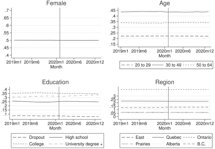
Since the weight calibration is performed to ensure that the sample is representative of the Canadian population across gender, age, and region, one should not, when weights are applied, be able to detect any changes as of March 2020 along these dimensions. Figures 7 and 8 display weighted sample shares by gender, age, region, and education, for the incoming rotation and the full sample, respectively. As expected, there is no apparent break in trends along the gender, age, and region dimensions (in direct contrast to what was observed for the unweighted shares shown in Figures 5 and 6). This result stands when controlling for confounding factors, i.e., when we run weighted regressions of equation (2) for the full cross-sectional sample (Table 6); the gender, age, and region effects that were clearly apparent in the unweighted regressions essentially vanish with the application of weights. Therefore, the weight adjustments have been mitigating the COVID-induced selection issues for some key socio-demographic characteristics.

Figure 7:

Proportions by Subgroups, Incoming Rotation, Weighted

Source: LFS and authors’ calculations. The vertical line indicates February 2020. Monthly cross-sectional samples of individuals aged 20 to 64, excluding full-time members of the armed forces and those living in the territories.

Figure 8:

Proportions by Subgroups, All Rotations, Weighted

Source: LFS and authors’ calculations. The vertical line indicates February 2020. Monthly cross-sectional samples of individuals aged 20 to 64, excluding full-time members of the armed forces and those living in the territories.

Table 6:

Probability of Being Observed in Select Months, 2019–2020, All Rotations, Weighted

	Mar (1)	May (2)	Jul (3)	Sep (4)	Nov (5)
Post COVID (γ0m)	0.004 (0.008)	0.005 (0.008)	0.008 (0.008)	0.008 (0.008)	0.006 (0.008)
Interaction terms with post COVID-19 indicator (γm):
Female	0.000 (0.005)	−0.000 (0.005)	−0.000 (0.005)	−0.000 (0.005)	−0.001 (0.005)
20 to 29	−0.001 (0.007)	−0.001 (0.007)	−0.001 (0.007)	−0.003 (0.007)	−0.002 (0.007)
50 to 64	−0.000 (0.006)	0.002 (0.006)	0.007 (0.006)	0.004 (0.006)	0.005 (0.006)
Dropout	−0.009 (0.010)	−0.019* (0.010)	−0.030*** (0.010)	−0.028*** (0.010)	−0.033*** (0.011)
College	−0.005 (0.007)	−0.011* (0.007)	−0.018*** (0.007)	−0.019*** (0.007)	−0.015** (0.007)
Bachelor +	−0.004 (0.007)	−0.004 (0.007)	−0.010 (0.007)	−0.009 (0.007)	−0.008 (0.007)
East	0.000 (0.007)	0.001 (0.007)	0.001 (0.007)	0.001 (0.007)	0.001 (0.007)
Quebec	0.001 (0.007)	0.002 (0.008)	0.003 (0.008)	0.003 (0.008)	0.003 (0.008)
Prairies	−0.000 (0.007)	0.000 (0.007)	0.000 (0.007)	0.000 (0.007)	0.000 (0.007)
Alberta	0.000 (0.008)	0.001 (0.008)	0.001 (0.009)	0.001 (0.009)	0.001 (0.009)
British Columbia	−0.000 (0.008)	−0.000 (0.008)	−0.000 (0.008)	−0.000 (0.009)	−0.000 (0.009)
Adj. R2	−0.000	−0.000	0.000	0.000	0.000
N	278,100	274,042	270,784	269,746	267,969

Notes: Probability of being observed in select months, conditional on individual characteristics. Sample for individuals aged 20 to 64 in all rotations, excluding full-time members of the armed forces and those living in the territories, and observed in February and a select month of 2019 and 2020. The select month is identified at the top of each column. The dependent variable is an indicator for whether the individual is observed in the select month. Although not shown in the table, all regressions also include the socio-demographic characteristics on their own and a constant. The reference group consists of males that are 30 to 49 years of age with no more than a high school degree who live in Ontario in 2019. All regressions are weighted. Standard errors are shown in parentheses.

^*denotes statistical significance at 10%;

^**significance at 5%;

^***significance at 1%.

It is worth noting that (along these same three dimensions) the weights also seem to considerably mitigate the selection issues for the panels (see online appendix). This might come as a bit of surprise since the weights are adjusted and calibrated based on estimates for the entire LFS sample. This holds true because non-response issue is mostly due to failed birth interviews (that persist through the six-month window), which means that the structure of the full-rotation panel samples is similar to that of the full cross-sectional sample (and the new entrant panel to that of the incoming rotation). We see this as good news for researchers that rely on the longitudinal dimension of the LFS.

However—by construction—the weights do not correct for other key dimensions, such as education, for which we have documented significant selection. In Table 6, the dropout coefficients are still highly significant and have magnitude close to these found for the unweighted regressions of Table 4.¹⁹ We should expect, therefore, that the weights have not been able to correct for the heterogeneity in job characteristics. Indeed, the previous section presents evidence suggesting heterogeneity in response behaviour conditional on socio-demographic and job characteristics.

Implications for COVID-19 Labour-Market Estimates

This section exploits the rotating-panel design of the LFS to examine the implications of selection for estimating the impact of COVID-19 on labour-market outcomes. Indeed, this rotating-panel design, combined with the fact that non-response is mainly associated with birth non-response (and, as such, with incoming rotations), provides variation in selection behaviours that is uncorrelated with labour-market outcomes.

Essentially, our approach consists of comparing the impact of COVID-19 on the individuals assigned to the rotations that entered the LFS before the onset of the epidemic in Canada (i.e., before March 2020), with those assigned to the rotations entering the LFS afterwards. Indeed, as we have argued so far, being assigned to a rotation that joined the LFS after the onset of COVID (which we call a post-COVID rotation) is associated with a lower likelihood of participating in the survey, presumably due to higher difficulties with reaching new entrants given the suspension of in-person interviews. On the other hand, we should expect the rotation assignment of individuals (for a given month) to be independent of their labour-market outcomes. As such, the differences between the two groups after the beginning of COVID-19 should reflect different selection patterns.

Hence, the key idea behind our proposed approach is that individuals assigned to pre-COVID rotations—the ones that entered the LFS prior to March 2020—have been exposed to a different selection rule than those assigned to post-COVID rotations. Before COVID-19, in-person interviews were available; however, this mode of interview was abruptly abandoned as of March 2020. As such, the post-COVID group have a higher non-response rate due to an exogenous factor—the assignment to a given LFS rotation.

Specifically, we propose the following model

$$E\left(y_{i,t}\mid d_{i,t}^r,d_{i,t}^{2020}\right)={\delta }_0+{\delta }_1{d}_{i,t}^r+{\delta }_2{d}_{i,t}^{2020}+{\delta }_3\left(d_{i,t}^r\times d_{i,t}^{2020}\right),$$ (3)

where yi,t is an individual labour-market outcome and dri,t is an indicator taking the value one if the individual is assigned to a rotation that entered the LFS in March or a later calendar month. Finally, d2020 is an indicator that equals one if the individual is observed in the year 2020. We estimate equation (3) for different sub-samples. We first estimate the model using March data for 2019 and 2020. We then repeat the exercise for each of the four subsequent months, separately. It should be noted that we only go up to July because this exercise requires having individuals that are part of rotations that entered the LFS prior to the pandemic. By July, only one rotation still meets this criterion.

The δ3 parameter measures the additional effect of COVID-19 that is associated with being assigned to a post-COVID rotation instead of a pre-COVID one. Given that the differences in labour-market outcomes across these two groups should reflect heterogeneity coming from their different selection rules, we interpret δ3 as reflecting differences due to selection induced by the COVID-19 disruption. Notice that the difference-in-difference design of our model allows us to control for seasonal effects that might generate differences across the rotations independently of COVID-19 (especially during the summer months, where non-response is usually high). In what follows, we consider the ensuing binary dependent variables: employment, employment-at-work, and non-participation. Considering employment-at-work is motivated by the dramatic decline in hours caused by COVID-19 in Canada (Lemieux et al. 2020), and by the historical increase in absences from work (Jones et al. 2020).

Before proceeding, we discuss the limitations of empirical approach by first focusing on the δ2 parameter. It measures the COVID-19 impact on individuals that have been assigned to an LFS sample prior to the pandemic. Yet, the group constituted by these individuals is clearly not exempted from selection, including selection caused by birth non-response. To illustrate this point, consider for example, two individuals (A and B) assigned to the rotation that entered the LFS in February 2020. Say individual A can be reached in February but not in March, whereas B cannot be reached in either month. Then as of March, individuals A and B are subsequent and birth non-respondents, respectively. Since δ2 measures the impact on a group where individuals like B are still present, it is still subject to a non-response bias (caused by birth non-response) that might have been reinforced by COVID-19. Therefore, our approach is not aimed at completely eliminating a potential non-response bias.

However, provided that (a) the bias is higher for individuals selected according to the post-COVID rule and that (b) it has the same sign across rotations, the δ3 coefficient indicates the direction of the bias.²⁰ Assumption (a) is justified by the results of the subsection discussing relative importance of birth vs subsequent non-response, indicating a clear increase in birth non-response driven by the rotations entering the LFS after the start of COVID-19. The reader might be more skeptical about assumption (b), but the results of the subsection concerning birth non-response and selection suggest that the selection patterns have essentially remained unchanged along key observable characteristics, across all rotations. At the very least, the estimated value of δ3 should be seen as a test of the null hypothesis that selection due to the suspension of in-person interviews is uncorrelated with the impact of COVID-19.

Table 7 shows OLS results for equation (3). Columns (1) to (5) report the findings where we impose dr =0, i.e., it estimates the unconditional impact of COVID-19 across all rotations, for March to July, whereas columns (6) to (10) report the results for the full regression, i.e., it allows the impact to vary across individuals assigned to pre- and post-COVID rotations. In the five months considered in panel A of Table 7, the point estimate of δ3 is always positive. This indicates that the surveyed individuals who have been assigned to a post-COVID rotation experienced lower (net) employment losses than individuals who have been assigned to prior rotations. For the two first months following the onset of COVID-19, the impact is strong—3.5 p.p. for March and 2.6 p.p. for April, as compared to the pre-COVID rotations—and significant at the 1 percent level. The magnitude and significance gradually diminish over the year, which is not surprising given that our treatment group is by construction less and less contaminated by birth non-response.

Table 7:

Pandemic Impact Across Pre- and post-COVID Entrants, 2019–2020, Weighted

	Mar (1)	Apr (2)	May (3)	Jun (4)	Jul (5)	Mar (6)	Apr (7)	May (8)	Jun (9)	Jul (10)
Panel A: Probability of employment
d2020	−0.031*** (0.003)	−0.110*** (0.003)	−0.102*** (0.003)	−0.066*** (0.003)	−0.047*** (0.003)	−0.037*** (0.003)	−0.119*** (0.004)	−0.109*** (0.005)	−0.074*** (0.005)	−0.056*** (0.008)
dr						−0.009 (0.006)	−0.003 (0.005)	−0.003 (0.004)	−0.007 (0.004)	−0.010* (0.006)
d2020×dr						0.035*** (0.010)	0.026*** (0.008)	0.015** (0.007)	0.012* (0.007)	0.011 (0.009)
N	136,975	134,322	132,917	131,860	129,659	136,975	134,322	132,917	131,860	129,659
Panel B: Probability of employment at work
d2020	−0.093*** (0.004)	−0.188*** (0.004)	−0.154*** (0.004)	−0.097*** (0.004)	−0.052*** (0.004)	−0.097*** (0.004)	−0.194*** (0.004)	−0.161*** (0.005)	−0.103*** (0.006)	−0.052*** (0.009)
dr						−0.012* (0.007)	−0.004 (0.005)	−0.004 (0.005)	−0.002 (0.005)	−0.005 (0.006)
d2020×dr						0.026** (0.011)	0.017** (0.008)	0.013* (0.007)	0.009 (0.007)	−0.000 (0.010)
N	136,975	134,322	132,917	131,860	129,659	136,975	134,322	132,917	131,860	129,659
Panel C: Probability of non-participation
d2020	0.016*** (0.003)	0.059*** (0.003)	0.042*** (0.003)	0.016*** (0.003)	0.007** (0.003)	0.020*** (0.003)	0.068*** (0.004)	0.051*** (0.004)	0.022*** (0.005)	0.014** (0.007)
dr						0.010* (0.006)	0.005 (0.004)	0.003 (0.004)	0.005 (0.004)	0.005 (0.005)
d2020×dr						−0.025*** (0.009)	−0.028*** (0.007)	−0.017*** (0.006)	−0.008 (0.006)	−0.009 (0.008)
N	136,975	134,322	132,917	131,860	129,659	136,975	134,322	132,917	131,860	129,659

Notes: estimates of the impact of COVID-19 on select labour-market outcomes. Sample for individuals aged 20 to 64 in all rotations, excluding full-time members of the armed forces and those living in the territories, and observed in a specific calendar month, in 2019 and 2020. The relevant month is identified at the top of each column. Columns (1) to (5) report estimates of the model (3) with the restriction δ₁ = δ₃ = 0 i.e., estimates for the unconditional impact across all rotations. Columns (6) to (10) report estimates for the full model (3) i.e., it allows the impact to vary across the individuals assigned to pre- and post-COVID incoming rotations. Although not shown in the table, all regressions include a constant. All regressions are weighted. Robust (Huber-White) standard errors are shown in parentheses.

^*denotes statistical significance at 10%;

^**significance at 5%;

^***significance at 1%.

The strong and gradually vanishing impact shown by Table 7 suggests the presence of an attenuation bias due to birth non-response when estimating the impact of COVID-19 on employment. As such, using the entire cross-section sample might understate the negative impact of the shock. This can be seen by comparing the coefficients of the restricted and unrestricted models (columns (1) to (5) and (6) to (10), respectively). For all the months considered, the estimated impact on the cross-sectional sample is less negative than for the group of pre-COVID LFS entrants only. This is in line with the analysis of our previous sections arguing that the individuals with the highest employment COVID-19 risk (in terms of observable characteristics) have been hardest to contact. The magnitude of these divergences is fortunately moderate. In March, the unconditional cross-sectional employment impact is −3.1 p.p., vs. −3.7 p.p. for the restricted sample; for the other months, the difference is at most equal to 1.1 p.p.

We find similar results for the impact of COVID-19 on the employment-at-work and non-participation probabilities: these probabilities have been less negatively affected for individuals in the March-onward rotations (panels B and C of Table 7). The pattern is similar to that of the employment estimates: the δ3 coefficient has a high magnitude and significance in March and April (less so for the employment-at-work probability than for participation, however), but the impact gradually vanishes. Again, the point estimates for the impact on the cross-section suggest a lower impact than for individuals assigned to a pre-COVID rotation, for all months. But, as for the employment estimates (Table 7), these differences remain moderate.

We now run placebo regressions using 2018−2019 data, for both employment and non-participation (see Table A.9 in the online Appendix). The employment and participation probabilities tend to be lower for the LFS entrants of March-2019 and after. There is, however, no significant rotation effect in March and April 2019, but for the late spring-early summer months the effect is substantial and significant. Here is a possible interpretation. Between 2018 and 2019, there have been aggregate employment gains. These gains have been presumably heterogeneous in the population, and one might expect that the most mobile groups have had the higher employment gains. Since mobility is relatively high in May–July, the most economically active individuals might have been harder to reach, especially those in incoming rotations. In sum, we might expect that when the economy is growing, birth non-response induces selection out of the LFS for the high-employment probability individuals, especially around the summer. The same reasoning can be made for participation, with the high-participation individuals being less represented in the incoming rotations of the spring and summer. Note that similar patterns hold when using earlier years for the placebo test (2015–2016, 2016–2017, and 2017–2018).

Consistent with this mobility-based interpretation are our results for OLS estimations for specific age groups (20 to 29 and 50 to 64-year olds). Conditional on belonging to these two groups, there is no rotation effect for 2018–2019. In other words, the effect seems to disappear when we condition on age. This suggests that the rotation difference for 2018–2019 can be explained by an age-related pattern, with youths becoming harder to reach in the spring-summer due to their higher mobility. Moreover, we find that for 2019–2020, the post-COVID rotation effect is very weak for this groups. An explanation is that there has been low heterogeneity in non-response behaviour within the youth group. The detailed results are shown in the online appendix.

However, for older workers, the picture depicting the COVID-19 labour-market impact is strikingly different as compared to youths. Table 8 shows the results for this age group, for 2019–2020. In March and April 2020, the employment effect of COVID-19 on 50-64-year-old workers assigned to incoming rotations of March and afterwards is much lower than for the pre-COVID LFS entrants. In March, the employment probability is 4.9 p.p. higher for the LFS entrants than for the incumbent, and 4 p.p. higher in April. The picture looks similar for participation. LFS entrants have been 3.1 p.p. less likely to not be in the labour force in March, and 3.3 p.p. in April. For this group, the point estimates of the coefficient of interest are much higher than for the entire population (Table 7). This suggests the presence of a potentially large bias due to selection for the 50–64-year-old individuals.

Table 8:

Pandemic Impact Across Pre- and Post-COVID Entrants, 2019–2020, 50–64 Years-Old, Weighted

	Mar (1)	Apr (2)	May (3)	Jun (4)	Jul (5)	Mar (6)	Apr (7)	May (8)	Jun (9)	Jul (10)
Panel A: Probability of employment
d2020	−0.018*** (0.006)	−0.077*** (0.006)	−0.064*** (0.006)	−0.043*** (0.006)	−0.031*** (0.006)	−0.026*** (0.006)	−0.091*** (0.007)	−0.068*** (0.008)	−0.037*** (0.010)	−0.054*** (0.014)
dr						−0.003 (0.011)	0.010 (0.008)	0.011 (0.008)	0.012 (0.008)	−0.006 (0.010)
d2020×dr						0.049*** (0.017)	0.040*** (0.013)	0.008 (0.012)	−0.009 (0.012)	0.028* (0.015)
N	51,307	50,694	50,425	50,631	50,209	51,307	50,694	50,425	50,631	50,209
Panel B: Probability of non-participation
d2020	0.012** (0.005)	0.039*** (0.006)	0.028*** (0.006)	0.013** (0.006)	0.006 (0.006)	0.018*** (0.006)	0.051*** (0.007)	0.035*** (0.008)	0.012 (0.009)	0.024* (0.013
dr						0.002 (0.010)	−0.009 (0.008)	−0.007 (0.007)	−0.005 (0.008)	0.005 (0.010)
d2020×dr						−0.031* (0.016)	−0.033*** (0.012)	−0.013 (0.011)	0.001 (0.012)	−0.022 (0.014)
N	51,307	50,694	50,425	50,631	50,209	51,307	50,694	50,425	50,631	50,209

Notes: estimates of the impact of COVID-19 on select labour-market outcomes. Sample for individuals aged 50 to 64 in all rotations, excluding full-time members of the armed forces and those living in the territories, and observed in a specific calendar month, in 2019 and 2020. The relevant month is identified at the top of each column. Columns (1) to (5) report estimates of the model (3) with the restriction δ₁ = δ₃ = 0 i.e., estimates for the unconditional impact across all rotation. Columns (6) to (10) report estimates for the full model (3) i.e., it allows the impact to vary across the individuals assigned to pre- and post-COVID incoming rotations. Although not shown in the table, all regressions include a constant. All regressions are weighted. Robust (Huber-White) standard errors are shown in parentheses.

^*denotes statistical significance at 10%;

^**significance at 5%;

^***significance at 1%.

Discussion

This paper first documents the significant and persistent rise in household non-response rates in the Canadian Labour Force Survey during COVID-19. Non-response rates have reached and stabilized at an unprecedented level of 30 percent, up from the 10–12 percent range observed in the decade prior to the pre-COVID era. Most of this surge can be plausibly attributed to the interruption of in-person interviews at Statistics Canada. The increase in non-response has not been random: those who were vulnerable to the COVID-19 economic shock (such as youths, low educated, workers in low-earning/low-tenure jobs with limited potential for telework) have been harder to reach. Furthermore, the LFS weights do not fully mitigate selection, particularly along key dimensions such as education, the length of job tenure, and individuals’ occupation. Consistent with these LFS selection patterns, we provide evidence that existing estimates have underestimated the impact of the pandemic on aggregate employment and participation, especially during the first wave in March and April 2020.

There are, however, reasons for optimism. Our results do not change the commonly accepted narrative for the trajectory of aggregate labour-market activity in COVID-19 times—that of tremendous but short-lived decline at the onset of the epidemic, followed by a sharp, vigorous rebound after the easing of the first-wave lockdown. Indeed, the biases we document do not contradict the qualitative features nor the order of magnitude of existing estimates of the changes in employment and participation. In addition, we do not find evidence of significant biases beyond the first wave, when the economy initiated its recovery. Furthermore, when put into perspective with other surveys in Canada and elsewhere, the size of the disruption on LFS data can be considered relatively modest given the high severity of the COVID-19 shock. It is clear that an LFS non-response rate of 30 percent more than rivals most existing surveys, even before COVID-19.

Another reason for optimism that has practical implications for research is that the rise in subsequent non-response has been moderate, which means that panel attrition has not significantly worsened. This is reflected in our results that the structure of the panels (in terms of socio-demographic characteristics) has remained similar to that of cross-section samples, and that key aggregate labour-market statistics differ modestly across cross-section and panel samples during COVID-19 (Brochu et al. 2020). Researchers interested in conducting longitudinal analysis should therefore feel reassured that panels are not contaminated by selection issues more severe than in the cross-section.

The optimistic interpretation comes with the following caveats. First, our empirical exercise is inconclusive about the size of COVID-19 biases as it only indicates signs and lower bounds. The true bias could be much higher than suggested by our results depending on how difficult it was for surveyors to reach the rotations that entered the survey just prior to the pandemic. Second, the analysis focuses on birth non-response issues rather than subsequent non-response, as the rise in the latter is of second order importance. Yet, the temporary rise in subsequent non-response rates should nonetheless be of concern: over the March to September 2020 period, the labour market information of one out of eight individuals was fully imputed, as opposed to one out of twelve in the pre-COVID period. The use of whole record imputation may make the resulting dataset appear to evolve in a consistent way over time while not necessarily reflecting how these aspects of the economy did in fact evolve. Third, our analysis focuses on aggregate estimates. Since selection is non-uniform across individuals, our conclusions for the aggregate levels do not immediately apply to subgroups as suggested by our results for individuals of age 50–64. Researchers interested in subgroup outcomes (e.g., immigrants, single parents) should exert care when gauging the robustness of their results using COVID-time data, particularly at the onset of the pandemic.

We suggest the following: researchers with access to the LFS Master files should take advantage of information regarding individuals’ rotation assignments to examine the robustness of their results across samples of pre- and post-COVID entrants. Moreover, those interested in examining the early stages of the COVID-19 period using longitudinal analysis may want to construct their two-month mini panels using all rotations (i.e., any two consecutive months) instead of just the first two months of the six-month window, as the latter is more likely to be contaminated by selection. Of note, the information on individuals’ rotations is not made available in the public-use files. Our analysis suggests that providing such information to researchers who rely on public-use data would be beneficial for producing robust analyses for years to come.

It would be highly informative to reassess the economic impact of COVID-19 when relevant administrative datasets become available to researchers. As of January 2022, all LFS interviews are still conducted remotely; the shift in data collection we document has persisted so far. This makes it crucial to evaluate the impact of the suspension of face-to-face interviews on the quality of LFS data. It is our belief that only with the eventual resumption of field operations (with the opportunity of carrying out in-person interviews), can the non-response rate return to levels that we have been accustomed to seeing from this flagship survey.

References

- Achou, B., Boisclair D., d’Astous P., Fonseca R., Glenzer F., and Michaud P.-C.. 2020. “Early Impact of the COVID-19 Pandemic on Household Finances in Quebec.” Canadian Public Policy 46(S3):S217–35. 10.3138/cpp.2020-087 [DOI] [PMC free article] [PubMed] [Google Scholar]
- Baylis, P., Beauregard P.-L., Connolly M., Fortin N.M., Green D.A., Gutiérrez-Cubillos P., Gyetvay S., Haeck C., Molnár T.L., Simard-Duplain G., Siu H.E., teNyenhuis M., and Warman C.. 2022. “The Distribution of COVID-19-Related Risks.” Canadian Journal of Economics 55(S1):172–213. 10.1111/caje.12540. Medline:34898684 [DOI] [PMC free article] [PubMed] [Google Scholar]
- Beland, L.-P., Brodeur A., Mikola D., and Wright T.. 2022. “The Short-Term Economic Consequences of COVID-19: Occupation Tasks and Mental Health in Canada.” Canadian Journal of Economics 55(S1):214–47. 10.1111/caje.12543 [DOI] [PMC free article] [PubMed] [Google Scholar]
- Beland, L.-P., Fakorede O., and Mikola D.. 2020. “Short-Term Effect of COVID-19 on Self-Employed Workers in Canada.” Canadian Public Policy 46(S1):S66–81. 10.3138/cpp.2020-076 [DOI] [PMC free article] [PubMed] [Google Scholar]
- Blit, J. 2020. “Automation and Reallocation: Will COVID-19 Usher in the Future of Work?” Canadian Public Policy 46(S2):S192–202. 10.3138/cpp.2020-065 [DOI] [PMC free article] [PubMed] [Google Scholar]
- Brochu, P. 2021. “A Researcher’s Guide to the Labour Force Survey: Its Evolution, and the Choice of Public Use Versus Master Files.” Canadian Public Policy 47(3):335–57. 10.3138/cpp.2020-046 [DOI] [Google Scholar]
- Brochu, P., Créchet J., and Deng Z.. 2020. “Labour Market Flows and Worker Trajectories in Canada During COVID-19.” CLEF Working Papers Series No. 32. At https://clef.uwaterloo.ca/wp-content/uploads/2020/10/CLEF-032-2020-Brochu-et-al.pdf.
- Brochu, P., and Green D.A.. 2013. “The Impact of Minimum Wages on Labour Market Transitions.” Economic Journal 123(573):1203–35. 10.1111/ecoj.12032 [DOI] [Google Scholar]
- Bryan, K.A., Buajitti E., Rosella L.C., and Goel V.. 2021. “The Economic and Long-Term Health Consequences of Canadian COVID-19 Lockdowns.” Canadian Public Policy 47(2):281–300. 10.3138/cpp.2020-134 [DOI] [PMC free article] [PubMed] [Google Scholar]
- Deng, Z., Morissette R., and Messacar D.. 2020. “Running the Economy Remotely: Potential for Working from Home During and after COVID-19.” StatCan COVID-19: Data to Insights for a Better Canada, no. 26. Statistics Canada Cat. no. 45280001, Ottawa. At https://www150.statcan.gc.ca/n1/en/pub/45-28-0001/2020001/article/00026-eng.pdf?st=pK3fu_Fc. [Google Scholar]
- Dingel, J.I., and Neiman B.. 2020. “How Many Jobs Can Be Done at Home?” Journal of Public Economics 189(C). 10.1016/j.jpubeco.2020.104235. Medline:32834177 [DOI] [PMC free article] [PubMed] [Google Scholar]
- Forsythe, E., Kahn L.B., Lange F., and Wiczer D.. 2020. “Labor Demand in the Time of COVID-19: Evidence from Vacancy Postings and UI Claims.” Journal of Public Economics 189(C). 10.1016/j.jpubeco.2020.104238. Medline:32834178 [DOI] [PMC free article] [PubMed] [Google Scholar]
- Gallacher, G., and Hossain I.. 2020. “Remote Work and Employment Dynamics under COVID-19: Evidence from Canada.” Canadian Public Policy 46(S1):S44–54. 10.3138/cpp.2020-026 [DOI] [PMC free article] [PubMed] [Google Scholar]
- Jones, S.R.G., Lange F., Riddell W.C., and Warman C.. 2020. “Waiting for Recovery: The Canadian Labour Market in June 2020.” Canadian Public Policy 46(S2):S102–18. 10.3138/cpp.2020-078 [DOI] [PMC free article] [PubMed] [Google Scholar]
- Jones, S.R.G., Lange F., Riddell W.C., and Warman C.. 2021. “Canadian Labour Market Dynamics during COVID-19.” CLEF Working Papers Series No. 37.
- Jones, S.R.G., and Riddell W.C.. 2019. “Unemployment, Marginal Attachment, and Labor Force Participation in Canada and the United States.” Journal of Labor Economics 37(S2):S399–441. 10.1086/703399 [DOI] [Google Scholar]
- Koebel, K., and Pohler D.. 2020. “Labor Markets in Crisis: The Causal Impact of Canada’s COVID-19 Economic Shutdown on Hours Worked for Workers across the Earnings Distribution.” CLEF Working Papers Series No. 25.
- Lemieux, T., Milligan K., Schirle T., and Skuterud M.. 2020. “Initial Impacts of the COVID-19 Pandemic on the Canadian Labour Market.” Canadian Public Policy 46(S1):S55–65. 10.3138/cpp.2020-049 [DOI] [PMC free article] [PubMed] [Google Scholar]
- Lundy, M. 2021. “‘Your Flying Blind’: In Nunavut, a Data Crisis Is Brewing.” Globe and Mail, Online edition, 6 October. Accessed 4 March at https://www.theglobeandmail.com/business/article-youre-flying-blind-in-nunavut-a-data-crisis-is-brewing/.
- Messacar, D., Handler T., and Frenette M.. 2021. “Predicted Earnings Losses from Graduating during COVID-19.” Canadian Public Policy 47(2):301–15. 10.3138/cpp.2020-109 [DOI] [PMC free article] [PubMed] [Google Scholar]
- Mongey, S., Pilossoph L., and Weinberg A.. 2021. “Which Workers Bear the Burden of Social Distancing?” Journal of Economic Inequality 19(3):509–26. 10.1007/s10888-021-09487-6. Medline:34366750 [DOI] [PMC free article] [PubMed] [Google Scholar]
- Montenovo, L., Jiang X., Lozano-Rojas F., Schmutte I., Simon K., Weinberg B.A., and Wing C.. 2022. “Determinants of Disparities in COVID-19 Job Losses.” Demography 59(3):827–55. 10.215/00703370-9961471 [DOI] [PMC free article] [PubMed] [Google Scholar]
- Qian, Y., and Fuller S.. 2020. “COVID-19 and the Gender Employment Gap among Parents of Young Children.” Canadian Public Policy 46(S2):S89–101. 10.3138/cpp.2020-077 [DOI] [PMC free article] [PubMed] [Google Scholar]
- Rivera Drew, J.A., Flood S., and Warren J.R.. 2014. “Making Full Use of the Longitudinal Design of the Current Population Survey: Methods for Linking Records across 16 Months.” Journal of Economic and Social Measurement 39(3):121–44. 10.3233/jem-140388. Medline:26113770 [DOI] [PMC free article] [PubMed] [Google Scholar]
- Rothbaum, J., and Bee A.. 2021. “Coronavirus Infects Surveys, Too: Nonresponse Bias and the Coronavirus Pandemic in the CPS ASEC.” SEHSD Working Paper Number 2020–10.
- Sheridan, M., Drew D., and Allard B.. 1997. “Response Rate and the Canadian Labour Force Survey: Luck or Good Planning.” Proceedings of Statistics Canada Symposium 96, Nonsampling Errors. Ottawa:67–75. [Google Scholar]
- Statistics Canada . 1998. Labour Force Survey: Quality Report Surveys, 0198 to 0698, Statistics Canada Cat. no. 71-0004, Ottawa. [Google Scholar]
- Statistics Canada . 2017. Methodology of the Canadian Labour Force Survey, Statistics Canada, Cat. no. 71-526-X, December, Ottawa. [Google Scholar]
- US Bureau of Labor Statistics . 2020. “The Impact of the Coronavirus (COVID-19) Pandemic on the Employment Situation for July 2020.” At https://www.bls.gov/COVID19/employment-situation-COVID19-faq-july-2020.htm.
Associated Data
This section collects any data citations, data availability statements, or supplementary materials included in this article.