Sequence Coverage Visualizer: A web application for protein sequence coverage 3D visualization

Abstract

Protein structure defines protein function and plays an extremely important role in protein characterization. Recently, two groups of researchers from DeepMind and Baker lab have independently published protein structure prediction tools that can help us obtain predicted protein structures for the whole human proteome. This enabled us to visualize the entire human proteome using predicted 3D structures for the first time. To help other researchers best utilize these protein structure predictions in proteomics experiment, we present the Sequence Coverage Visualizer (SCV), http://scv.lab.gy, a web application for protein sequence coverage 3D visualization. Here we showed a few possible usages of the SCV, including the labeling of post-translational modifications and isotope labeling experiments. These results highlight the usefulness of such 3D visualization for proteomics experiments and how SCV can turn a regular proteomics experiment (identified peptide list) into structural insights. Furthermore, when used together with limited proteolysis, we demonstrated that SCV can help to compare different protein structures from different sources, including predicted ones and existing PDB entries. We hope our tool can provide help in the process of improving protein structure prediction accuracy. Overall, SCV is a convenient and powerful tool for visualizing proteomics results in 3D.

Graphical Abstract

Introduction

To date, most of the proteomics experiments are conducted using the bottom-up proteomics method. Proteins are digested by sequence grade trypsin into smaller peptides and then separated and identified by LC-MS/MS. Comparing to other proteomics methods, bottom-up proteomics is by far the most efficient way to identify and quantify thousands of proteins within hours. However, since the analyte is not the whole protein but rather digested tryptic peptides, bioinformatics is needed to assemble all the available information to infer the original proteins. This entire process makes the protein sequence coverage, i.e., the ratio of total observed protein sequence length to total protein length, an essential parameter for bottom-up proteomics. The typical average protein sequence coverage of a conventional bottom-up proteomics experiment varies from less than 10% to over 90%, depending on the complexity of the sample and the sample processing methods. The sequence coverage percentage generally increases monotonically as the digestion is more and more complete through time.¹

Noting this phenomenon, limited proteolysis methods have been developed to use various digestion time points to differentiate the easy-to-digest and hard-to-digest parts of the proteins^2-4. It is reasonable to believe that the initial digested peptides are from the more accessible regions of the protein, and the later digested peptides are generally from hard-to-access regions. When a time series is created using limited proteolysis, we can easily map all the identified peptides from different time points to the protein sequence. Even better, if we could map all these peptides onto a 3D model of the protein, we could see the sequence coverage in 3D and validate if the identified peptides are from the same region or not. When the sequence coverage increases over time, we can further visualize it in space to see how protease digests the protein over time. Such visualization will significantly improve our understanding of the protease digestion process and even help us to refine protein structures further. However, this was not entirely possible in the past, as crystallography, NMR, and Cryo-EM protein structures cover only a limited portion of the known proteome. Recently, two groups of researchers, one from DeepMind and one from the Baker lab, independently published two powerful tools for protein structure prediction^5-7. Although there are still debates on the validity of the predicted structures, it is no doubt that these algorithms represent the best prediction methods we can have to date. More importantly, these tools and the published data make it possible to visualize the majority of human proteins for the first time.

Using these predictions, we created Sequence Coverage 3D Visualizer (SCV), http://scv.lab.gy as a free web application with easy-to-use interface and a programmatically accessible application programming interface (API). As a web application, SCV supports most of the modern web browsers and multiple platforms (Windows, Linux, MacOS, Android, iOS, etc.) and can be used on mobile devices. In addition to the web application, SCV can also be used locally to generate 3D models of protein sequence coverage using Python scripts, similar to previously published tools such as AlphaMap and StructureMap ^8,9. SCV can assist researchers worldwide to easily visualize proteomics results in 3D, and further explore the structural aspect of their data. To show the potential usage and usefulness of SCV, here we demonstrate multiple examples to highlight the features of SCV. These examples are provided here to demonstrate the functionality and potential usages of SCV. Using previously published isotope labeling data, we showed that SCV can be used to visualize and compare the positions of differentially labeled amino acid residues. When used together with limited proteolysis data of native proteins, SCV could visualize the digestion progress and therefore compare predicted structures to existing PDB entries. Such comparison may serve as an important step towards the validation of predicted structures from both AlphaFold2 ⁵ and RoseTTAFold ⁷. Overall, we demonstrated that SCV can be easily used to convert proteomics results into 3D structural insights.

Results and Discussion

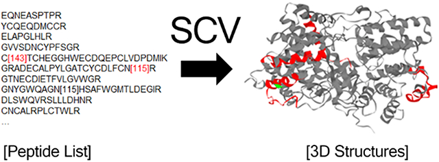
The Sequence Coverage 3D Visualizer (SCV) can be accessed at http://scv.lab.gy/. The basic function of SCV is to visualize protein sequence coverage in 3D using the peptide list identified from experiments (Fig. 1). SCV has a user-friendly web interface (Fig. 1) which allows the user to directly copy and paste an experimentally identified peptide list. When post-translational modifications (PTMs) are included in the results as numbers in brackets (“[]”), they will be automatically detected and visualized with different colors. User can also use curly brackets together with brackets “{}[group_name]” to highlight a group of peptides on the model. The background color and the color of each PTM can be customized easily through the interface. User can select the species (currently supports human, mouse and rat data), and then all the peptides are mapped to the corresponding UniProt reference database. Peptides are mapped directly to the protein sequence, without prior knowledge of the protease specificity. This allows the user to use peptides identified from different proteases to be mapped on the same protein model. All detected proteins will be listed with gene name, UniProt identifier and a brief description of the protein. In addition, a linear sequence coverage map is generated for each protein entry to show the positions of detected peptides. When selected from the protein list, a rotating 3D structure is generated, with red color highlighting the covered sequence and other user-selected colors to highlight the PTMs. User can interactively highlight any of the region by selecting it from the 2D sequence map. By default, SCV uses AlphaFold’s predicted 3D models of the proteins as it covers the majority of human proteome and provide good accuracy for most known proteins we tested. Custom 3D model mapping is supported through PDB file upload. When users upload a PDB file of a protein or protein complexes, the uploaded structure will be used for visualization instead of the default predicted structure. To facilitate the integration of SCV into other tools, we also provide a programmatically API, which is explained in detail together with the offline source codes of the SCV at https://github.com/Gaolaboratory/SCV.

Figure 1.

Overview of SCV web application input and output. SCV uses peptide list and species information to generate a list of proteins with linear sequence coverage and let users select the protein to visualize in 3D. By default, AlphaFold-predicted structures are used; users can also upload 3D structure in PDB format to customize 3D models. Post-translational modifications noted in brackets are automatically detected and can also be visualized by custom colors.

Once submitted by user, the peptide list is processed by our backend Node.js server and custom Python scripts running on our server. A typical response of a few thousand peptides and a few hundred proteins takes only seconds to process. A permanent link is provided to reference the result and it can be shared with others and inspected later. The protein list is sorted by sequence coverage percentage, from high to low. The 3D visualization is rendered using GLmol¹⁰, a WebGL library, and Three.js¹¹, a JavaScript library for 3D graph display. Our interactive 3D visualization allows the user to move and rotate the protein to make close observations easily. SCV works on all major web browsers on both desktop and mobile devices. SCV is open-source and freely available under Creative Commons license (CC BY-NC-SA 3.0) for any non-commercial use.

Isotope labeling visualization

SCV could be used to visualize and validate isotope-labeled proteomics results by inspecting the spatial relationship between differentially labeled residues. Here, we used the covalent protein painting data from Bamberger et al.¹² to demonstrate its usage. In this paper, Bamberger et al. described a method to differentially label “heavy” and “light” dimethyl groups to proteins before and after protein unfolding. In native form, proteins are first labeled in vivo with “light” dimethyl groups through reductive amination. The surface or more exposed lysine groups of the protein are therefore labeled. Later, with denaturing conditions, unfolded proteins are labeled again with “heavy” dimethyl groups. Because the more accessible lysine groups have already been labeled in the previous step, only the newly exposed lysine groups are labeled with the “heavy” dimethyl groups, making it possible to differentiate lysine groups with different accessibility. Here, we picked one of the proteins from the experiment, the GAPDH, as an example to show how SCV could be used to visualize different isotopes of the “heavy” and “light” dimethyl groups on lysine (Fig. 2). As shown in Fig. 2a, the whole GAPDH protein is visualized in 3D and the detected sequences are covered in red color. The green residues are the lysine groups labeled with the “light” label and the blue residues are the lysine groups labeled in “heavy”. We have included 4 different views (Fig. 2b, front, top, left, right) from the SCV, the actual 3D visualization is more insightful than these 2D views. This visualization result shows that mild heat shock will increase the accessibility of the lysine groups, as described in the paper. The interactive interface of SCV that allows free rotation and zoom in/out enabled us to inspect the result in space and better understand the spatial relationship between the native and unfolded forms of the protein. With the help of SCV, 3D visualization of both “heavy” and “light” labeling of all the protein described in this paper can be generated within seconds without any expert knowledge or the use of additional tools.

Figure 2.

Isotope labeling visualization of GAPDH protein labeled with both heavy and light dimethyl. a) 3D visualization generated by SCV. Red: covered sequence; grey: not covered sequence; green: light isotope label; blue: heavy isotope label. b) transparency adjusted model to highlight the position of the labeled residues at different angles.

3D visualization of digestion through time

Limited proteolysis has been used to obtain protein structural information in previous research.^2,12 When a protein is only allowed to be digested by a protease for a limited time, easy-to-digest regions are detected in early time points while hard-to-digest regions are detected later. When plotted through time, the appearance of different peptides from different regions of the protein can be correlated to the accessibility of the region (Fig. 3). When proteins are digested in their native form, limited proteolysis can be used to determine the more accessible surfaces, which are often digested first, followed by the less accessible regions, till complete unfolding. Here, we performed native digestion of HEK293 cell lysate using trypsin at four different time points: 1, 2, 4, 20 hours. At each time point, digested peptides are removed from the system by a 3.5k MWCO dialysis membrane. The digested peptides at each time point are separated and identified by LC-MS/MS. All the data of our limited-proteolysis is deposited at PRIDE (dataset PXD032786)

Figure 3.

Limited proteolysis of native proteins visualized by SCV. Glutathione S-Transferase Pi 1 (GSTP1), Profilin 2 (PFN2), Phosphoglycerate Kinase 1 (PGK1) are selected as examples here. Red color highlights the detected peptides at each of the four time points, grey color shows the undetected portion of the protein.

When we combine the data from all four time points, and visualize them by SCV, we can easily see the progression of the digestion of trypsin (Fig. 3). In the three examples shown in Fig. 3, proteins are gradually digested over time. In the case of GSTP1, the outer regions are first observed as early as 2-hour. More inner regions of the GSTP1 are then followed in 4-hour and 20-hour time points. PFN2, on the other hand, is digested first at one of the helix regions at the surface, then followed by beta-sheet region inside. At the final 20-hour time point, the innermost beta-sheet region of PFN2 is eventually observed. In the case of PGK1, some outer regions are digested only in late time points, showing a possible resistance to digestion or possibly an early unfolding. The early unfolding might be a result of the digestion of key connection regions at an early time point. We need to point out that the undetected regions (grey) are mostly not due to resistance to digestion, but rather caused by low detectability of the corresponding peptides by mass spectrometry, either due to low ionization or non-ideal cleavage site arrangement. This visualization (Fig. 3) clearly shows the power of SCV to assist the structural investigation by proteomics experiments.

Compare predicted structures

The predicted protein structures by AlphaFold2 and RoseTTAFold are proven to be among the most accurate prediction algorithms published to date. However, many challenging structures cannot be accurately predicted, e.g., intrinsically disordered proteins. Existing prediction models are trained by the currently available 3D structures from X-ray crystallography, NMR, and Cryo-EM experiments and therefore perform very well on known structures and domains as they are included in the training set. These predictions may also provide satisfactory results for many proteins with unknown structures but mainly composed of domains similar to known structures. However, there is no easy way to directly validate the accuracy of the predicted results for the unknown proteins composed mainly with unknown domains, as these unknown domains have never been characterized by an experiment.

On the other hand, all predicted structures must follow the same physical rules as the other known proteins. The accessibility of each region, defined by the predicted structure, must be consistent with the experimental observation. This gives us a unique opportunity to use our limited proteolysis results to validate and compare different prediction results. Here, we used data from our limited proteolysis experiments and mapped all observed peptides onto the structure predicted by AlphaFold2 and RoseTTAFold. Here we are showing three examples, the phosphohydroxythreonine aminotransferase 1 (PSAT1), Ribosomal Protein L18a (RPL18A) and Far Upstream Element Binding Protein 1 (FUBP1). The peptide mappings at 1, 2, 4 and 20 hours on both AlphaFold predicted structures and RoseTTAFold predicted structures are shown in Supp. Fig. 1-3. The predicted structures of PSAT1 and RPL18A from both algorithms are very similar with only minor differences. In contrary, the predicted structures of FUBP1 are very different by the two algorithms (Supp. Fig. 3). With our time-series limited proteolysis data, we could further calculate the cleavage profiles for these three proteins and make a comparison (Fig. 4). We first calculated the average cleavage site distance to the geometric center of the protein. For all the K/R cleavage sites identified at each time point, Euclidean distances (in Å) to the geometrical centroid of the protein are calculated by the coordinates of cleavage sites. The mean value of the distance represents how far away the cleavage sites from the core of the protein. In theory, at earlier time points, trypsin cleaves the K/R on the protein surface first, then further proceed to inner residues, until the protein unfolds and loses its conformation.

Figure 4.

Examples of cleavage profiles of three predicted protein structures, PSAT1, RPL18A and FUBP1. Blue curves are generated by the AlphaFold predicted structure. Orange curves are generated by the RoseTTAFold predicted structure. Upper graphs are the average distance from cleavage sites to the geometrical centroid of the protein in angstrom. Lower graphs are the number of atoms covered at the cleavage site by a hypothetical sphere about the size of trypsin (radius 15 Å ¹³). Peptide mappings to the predicted structures are shown in Supp. Figure 1-3.

As shown in Fig. 4 and Supp. Fig. 1-3, both AlphaFold2 and RoseTTAFold predicted similar structures for PSAT1 and RPL18A proteins. The cleavage site to centroid distance (CSCD) decreases over time for PSAT1, as the cleavage site atomic density (CSAD) increases over time. For RPL18A, the CSAD increases over time and then drops at 20 hours, while the CSCD decreases at first, and then rebounds after 2 hours, which indicates a possible unfolding event at 1-4 hours. For both PSAT1 and RPL18A, the CSCD and CSAD curves of the AlphaFold2 and RoseTTAFold predicted structures overlap very well, showing great agreement between the two predicted structures. On the other hand, FUBP1 produced vastly different CSCD and CSAD curves, highlighting the large differences between the two predicted structures by AlphaFold2 and RoseTTAFold. These examples are shown here mainly to demonstrate the functionality and potential usage of the SCV. Without further evidence, it is hard to tell which predicted structure is more accurate using only visual inspections. Based on the similarity of CSCD and CSAD curves between FUBP1 and other high-quality predictions, we concluded both predicted full-length structures of FUBP1 are unlikely to represent the reality. This is in agreement with the overall lower prediction confidence scores (AlphaFold pLDDT score) of FUBP1, especially in the sequence position 40-120 region [FUBP1 total sequence is 1-267]. Calculated CSCD and CSAD numbers from a less confident predicted structure are expected to result in less reliable and non-consistent results. Solvent accessible surface area (SASA) data for all the proteins has also been calculated and exhibited more complex but similar trends. These results will be further discussed in a future study.

In conclusion, SCV and limited proteolysis of native proteins can help us to visualize and compare different prediction results. We hope our data and the tool can provide help in the process of improving protein structure prediction accuracy by means of visual evaluation.

Conclusion

Here we present a free, convenient, and powerful web application for the visualization of protein sequence coverage in 3D. We have shown that this tool is capable of visualizing PTMs, isotope labeling, and time-series data of limited proteolysis. The 3D visualization of limited proteolysis data may serve as an important step towards the validation of predicted structures from both AlphaFold2 and RoseTTAFold. Overall, we demonstrated SCV could be easily used to obtain structural insights from proteomics results.

Materials and Methods

All materials are purchased from Sigma-Aldrich unless otherwise mentioned.

General material and cells

HEK 293T cells were cultured from frozen stock at 37°C in Dulbecco’s Modified Eagle Medium (high glucose DMEM, Sigma-Aldrich) supplemented with 10% Fetal Bovine Serum (FBS) and antibiotics (100 μg/ml penicillin and streptomycin). Cell passaging was conducted routinely twice a week when ~80% confluency was reached. To prepare native protein lysate, ~15 million cells were harvested and washed with 1x phosphate-buffered saline (PBS, pH 7.4). Sonication of the HEK cells diluted in 1x PBS was performed on ice at 30%, 60 kHz for 30 seconds with a repetition of 3 times and 15 seconds interval was given to cool down the lysate between each sonication. Native protein was precipitated by CHCl₃/MeOH method after spin down at 13,000g at max speed, precipitated protein was air-dried and dissolved in 100 mM Tris buffer (pH 7.4) and subsequential BCA assay (Invitrogen) was performed to measure native protein concentration prior to store at −80°C.

Time-lapse limited proteolysis

To perform the limited proteolysis, 3 mg native HEK protein dissolved in 100 mM Tris buffer was mixed with 150 μg trypsin (Promega, TPCK treated, 1:20), and 1 mM CaCl₂. The mixture was injected into a Slide-A-Lyzer dialysis cassette (3.5K MWCO, Thermo Scientific) using instructions provided by vendor. The dialysis cassette was then put directly into a transparent ziploc bag (generic, 9 cm by 5 cm) filled with 5 mL 100 mM Tris buffer (pH 7.4) to ensure that after leftover air inside ziploc bag was squeezed out, dialysis cassette could be submerged by Tris buffer. The zipped ziploc was then incubated at 37°C for 1 hour, supernatants containing digested peptides from 1 hour were transferred to a clean tube and digestion continued with the addition of another 5 mL fresh 100mM Tris buffer into the same ziploc bag. The supernatants corresponding to digested peptides from 2 hour, 4 hour and 18 hour were collected the consistent way as 1 hour sample. All collected supernatants were acidified upon time-point completion and desalted on C18 desalting columns (Thermo Scientific) following the manufacturer’s instructions and eluted in 50% acetonitrile (ACN) with 0.1% Trifluoroacetic acid (TFA). Peptides were dryed using speed-vac (Eppendorf) at room temperature and reconstituted in 0.1% formic acid water solution. Peptide concentrations were measured by a Nanodrop instrument (Thermo Scientific) at absorbance 205 nm.

Proteomics data acquisition

A total amount of 2 μg equivalent of peptides from 4 time points (500 ng per time point) were injected and separated by a capillary C18 reverse-phase column of the mass-spectrometer-linked Ultimate 3000 HPLC system (Thermo Fisher) using a 90-minute gradient (5-85% acetonitrile in water) at 300 nL/min flow. Mass spectrometry data were acquired on a Q Exactive HF mass spectrometry system (ThermoFisher) with nanospray ESI source using data-dependent acquisition.

Proteomics data analysis

Mass spectrometry raw files were converted into mzML files using MSconvert¹⁴, and searched by MSFragger¹⁵. The database used was a standard human reference proteome (20,371 reviewed entries only, UniProt ID: UP000005640, last modified on 3/7/2021) with 20,371 decoy sequences amending¹⁶. Trypsin was specified as cleavage enzyme allowing up to 2 missing cleavage, mass tolerance was set to 50 ppm for precursor ions and 20 ppm for fragment ions. The search included variable modifications of methionine oxidation and N-terminal acetylation without any fixed modification. Peptide length was set within a range between 7 to 50 amino acids and false discovery rate (FDR) was set to 1% at protein level. A custom Python script was used to map all identified peptides to sequence of protein of interest.

Cleavage site to centroid distance (CSCD) was computed by the average Euclidean distance of all cleavage residues to the geometric center of protein as follows:

$$\mathit{Cleavage}\mathit{to}\mathit{center}\mathit{distance}(D)=\sqrt{\sum _{i=1}^n{(\mathit{K}i-\mathit{C}i)}^2}$$

$$\mathit{Cleavage}\mathit{site}\mathit{to}\mathit{centroid}\mathit{distance}=\frac{{\sum }_{j=1}^{N}Dj}{\mathrm{N}}$$

Where n = 3 (three-dimensional Euclidean space), K and C represent the Euclidean vectors of each cleavage site and geometric center of protein, respectively. N equals to the number of cleavage sites in the protein of interest.

In addition, since theoretically the more challenging cleavage should be observed at prolonged digestion, cleavage site atomic density (CSAD), an index representing how challenging it is for cleavage to occur, was computed by the average number of C, N, O, and S atoms proximal to the C terminus of cleavages sites in a sphere space with diameter equivalent to trypsin as follows:

$$\mathit{Cleavage}\mathit{site}\mathit{atomic}\mathit{density}=\frac{{\sum }_{i=1}^{N}Ai}{N}$$

Where N represents the number of cleavage sites in the protein of interest, A represents the total number of C, N, O and S atoms proximal to the C terminus of each cleavage site in a sphere space with diameter equivalent to trypsin¹³ (30 Å)

Coordinates of all atoms were directly retrieved from AlphaFold or RoseTTAFold-predicted models. All scripts used for computation were written in Python 3.9.

3D sequence coverage visualizer web application

Custom Python scripts were implemented to map all identified peptides including PTMs to proteome sequences, then residue 3D coordinates from PDB file, and residue positions of mapped region and PTMs were captured and outputted into a JSON object along with user-defined color representations processed with GLmol, which is dependent upon WebGL, a JavaScript API for rendering interactive 2D and 3D graphics within any compatible web browser.

A Node.js server accepts user input from an HTML form with a newline-separated list of PSMs, detected PTMs, and optional user uploaded PDB files as the fields. The PTMs are detected with a regular expression capturing the residue and mass within the sequence. The HTML form appended a generated universally unique identifier (UUID) in which the results may be accessed later. The Node.js server spawns the custom Python scripts with the fields of the user form as input to generate the resulting JSON object to be sent back to the user.

Client-side JavaScript renders a sorted list of identified proteins from the custom Python scripts by the percent sequence coverage. For each identified protein, a HTML canvas is instantiated and highlights the covered residues in red and PTMs in custom colors. Programmatically accessible API is available together with the source code of the offline version of SCV at https://github.com/Gaolaboratory/SCV.

Supplementary Material

supplement material

Supplement Figure 1. Predicted structure of PSAT1 mapped at different time points

Supplement Figure 2. Predicted structure of RPL18A mapped at different time points

Supplement Figure 3. Predicted structure of FUBP1 mapped at different time points

REFERENCES

- (1).Zhang Y; Fonslow BR; Shan B; Baek M-C; Yates JR Protein Analysis by Shotgun/Bottom-up Proteomics. Chem. Rev 2013, 113 (4), 2343–2394. 10.1021/cr3003533. [DOI] [PMC free article] [PubMed] [Google Scholar]
- (2).Fontana A; De Laureto PP; Spolaore B; Frare E; Picotti P; Zambonin M Probing Protein Structure by Limited Proteolysis. Acta Biochim Pol 2004, 51 (2), 299–321. 10.18388/abp.2004_3573. [DOI] [PubMed] [Google Scholar]
- (3).Kazanov MD; Igarashi Y; Eroshkin AM; Cieplak P; Ratnikov B; Zhang Y; Li Z; Godzik A; Osterman AL; Smith JW Structural Determinants of Limited Proteolysis. J. Proteome Res 2011, 10 (8), 3642–3651. 10.1021/pr200271w. [DOI] [PMC free article] [PubMed] [Google Scholar]
- (4).Schopper S; Kahraman A; Leuenberger P; Feng Y; Piazza I; Müller O; Boersema PJ; Picotti P Measuring Protein Structural Changes on a Proteome-Wide Scale Using Limited Proteolysis-Coupled Mass Spectrometry. Nat Protoc 2017, 12 (11), 2391–2410. 10.1038/nprot.2017.100. [DOI] [PubMed] [Google Scholar]
- (5).Jumper J; Evans R; Pritzel A; Green T; Figurnov M; Ronneberger O; Tunyasuvunakool K; Bates R; Žídek A; Potapenko A; Bridgland A; Meyer C; Kohl SAA; Ballard AJ; Cowie A; Romera-Paredes B; Nikolov S; Jain R; Adler J; Back T; Petersen S; Reiman D; Clancy E; Zielinski M; Steinegger M; Pacholska M; Berghammer T; Bodenstein S; Silver D; Vinyals O; Senior AW; Kavukcuoglu K; Kohli P; Hassabis D Highly Accurate Protein Structure Prediction with AlphaFold. Nature 2021, 596 (7873), 583–589. 10.1038/s41586-021-03819-2. [DOI] [PMC free article] [PubMed] [Google Scholar]
- (6).Tunyasuvunakool K; Adler J; Wu Z; Green T; Zielinski M; Žídek A; Bridgland A; Cowie A; Meyer C; Laydon A; Velankar S; Kleywegt GJ; Bateman A; Evans R; Pritzel A; Figurnov M; Ronneberger O; Bates R; Kohl SAA; Potapenko A; Ballard AJ; Romera-Paredes B; Nikolov S; Jain R; Clancy E; Reiman D; Petersen S; Senior AW; Kavukcuoglu K; Birney E; Kohli P; Jumper J; Hassabis D Highly Accurate Protein Structure Prediction for the Human Proteome. Nature 2021, 596 (7873), 590–596. 10.1038/s41586-021-03828-1. [DOI] [PMC free article] [PubMed] [Google Scholar]
- (7).Baek M; DiMaio F; Anishchenko I; Dauparas J; Ovchinnikov S; Lee GR; Wang J; Cong Q; Kinch LN; Schaeffer RD; Millán C; Park H; Adams C; Glassman CR; DeGiovanni A; Pereira JH; Rodrigues AV; van Dijk AA; Ebrecht AC; Opperman DJ; Sagmeister T; Buhlheller C; Pavkov-Keller T; Rathinaswamy MK; Dalwadi U; Yip CK; Burke JE; Garcia KC; Grishin NV; Adams PD; Read RJ; Baker D Accurate Prediction of Protein Structures and Interactions Using a Three-Track Neural Network. Science 2021, 373 (6557), 871–876. 10.1126/science.abj8754. [DOI] [PMC free article] [PubMed] [Google Scholar]
- (8).Voytik E; Bludau I; Willems S; Hansen FM; Brunner A-D; Strauss MT; Mann M AlphaMap: An Open-Source Python Package for the Visual Annotation of Proteomics Data with Sequence Specific Knowledge. Bioinformatics 2021, btab674. 10.1093/bioinformatics/btab674. [DOI] [PMC free article] [PubMed] [Google Scholar]
- (9).Bludau I; Willems S; Zeng W-F; Strauss MT; Hansen FM; Tanzer MC; Karayel O; Schulman BA; Mann M The Structural Context of Posttranslational Modifications at a Proteome-Wide Scale. PLOS Biology 2022, 20 (5), e3001636. 10.1371/journal.pbio.3001636. [DOI] [PMC free article] [PubMed] [Google Scholar]
- (10). Https://Github.Com/Biochem-Fan/GLmol.
- (11). Https://Github.Com/Mrdoob/Three.Js.
- (12).Bamberger C; Pankow S; Martínez-Bartolomé S; Ma M; Diedrich J; Rissman RA; Yates JR Protein Footprinting via Covalent Protein Painting Reveals Structural Changes of the Proteome in Alzheimer’s Disease. J. Proteome Res 2021, 20 (5), 2762–2771. 10.1021/acs.jproteome.0c00912. [DOI] [PMC free article] [PubMed] [Google Scholar]
- (13).Tanka-Salamon A; Bóta A; Wacha A; Mihály J; Lovas M; Kolev K Structure and Function of Trypsin-Loaded Fibrinolytic Liposomes. BioMed Research International 2017, 2017, e5130495. 10.1155/2017/5130495. [DOI] [PMC free article] [PubMed] [Google Scholar]
- (14).Chambers MC; Maclean B; Burke R; Amodei D; Ruderman DL; Neumann S; Gatto L; Fischer B; Pratt B; Egertson J; Hoff K; Kessner D; Tasman N; Shulman N; Frewen B; Baker TA; Brusniak M-Y; Paulse C; Creasy D; Flashner L; Kani K; Moulding C; Seymour SL; Nuwaysir LM; Lefebvre B; Kuhlmann F; Roark J; Rainer P; Detlev S; Hemenway T; Huhmer A; Langridge J; Connolly B; Chadick T; Holly K; Eckels J; Deutsch EW; Moritz RL; Katz JE; Agus DB; MacCoss M; Tabb DL; Mallick P A Cross-Platform Toolkit for Mass Spectrometry and Proteomics. Nat Biotechnol 2012, 30 (10), 918–920. 10.1038/nbt.2377. [DOI] [PMC free article] [PubMed] [Google Scholar]
- (15).Kong AT; Leprevost FV; Avtonomov DM; Mellacheruvu D; Nesvizhskii AI MSFragger: Ultrafast and Comprehensive Peptide Identification in Mass Spectrometry–Based Proteomics. Nat Methods 2017, 14 (5), 513–520. 10.1038/nmeth.4256. [DOI] [PMC free article] [PubMed] [Google Scholar]
- (16).The UniProt Consortium; Bateman A; Martin M-J; Orchard S; Magrane M; Agivetova R; Ahmad S; Alpi E; Bowler-Barnett EH; Britto R; Bursteinas B; Bye-A-Jee H; Coetzee R; Cukura A; Da Silva A; Denny P; Dogan T; Ebenezer T; Fan J; Castro LG; Garmiri P; Georghiou G; Gonzales L; Hatton-Ellis E; Hussein A; Ignatchenko A; Insana G; Ishtiaq R; Jokinen P; Joshi V; Jyothi D; Lock A; Lopez R; Luciani A; Luo J; Lussi Y; MacDougall A; Madeira F; Mahmoudy M; Menchi M; Mishra A; Moulang K; Nightingale A; Oliveira CS; Pundir S; Qi G; Raj S; Rice D; Lopez MR; Saidi R; Sampson J; Sawford T; Speretta E; Turner E; Tyagi N; Vasudev P; Volynkin V; Warner K; Watkins X; Zaru R; Zellner H; Bridge A; Poux S; Redaschi N; Aimo L; Argoud-Puy G; Auchincloss A; Axelsen K; Bansal P; Baratin D; Blatter M-C; Bolleman J; Boutet E; Breuza L; Casals-Casas C; de Castro E; Echioukh KC; Coudert E; Cuche B; Doche M; Dornevil D; Estreicher A; Famiglietti ML; Feuermann M; Gasteiger E; Gehant S; Gerritsen V; Gos A; Gruaz-Gumowski N; Hinz U; Hulo C; Hyka-Nouspikel N; Jungo F; Keller G; Kerhornou A; Lara V; Le Mercier P; Lieberherr D; Lombardot T; Martin X; Masson P; Morgat A; Neto TB; Paesano S; Pedruzzi I; Pilbout S; Pourcel L; Pozzato M; Pruess M; Rivoire C; Sigrist C; Sonesson K; Stutz A; Sundaram S; Tognolli M; Verbregue L; Wu CH; Arighi CN; Arminski L; Chen C; Chen Y; Garavelli JS; Huang H; Laiho K; McGarvey P; Natale DA; Ross K; Vinayaka CR; Wang Q; Wang Y; Yeh L-S; Zhang J; Ruch P; Teodoro D UniProt: The Universal Protein Knowledgebase in 2021. Nucleic Acids Research 2021, 49 (D1), D480–D489. 10.1093/nar/gkaa1100. [DOI] [PMC free article] [PubMed] [Google Scholar]
Associated Data
This section collects any data citations, data availability statements, or supplementary materials included in this article.
Supplementary Materials