Teachers recruit mentalizing regions to represent learners’ beliefs

Significance

Humans are remarkably efficient teachers. For example, an experienced forager can teach a novice how to distinguish delicious morels from similar, toxic mushrooms by pointing out a few distinctive features. These features constitute a tiny fraction of what a knowledgeable teacher could possibly point out. Out of all the things we could teach, how do our brains compute what information is most helpful to communicate? Here, we find that specialized regions in the brains of teachers track learners’ beliefs during teaching. These results shed light on the neural mechanisms that support our extraordinary abilities as teachers.

Abstract

Teaching enables humans to impart vast stores of culturally specific knowledge and skills. However, little is known about the neural computations that guide teachers’ decisions about what information to communicate. Participants (N = 28) played the role of teachers while being scanned using fMRI; their task was to select examples that would teach learners how to answer abstract multiple-choice questions. Participants’ examples were best described by a model that selects evidence that maximizes the learner’s belief in the correct answer. Consistent with this idea, participants’ predictions about how well learners would do closely tracked the performance of an independent sample of learners (N = 140) who were tested on the examples they had provided. In addition, regions that play specialized roles in processing social information, namely the bilateral temporoparietal junction and middle and dorsal medial prefrontal cortex, tracked learners’ posterior belief in the correct answer. Our results shed light on the computational and neural architectures that support our extraordinary abilities as teachers.

Humans are remarkable teachers: Through teaching, we can empower others to fish, craft tools, identify medicinal plants, solve differential equations, and learn a host of culturally specific skills and concepts. While teaching practices vary across cultures (1, 2), teaching has been argued to be a universal and essential component of human cultural transmission (3, 4), and the sophistication of human teaching is unmatched in other animals [(5, 6); but see ref. 7]. However, the unique power of human teaching makes its biological basis difficult to study. Animal models are inadequate, which limits what we can measure in the brain. Further, because teaching is so efficient, it is difficult to study using functional magnetic resonance imaging (fMRI), which typically depends on dozens or hundreds of trials within each participant. Here, we aimed to bridge these gaps by combining computational modeling with a teaching task adapted to the constraints of fMRI.

The Computational Basis of Efficient Pedagogy

The hallmark of human teaching is that we are able to transmit abstract, generalizable concepts efficiently through a handful of examples (3, 6). For example, suppose you and an experienced forager are hunting in the woods for morels, a prized mushroom. Your teacher points out features of morels that distinguish them from toxic look-alikes, such as the honeycomb shape of the cap, the point where the base of the cap attaches to the stipe, and its hollow interior. These examples may help you begin to identify morels, but they constitute a small fraction of what the forager could have taught. For example, the teacher could have gone on to describe every morel that they have ever found, or to exhaustively point to everything in your surroundings that is not a morel. A large part of what makes teaching so efficient is that humans do not teach everything they know, but instead prioritize information that is helpful to the learner.

Efficient teaching requires the balancing of costs and benefits. First, one must be able to identify the benefits of candidate examples by determining how much useful information each would provide to the learner. This process relies on mentalizing, our ability to represent what others believe and to anticipate what they can learn. The benefit of an example can be defined in information-theoretic terms as its information content: Teachers ought to select examples that maximize the learner’s belief in a target concept (8–10). Even young children seem to obey this principle when deciding what to teach; for instance, they prioritize informing others about events that are out of view (11) or about skills that would be particularly difficult to discover on one’s own (12). Informational content guides teachers’ decisions about what to communicate in a variety of modalities, including verbal descriptors (13), demonstrations (14), and examples (8). Second, one must balance these benefits against a variety of costs; some examples may be easier for teachers to provide because they require less time and effort (12, 15) or because they are more typical or salient in context (13, 16).

Put together, Bayesian models of communication characterize teaching as a utility-maximization process (10, 12, 17–19). When selecting information to communicate, teachers balance the communicative costs to themselves against the benefits to the learner. In the example above, the target concept is morel, and your teacher’s examples are useful to the extent that they help you to correctly identify a morel as a morel and to discard other mushrooms. Other features—e.g., that morels grow near trees—are less informative because they are also true of similar, toxic species. Thus, they would not help you distinguish between them. Additionally, features of the morel that are distinctive but hard to teach, learn, or use—for instance, unique genomic markers—would be ruled out on the basis of cost.

The Neural Basis of Efficient Pedagogy

Existing work on the neural bases of social behaviors have largely focused on uncovering the neural representations that support our ability to learn from others (e.g., refs. 20–25), rather than our ability to decide what to teach (cf. ref. 26). Developmental and computational studies of teaching provide converging evidence for one candidate representation: Teaching relies on our ability to represent other people’s beliefs and to anticipate how those beliefs will change when presented with new information. This representation is the focus of our study. As people make decisions about what to teach, we expect to find domain-specific neural representations that track the learner’s belief in the target concept. Additionally, we hypothesized that learners’ beliefs are represented within regions that play a specialized role in social cognition.

The first potential substrate for this representation is a set of regions that has been consistently implicated in mental state reasoning tasks, including bilateral temporoparietal junction (TPJ), precuneus (PC), right superior temporal sulcus (RSTS), and dorsal, middle, and ventral medial prefrontal cortex (27, 28); collectively, we refer to these regions as the mentalizing network. Regions within the mentalizing network have been found to respond more strongly when participants are prompted to reason about the mental states of a character in a story, movie, or cartoon, compared to when they are prompted to reason about a character’s bodily states (e.g., pain; ref. 29) or about physical events (30–32). Evidence from human fMRI (33, 34) and single-neuron recordings (35) suggests that these regions represent abstract features of mental states, such as the perceptual source and valence of other people's beliefs. Past work also suggests that these regions play a key role in strategic decision-making—a domain where, much like teaching, participants act by anticipating what their partner will think and how they will act (36–39). However, much is not known about the computations that are implemented in these regions. Most notably, there is currently no direct evidence that these regions are involved in teaching; here, we examine whether the mentalizing-related computations that support teaching are directly instantiated in these regions.

Another potential substrate for these computations is the anterior cingulate gyrus (ACCg). ACCg has been implicated in a wide range of social behaviors, including tracking rewards that others receive (40), learning self- and other-ownership (41), and tracking rewards that are inferred through social learning (24). Most importantly, existing studies on teaching have also pointed to a key role for ACCg. In particular, reinforcement signals in the ACCg vicariously monitor other people’s prediction errors when providing instructed feedback (26). It is important to note, however, that participants in this prior study could not choose what to teach—rather, they were asked to report task feedback to a learner. Thus, it is an open question whether error signals in ACCg guide teachers’ decisions about what to teach.

In the present study, participants (N = 28) played the role of “teachers”. Much like a forager teaching a pupil how to identify morels, their task was to pick out features that would help other, future participants—“learners”—distinguish a single rewarded option from visually similar but worthless alternatives. On each trial, participants chose which feature to communicate to learners, and they predicted how likely learners would be to pick out the rewarded option given the examples provided so far. Participants’ teaching behavior was best explained by a utility-maximizing model that balances the energetic costs to the teacher against the informational benefits to a learner who will interpret each feature literally. As complementary evidence that teachers represent learners’ beliefs, teachers’ predictions about how likely learners would be to answer the questions correctly closely matched the actual performance of an independent sample of learners (N = 140). Further, we found that regions that have been implicated in mentalizing—including bilateral TPJ and middle and dorsal medial prefrontal cortex—track learners’ posterior belief in the rewarded option. By linking computational theories of teaching to their neural substrates, our work provides insights into the computational and neural foundations of teaching.

Results

Experimental Setting.

Our task adapts classic “teaching games” (8, 42) to the constraints of fMRI. In teaching games, teachers are shown a target concept and teach it to a learner by providing examples. For instance, in the “rectangle game,” teachers clicked two points on a canvas to teach learners the location of a rectangle hidden from them (8). Teachers consistently chose points that were on opposite corners of the rectangle; this pattern is well captured by computational models that maximize learners’ belief in the target concept. However, if repeated over many trials, we cannot guarantee that teachers in this game consistently reason about learners' beliefs to select examples. For example, teachers may instead cache a simpler rule (e.g., “touch the corners”) that can be generalized across concepts. This presents a particular problem for task-based fMRI; thus, we designed a generalized form of the rectangle game where participants teach learners a wider variety of concepts.

Twenty-eight participants [17 F, M(SD) age = 22.1(4.0)] were scanned using fMRI while they taught learners how to answer multiple-choice questions. The task structure is shown in Fig. 1A: At the start of each block, participants saw a new question and were given 25 s to study it. Each question consisted of four drawings, and each drawing was composed of light and dark blue squares arranged on a 6 × 6 grid (Fig. 1 B, Top). The correct answer was highlighted with a gold border. After this period, participants provided three examples to help learners pick out the correct answer. On each test trial, participants could show learners the location of one of the light blue squares contained in the correct answer (Fig. 1 B, Bottom). After selecting which square to reveal, participants saw the example as it would appear to learners (Fig. 1C). We modeled parametric regressors during the period when this screen was present. We reasoned that during this period participants might represent the learner’s update to their beliefs, and also their resulting belief state.

Fig. 1.

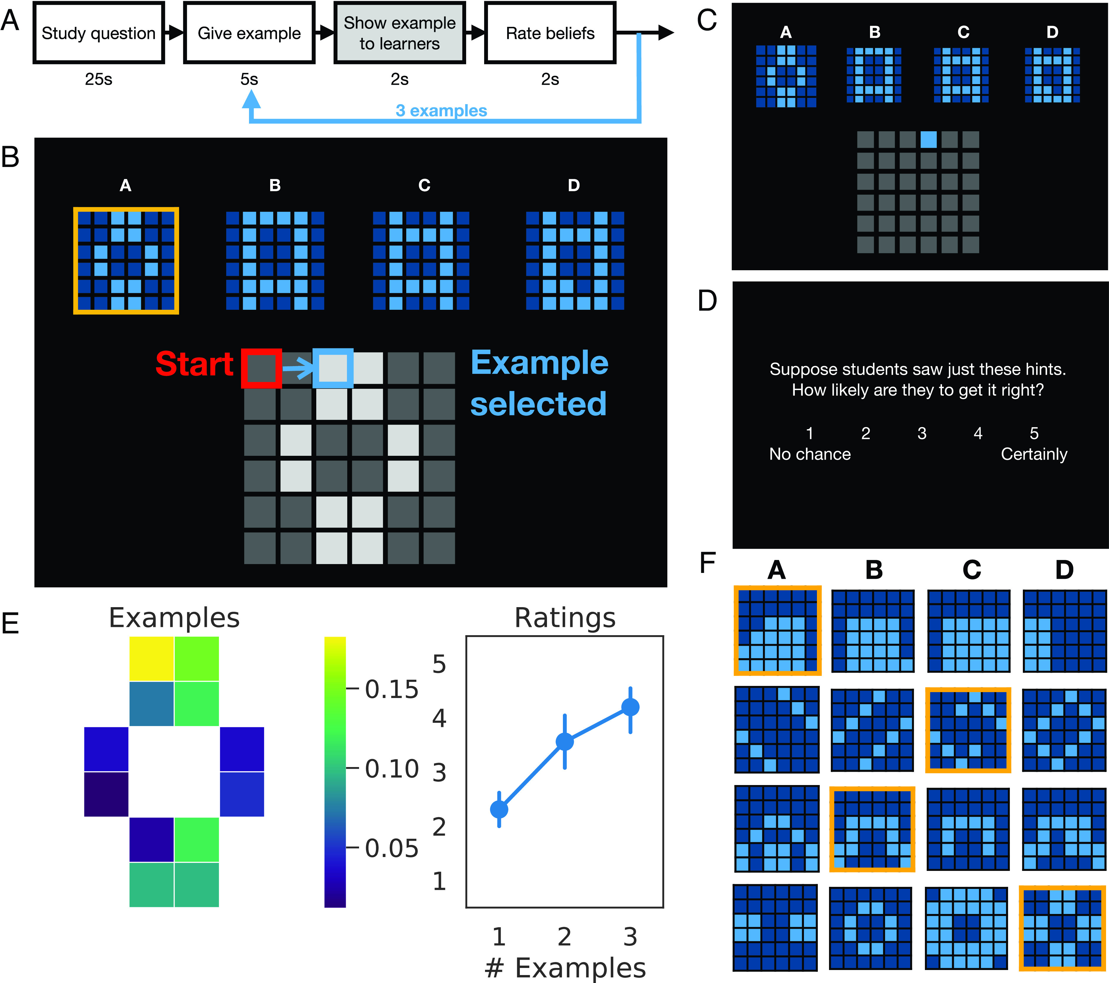
Experiment design & behavioral results. (A) Task structure and timing: At the start of each block, participants studied the question before being prompted to respond (“Study question”). Then, in each of three test trials, participants chose an example to provide to learners (“Give example”), saw the example presented from learners’ perspective (“Show example to learners”), and rated how likely learners would be to pick the correct answer, given the examples provided so far (“Rate beliefs”). (B) Choice screen: Participants could reveal to learners where the light blue squares were; these were highlighted in light gray on the canvas. Participants selected examples by moving a cursor; the cursor turned blue when participants navigated to a valid example. (C) In the critical event, participants saw the examples that they had selected so far as they would appear to learners. (D) Rating screen. (E) Behavioral results: Participants’ examples (Left) and trial-by-trial ratings (Right) for the question in panel B. The brightness of each cell shows the proportion of teachers who chose to reveal that square to learners. Error bars denote bootstrapped 95% CIs. (F) Other representative questions; see also SI Appendix, Fig. S1.

Finally, participants rated how likely learners would be to answer the question correctly, given the examples they had selected so far (Fig. 1D). Fig. 1E shows teachers’ examples and ratings for one representative question, and Fig. 1F shows a sampling of other multiple choice questions; average participant responses for these questions are shown in SI Appendix, Fig. S1. Participants taught learners how to answer 40 multiple-choice questions. These questions were designed to be sufficiently varied to prevent teachers from learning a simple strategy that would generalize across target concepts, such as touching opposite corners. Participants were told that the examples they selected would then be shown to other, future participants from across the United States.

Teachers Balance Communicative Costs against the Benefits to the Learner.

We modeled participants’ decisions about which examples to teach by defining a suite of models that select examples sequentially by balancing three values: the informational value to the learner, the movement costs to the teacher, and the teacher’s preferences (Fig. 2).

Fig. 2.

Schematic of computational models. (A) Literal and pedagogical learners: Here, the teacher selects an example to teach a learner how to answer a toy question with two 2 × 2 alternatives. The literal learner’s beliefs are uniformly distributed among the options that are consistent with the example provided. By contrast, the pedagogical learner favors option B, even though neither option has been definitively ruled out. Intuitively, the pedagogical learner’s beliefs are guided by an expectation of what the teacher could have shown; if the teacher had been trying to point them toward option A, they could have chosen the square on the top-right corner. (B) Augmenting learner models: The full model computes the utility of possible examples (light blue squares) based on three values: the informational value to the learner, the teacher’s speaker preferences, and the movement cost to the teacher. The bottom row shows each of these values for all possible examples in the multiple-choice question shown in Fig. 1; brighter cells have higher values.

In order to measure the informational value of an example to the learner, these models represent learners’ beliefs and select examples that will maximize their posterior belief in the correct answer. In information-theoretic terms, this is equivalent to minimizing the learner’s surprisal ($U_{\mathit{info}}=ln\left(P_L\left(h\right|d)\right)$; see also ref. 10). We defined three families of models, which differ in how they compute learners’ beliefs (Fig. 2A). First, pedagogical learner models assume that teachers and learners reason about each other recursively: Teachers select evidence that will maximize the learner’s belief in a concept ($P_T(d;h)\propto (P_L\left(h\right|d){)}^{{\omega }_{\mathit{info}}}$), while learners infer what concept the teacher is trying to teach them ($P_L\left(h\right|d)\propto P_T\left(d\right|h)$). ${\omega }_{\mathit{info}}$ is a free parameter that controls how strongly teachers choose examples that maximize learners’ beliefs; teachers tend to respond randomly as ${\omega }_{\mathit{info}}\to 0$, and to deterministically select the option that maximizes learners’ beliefs as ${\omega }_{\mathit{info}}\to \infty$. In principle, learners and teachers could reason recursively about each other indefinitely; in practice, this system of equations converges to a fixed point after a finite number of steps (SI Appendix, Fig. S2). This approach is often used in models of pedagogy (e.g., ref. 8). Second, literal learner models assume that learners’ beliefs are uniformly distributed across the options that are consistent with the examples provided; this model is equivalent to the one above, but stops after a single recursive step. This approach is often used in models of pragmatic language use, which assume that speakers say things that will be most informative to a listener who interprets them literally (e.g., ref. 13). Finally, as a baseline, we also included a family of belief-free models that do not use learners’ beliefs to select examples.

In addition to considering learners’ beliefs, teachers have little time to evaluate each question and move the cursor across the screen to select examples. Therefore, it is important to take into account that some examples may require more effort to select or may be more salient than others. For example, participants tended to choose examples that were closer together and closer to the contours of the target concept than one would predict if teachers solely acted to maximize the benefits to the learner (SI Appendix, Fig. S3). Each of the three families of models defined above contained models that incorporated teachers’ communicative costs and preferences into their decisions (Fig. 2B). We modeled the movement cost of an example ($C(d_t|d_{t-1})$) as the Manhattan distance between the starting point of the cursor and the example. The cursor started at a random corner of the canvas on the first trial of each question and on the location of the most recently selected example on subsequent trials. Finally, to account for teachers’ idiosyncratic preferences ($S(d_t)$), we assigned a higher weight to examples that had fewer light blue squares surrounding it. This weighting favors examples on the contours of the correct answer.

Put together, at time $t$, the utility of an example $d_t$ is defined as:

$$\begin{array}{c}U(d_t;h;\overline{\omega };d_{1..t-1})={\omega }_{\mathit{info}}·ln\left(P_L\left(h\right|d_{1..t})\right)\hfill \\ +{\omega }_{\mathit{cost}}·C\left(d_t\right|d_{t-1})+{\omega }_{\mathit{speaker}}·S\left(d_t\right),\hfill \end{array}$$ [1]

where $h$ is the target concept and $\overline{\omega }$ is a vector of coefficients that control the relative weighting of each of these values. Examples were selected probabilistically, in proportion to their utilities, using a softmax function ($P\left(x\right)=exp\left(U\left(x\right)\right)/{\mathrm{\Sigma }}_{x\text{'}}exp\left(U(x\text{'})\right)$.

We defined 12 models (Fig. 3A) that differed in how they represent learners’ beliefs (pedagogical, literal, and belief-free) and in whether they assign nonzero coefficients to the teacher’s movement costs and preferences. Each model makes distinct predictions about how teachers should select examples; SI Appendix, Fig. S4 shows model and parameter recovery results on simulated datasets. To select a model for fMRI analysis, we performed random-effects Bayesian model selection [(43); see SI Appendix, SI Methods for more details]. From this procedure, a clear winning model emerges: The most likely model in the population is one that selects examples to teach by considering the teacher’s preferences, the teacher’s movement costs, and the informational value to a learner who will interpret the examples literally (protected exceedance probability > 0.999; Fig. 3A). Additionally, models that considered the beliefs of a literal learner consistently provided the best fit to individual participants’ teaching behavior, compared to models that considered the beliefs of a pedagogical learner or models with no belief representations at all (SI Appendix, Fig. S4E). Thus, in the model-based fMRI analyses below, we use a literal learner model to predict learners’ posterior belief in the correct answer.

Fig. 3.

Model comparison & predictive checks. (A) Model comparison: The y axis shows distributions of model evidences, defined as −0.5*BIC, for each participant (44). Along the x axis, we considered three classes of models: pedagogical learner models (S_N), literal learner models (S₁), and those that included no belief representations at all (belief-free). Within each class of models, we defined alternative models by setting coefficients to 0; green cells denote nonzero coefficients in each model. (B–F) Predictive checks. (B) Examples chosen by a representative participant for the question on Fig. 1. The red square shows the starting point of the cursor on the first trial; the light blue squares show the examples selected by the participant, and the order in which they were selected. (C) Trial-by-trial predictions generated by the winning, literal-listener model (S₁: all ω > 0) and by (D–F) alternative models that consider only informational value, teacher preferences, and movement costs, respectively. The brightness of each square shows the model-predicted probability that the teacher will select that square on a particular trial; the white border shows which example the teacher actually selected.

Taking a closer look at this full model shows what each of these terms contributes to the model predictions (Fig. 3 B–F). Fig. 3B shows the examples selected by one teacher for the question shown in Fig. 1. The full model predicts that the teacher should choose examples that will uniquely identify the correct answer at t = 0 and t = 1, and choose a nearby example at t = 2 once all other options have been ruled out (Fig. 3C). A single term in our utility function could not have predicted this pattern. A model that considers only the informational value to the learner prioritizes examples that will uniquely identify the correct answer, but is indifferent between these examples (Fig. 3D). Conversely, a model that prefers only examples at the contours disprefers the examples selected by the teacher, and does not change its predictions after each trial (Fig. 3E). Finally, a model that considers only movement costs simply predicts that participants should pick the closest available example on each trial (Fig. 3F).

Teachers Accurately Predicted the Performance of an Independent Sample of Learners.

So far, our results suggest that teachers select examples by balancing the informational value to the learner against their own preferences and communicative costs. They also add to a growing body of evidence that teaching is supported by mentalizing: The informational value of a given example depends on the learner’s beliefs, and on how those beliefs will change with new examples. However, it is an open question whether teachers’ representations of learners are well calibrated. That is, what teachers think learners will believe does not necessarily correspond to what they actually believe. We addressed this question by testing an independent online sample of learners on the examples that teachers provided (N = 140; see Materials and Methods–Learner task).

Learners were assigned to a different teacher on each question, and they saw the examples that that teacher selected in sequence (Fig. 4A). After seeing each new example, learners rated the probability that each of the four drawings was the correct answer. Participants were told that these ratings would be used to distribute 100 “chips” to bet on the correct answer; the more chips they placed on the correct answer, the larger the bonus they would receive. We counterbalanced which teacher’s examples were assigned to each learner so that learners could receive examples from as many teachers as possible (mean: 27.7 teachers, range 23 to 28) and so that teachers could share their examples for each question with at least five learners (mean: 5 learners per teacher per question, range 5 to 6).

Fig. 4.

Learner behavior. An independent sample of learners was tested using the examples that teachers provided during the scanner task. (A) Task: Learners saw the examples provided by teachers in sequence. On each trial, they used sliders to place bets on the correct answer. (B) Learner performance: Overall, learners converged on the right answer as they received more examples (C) Relationship to teachers’ predictions: Teachers’ predictions about how likely learners would be to get each question right were correlated with learners' actual trial-by-trial performance. Error bars denote bootstrapped 95% CIs; the dotted line denotes chance performance.

Overall, learners tended to assign a higher probability to the correct answer as they received more examples (Fig. 4B; main effect of time: $\beta =0.03$, $t=4.751$, $P< 0.001$). While we observed substantial variation in how well learners performed on different questions, we did not observe much variation based on the teacher they were assigned to, suggesting that the examples that different teachers provided were of comparable quality (SI Appendix, Fig. S5). Our key analysis tested whether teachers’ predictions about how well learners would do corresponded with how they actually did, after adjusting for time and for random effects of teachers, learners, and questions (see Materials and methods for details). After adjusting for these factors, we found a close relationship between teachers’ predictions about how likely learners would be to answer correctly and learners’ belief in the correct answer (Fig. 4C; main effect of teachers’ predictions: $\beta =0.02$, $t=4.6$, $P< 0.001$; interaction between time and teachers’ predictions: β = 0.01, t = 7.2, P < 0.001). These results provide convergent evidence that teachers possessed a well-calibrated model of learners’ mental states.

Bilateral TPJ and Middle, Dorsal MPFC Track Trial-by-Trial Changes in Learners’ Beliefs.

Our behavioral results provide two lines of evidence that teachers represent learners’ beliefs when deciding what to teach. First, teachers’ examples were best explained by a model that maximizes the learner’s belief in the correct answer while taking the teacher’s communicative costs and preferences into account. Second, teachers’ trial-by-trial predictions about learners’ performance tracked the actual performance of an independent sample of learners. With this evidence in hand, we can now search for neural correlates of learners’ beliefs.

We examined two sets of regions of interest that have been implicated in processing social information (Fig. 5A). First, we functionally identified the mentalizing network within individual participants using an independent localizer task [(45, 46); see Localizer task, below] and hypothesis spaces drawn from a large sample of participants who were tested on the same localizer (SI Appendix, Fig. S6 and Table S1). Second, we defined ACCg anatomically as cytoarchitectonic area 24a/b (47, 48).

Fig. 5.

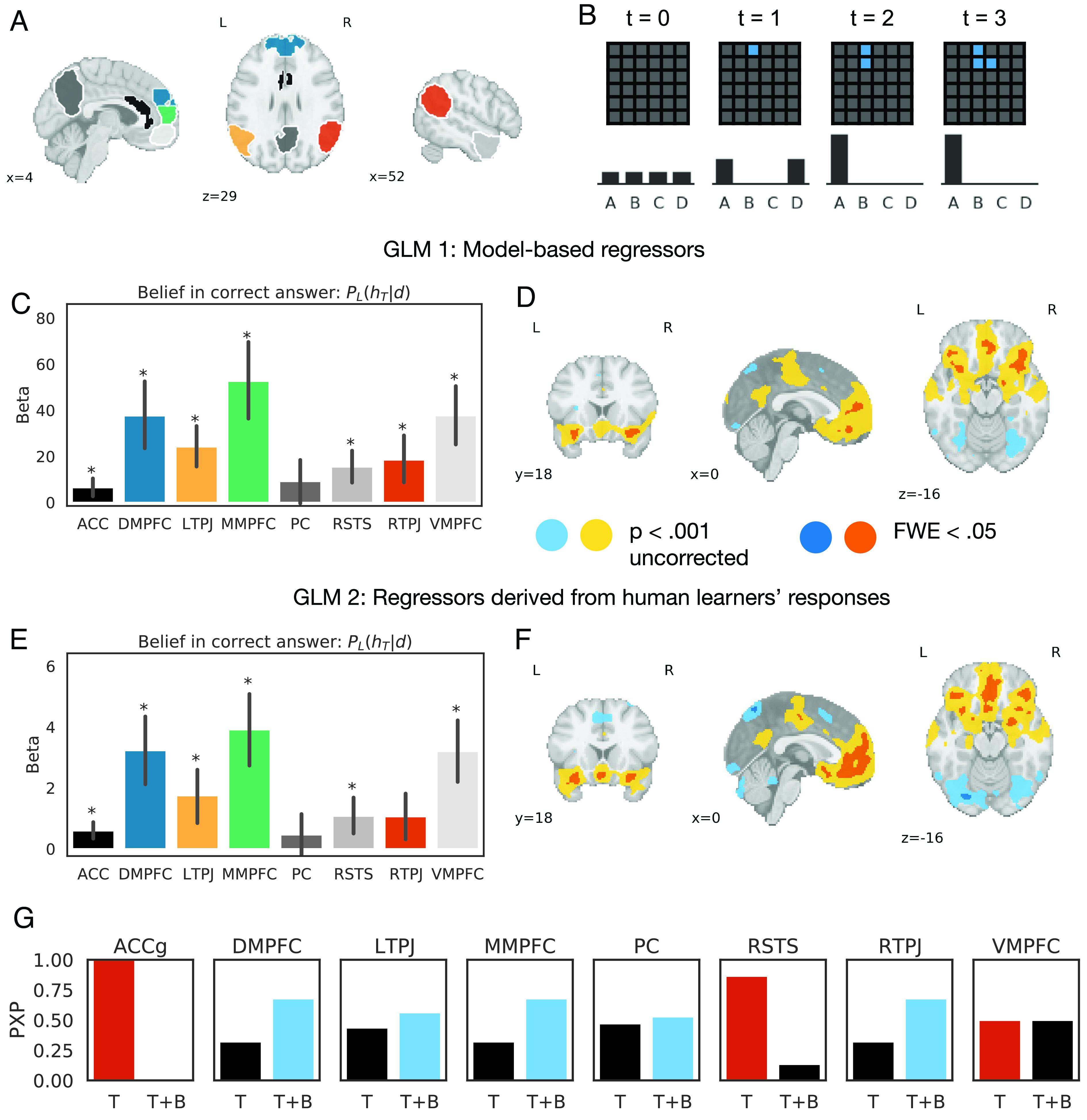
fMRI results. (A) Anatomical region of interest for anterior cingulate gyrus (black) and functionally defined regions within the mentalizing network from a representative participant (remaining colors). (B) Schematic of the literal listener model’s beliefs, given the examples provided by the participant in Fig. 3; note that “A” is the correct answer. (C and D) ROI and whole-brain results using model-based regressors (GLM 1). (C) Average activations across regions of interest. Error bars denote bootstrapped 95% CIs; asterisks mark significant activations after Bonferroni correction (one-sample t test, P < 0.05/8). (D) Thresholded whole-brain activations. Warm tones show significant activations in uncorrected statistical maps (yellow; P < 0.001, cluster extent > 10 voxels) and after family-wise error correction (orange; FWE < 0.05, cluster extent > 10 voxels). Cool tones show significant deactivations in uncorrected (light blue) and FWE-corrected (navy blue) maps. (E and F) ROI and whole-brain results using parametric regressors derived from human learners’ average responses (GLM 2). (G) Model comparison. We compared how well variability in activations in each ROI is explained by two GLMs: a control model that tracks the number of examples presented (Time, GLM 5), and a GLM that additionally includes parametric regressors for the learner’s belief and belief update (Time + Belief, GLM 6). The y axis shows protected exceedance probabilities for each GLM; red bars denote ROIs that were best fit by the control GLM, while blue bars denote ROIs that were best fit by the GLM that additionally tracks learners’ beliefs.

Within these regions of interest, we performed an ROI-based univariate analysis using a general linear model (GLM 1; see Materials & methods) with model-derived, trial-by-trial estimates of two quantities: learners’ posterior belief in the correct answer ($P_L(h_{\mathit{True}}|d_{1..t})$), and a belief update signal defined as the Kullback–Leibler divergence between learners’ belief distribution on successive trials ($D_{\mathit{KL}}\left(P_{L,t}\left|\right|P_{L,t-1}\right)$), following the modeling procedure in ref. 49 (Fig. 5B). Note that both regressors are derived from the beliefs of a literal learner model, based on the structure of the teaching problem and on the examples presented so far; they are not affected by free parameter values (e.g., ${\omega }_{\mathit{info}}$). After Bonferroni correction, all regions of interest except PC tracked learners’ posterior belief in the correct answer (Fig. 5C; all $ps< 0.05/8$). A post hoc whole-brain analysis suggests that this effect is largely localized within our a priori regions of interest; bilateral ventrolateral prefrontal cortex was the only region outside of our hypothesis space to survive multiple-comparisons correction (FWE < 0.05, cluster extent > 10; Fig. 5D). We obtained similar results using parametric regressors that were derived from human learners’ average bet allocations (GLM 2; Fig. 5 E and F) and using independent ROIs derived from Neurosynth (SI Appendix, Fig. S7).

We then tested whether activations within each of these regions could be explained by simpler task variables. The literal learner model’s belief in the correct answer increases monotonically, and is thus correlated with task variables such as the number of examples presented or the amount of time spent on a question (SI Appendix, Fig. S8). To test whether these variables can account for our findings, we used Bayesian model selection to compare two GLMs: a control GLM that merely tracks the number of examples presented (GLM 5), and a GLM that additionally tracks learners’ posterior belief and belief update, as in GLM 1 (GLM 6). Fig. 5G shows the results of this model comparison: Three ROIs—ACCg, RSTS, and VMPFC—were best explained by the control GLM, while activations in bilateral TPJ, MMPFC, and DMPFC were best explained by the GLM that additionally represents learners’ beliefs.

By contrast, evidence for neural correlates of belief updating was mixed. We did not find any regions where activity correlated positively with learners’ belief update. Instead, activity across several regions within the mentalizing network was negatively correlated with model-based estimates of learners’ belief update, and uncorrelated with regressors derived from human learners’ average belief update (SI Appendix, Fig. S9). We found similar results even after estimating each parametric regressor in a separate GLM, to account for correlations between regressors (GLM 3–4; SI Appendix, Figs. S10 and S11). Our results diverge from prior work, which has found that instructors vicariously represent learners’ prediction errors when providing feedback (26). We consider potential explanations for this discrepancy in the Discussion.

Put together, our results suggest that activity in mentalizing regions—namely DMPFC, LTPJ, MMPFC, and RTPJ—tracks the learners’ posterior belief in the correct answer, and that this result cannot be explained by simpler confounding variables. By contrast, we find comparably weaker evidence that these regions contribute to the representation of the learner’s belief update—that is, how much their beliefs have changed—at the same moment in time.

Discussion

Teaching enables humans to efficiently transfer knowledge. In the past, both computational and developmental studies of teaching have proposed that teaching relies on mentalizing—that is, on our ability to represent other people’s mental states, and to anticipate how those beliefs will change during teaching. Here, we examined the neural correlates of belief representations as people make decisions about what to teach. By modeling participants’ behavior, we find that teachers indeed choose examples that will maximize a learner’s belief in a target concept, while also taking their own preferences and communicative costs into account. Consistent with the idea that teachers represent and anticipate how learners’ beliefs will change, teachers’ trial-by-trial predictions about how well learners would do correlated with the actual performance of an independent sample of human learners. Using the computational model that best fits teachers’ behavior, we then examined how belief representations are neurally instantiated. We took a hypothesis-driven, ROI-based approach, examining eight regions that have been implicated in processing social information. Overall, activity in bilateral TPJ and dorsal and middle MPFC correlated with learners’ trial-by-trial beliefs in the correct answer; further, activity in these regions was best explained by a GLM that represented learners’ beliefs, compared to a control GLM that merely tracked the number of examples presented. A whole-brain analysis showed that this effect was largely localized within our regions of interest. Put together, our work ties computational theories of teaching to their neural instantiation, providing evidence that mental state representations within the mentalizing network play a role during teaching.

Our results suggest ways that existing models of teaching may be improved to better capture actual teaching behaviors. Pedagogy models are part of a broader suite of models of cooperative communication (10, 18)—the principles that guide good teaching also guide good communication in other domains, such as language. Our results suggest that we should take inspiration from a broader swath of models of communication to not only build normative theories of how teachers should select evidence, but also to identify what shortcuts they may take in doing so. In particular, our results suggest that teachers did not engage in computationally costly recursive mentalizing, but instead chose examples that would be most informative to a learner who interprets them literally—that is, one who rules out the options that are contradicted by the examples provided and is indifferent among the rest. Further, while teachers did provide information that was helpful to learners, this was not the only consideration that guided their decisions. The best-performing model considered not only the benefits to the learner, but also the motor costs of providing particular examples and the teacher’s idiosyncratic preference for examples along the contours of the target concept.

These discrepancies between idealized models of teaching and our participants’ teaching behavior echo recent trends in models of pragmatic language use. The models that best capture how people communicate through language tend to favor descriptions that will be most informative to a simple, literal learner and that are shorter, more typical, or more salient in context (13, 16, 50). It remains an open question why teachers opted for these shortcuts in our task. As illustrated in the toy problem in Fig. 2, recursive mentalizing can accelerate learning in cases where the examples available cannot definitively rule out alternative concepts. One possibility is that teachers’ behavior in our task reflects the rational use of limited cognitive resources (51, 52). For example, teachers may have opted for this strategy to avoid exhaustively performing inference over all possible examples (53, 54), or to ensure that their examples would be understood by a broad audience of learners of varying degrees of sophistication (55, 56). If this is the case, then we may expect teachers to adapt their strategy based on the computational demands of the task and the sophistication of the learner. For example, teachers may engage in recursive reasoning when they are faced with a particularly challenging problem where a literal learner cannot definitively rule out any concept, or when they are paired with a sophisticated pedagogical learner that quickly converges on an answer.

Our results raise further questions about the neural computations that guide teaching behaviors. For instance, we found a univariate neural response within the mentalizing network that tracked teachers’ estimates of the degree to which learners held a true belief about the correct answer. Our results contrast with prior work on the mentalizing network, which has tended to find reduced neural activation in response to predictable descriptions of mental states, relative to unexpected ones (57) and relatively great activation in response to false beliefs, relative to true beliefs (58). Other work finds multivariate neural patterns in the mentalizing network that are associated with the specific contents of mental state representations (34, 59), rather than univariate responses. Here, however, we find a strong correlate of true belief. This result may reflect the goal-directed structure of our task, in that participants’ goal was to bring about a specific true belief in the minds of learners. This hints at an intriguing integration of mentalizing and planning that may be fundamental to the power of human pedagogy (60).

Unexpectedly, although we found neural correlates of teachers’ representations of learners’ beliefs, we did not find the hypothesized neural correlates of the learners’ updating process. While prior research suggests that teachers show a neural response proportional to the magnitude of the update they impute to learners (26), here we find modest evidence for the inverse relationship. This result demands further study. Though it is natural to assume that teachers would maintain a representation of learners’ belief updates, it is possible that the specific period of time that we modeled—the moment when teachers observe the learner receiving their message—does not coincide with updating. That is, teachers may project updates when they select examples, obviating the need to recompute them upon seeing those examples presented. This is a notable dimension on which our study differs from that of ref. 26; future work may explore these differences by employing tasks where teachers observe how learners respond to their examples sequentially, in a real-time social interaction.

Finally, while we have identified an important commonality in how learners’ beliefs are represented in bilateral TPJ and MPFC, it is an open question how the computations implemented by each of these regions may differ from one another. TPJ and MPFC are functionally connected (61, 62) and are engaged in a variety of mentalizing tasks, including false belief processing, trait attributions, and strategic decision-making in games (63). However, while these regions tend to work in concert, past work also suggests that they may implement different computations. For example, in the domain of strategic decision-making, TPJ activity tracks outcomes when playing competitive games against another human, while MPFC activity reflects the deployment of particular behavioral strategies regardless of whether they are used against a human or a computer (39). These results raise questions about whether TPJ and MPFC also play dissociable computational roles in teaching, and to what extent these computations overlap with other mentalizing tasks or with domain-general functions such as planning (64). Future work may address this question through the use of nonsocial controls.

Past work on the neural bases of social cognition has largely examined the computations that underlie learning from others; this work has emphasized continuities between the computational principles and neural architectures that govern social learning and learning through firsthand experience with the environment (65–67). By contrast, less is known about the neural computations that support teaching (but see ref. 26), and still less is known about the extent to which these computations draw on specialized mechanisms for social cognition. The current work takes a different approach: Rather than probing these continuities, we instead ask whether teachers represent learners’ mental states as they decide what to teach—a distinctively social process. Overall, we find that teachers represent learners’ beliefs as they decide what to teach, and these beliefs are represented in several regions that play specialized roles in processing social information. Our work lays an empirical and conceptual foundation for understanding the neural architectures that make human teaching efficient and powerful (68).

Materials and Methods

Participants.

Twenty-eight participants (17 female, M(SD) age = 22.1(4.0) were recruited from the Cambridge, MA community. Participants were healthy, aged 18 to 40, right-handed, with normal or corrected-to-normal vision; they received $80 for their participation plus a performance bonus. Participants gave fully informed, written consent for the project, which was approved by the Institutional Review Board at Harvard University.

An additional two participants were excluded from analysis. Both participants had at least four runs with excessive motion (i.e., >2 mm translational motion or >2° rotational motion), including both runs of an independent localizer task (see Localizer task, below). No participants in the final sample had runs with excessive motion.

Scanner Task.

In the main scanner task, participants selected examples to teach learners how to answer multiple-choice questions. Each question was composed of four 6 × 6 pixel drawings of light blue figures on a dark blue background. Participants were told that learners would receive a reward if they selected one of these options (the “correct answer”). Fig. 1A shows a representative question; the correct answer was highlighted with a gold border. Additional multiple-choice questions are shown in SI Appendix, Fig. S1.

Fig. 1B shows the task structure. Participants provided up to three examples per question. Each question began with a 3 to 7 s jittered fixation period. Teachers then looked at the question for 25 s (“Study question”) before being prompted to choose examples.

Teachers completed three test trials for each question, and each trial was composed of three phases. First, participants selected examples to communicate to future learners by revealing parts of the correct answer on the “canvas” (“Give example”; 5 s), a dark gray, 6 × 6 grid placed below the four choice alternatives. Participants could only reveal the locations of the light blue squares to learners; to borrow terminology from past work (8, 42), this constraint is analogous to only providing positive examples that are contained within the target concept. Available examples were highlighted in light gray on the canvas. Participants selected examples by moving a cursor using a button box. At the start of each question, the cursor appeared in one of the four corners of the screen; the cursor’s starting location was counterbalanced within each run. The cursor appeared red when placed over an invalid example (i.e., a dark square or a previously selected example), blue when placed over a valid example, and gold once the participant confirmed their choice. After participants selected their first example, the cursor instead started off in the location of the most recently selected example.

Next, participants saw how the examples they selected would look to learners (“Show example to learners”; 2 s). All parametric regressors were modeled during this event (see fMRI analysis). Participants saw a fixation cross for .75 to 2.5 s and a prompt for 1 s (“Here's what students would see:”) before the display was revealed from the learner's perspective (Fig. 1C). In this display, the correct answer was not highlighted among the choice alternatives, and the canvas was a uniform shade of dark gray. Selected examples appeared as light blue squares on the canvas.

Finally, participants rated how likely learners would be to answer the question correctly, given the examples provided so far (“Rate beliefs”; 2 s). Participants answered this question on a five-point Likert scale, where a response of one indicated that there was “No chance” that learners would get the question right, and a response of five indicated that learners would “Certainly” get it right. Participants then saw a fixation cross for .75 to 2.5 s before the next trial. Participants taught 40 questions total, spread over 10 runs.

Localizer Task.

We used an independent functional localizer task to identify participant-specific mentalizing regions (45). Participants read short stories describing a character’s mental state (Belief condition) or closely matched but nonmental representations, such as books, maps, and photographs (Physical condition). Participants completed two runs of this task, each containing five Belief trials and five Physical trials.

Learner Task.

Participants.

A total of 140 participants were recruited on Amazon Mechanical Turk. Participants were paid $2 and a performance bonus of up to $5 (median time to completion: 25 min, median hourly pay: $10.64). Participants gave fully informed, written consent for the project, which was approved by the Institutional Review Board at Harvard University.

Procedure.

Teachers' examples were presented, one by one, on a canvas in the top half of the screen. The canvas was a gray 6 × 6 array; the examples selected by the teacher were revealed to participants as black squares on the canvas. In the bottom half, learners were shown four possible answers to the question; each option was depicted as a pixel drawing of a black figure on a white background. Each option had a slider beneath it, which learners could use to place bets; the more participants moved a slider to the right, the more strongly they believed that that option was the correct answer. At the end of each question, participants received a small bonus that was proportional to how much they had bet on the correct answer.

We did not present teachers’ hints to learners if they failed to provide at least two hints during the response periods. Seven teachers had one question excluded from this study, and one teacher had two questions excluded.

Statistical analysis.

We converted participants’ bet allocations into belief distributions by rescaling them to sum to one. From these belief distributions, we then measured learners’ average self-reported belief in the correct answer. In our key analysis, we used the lme4 and lmerTest packages in R to estimate a mixed-effects linear model that predicted learners’ posterior belief in the correct answer as a function of time (i.e., how many examples had been presented, coded as a continuous variable), teachers’ predictions about how likely students would be to answer correctly (ranging from 1 = no chance to 5 = certainly, and also coded as a continuous variable), and the interaction between the two (belief_in_true ~ time*teacher_rating + (1|problem) + (1|learner) + (1|teacher)). Learners, teachers, and problems were included as random intercepts.

fMRI Analysis.

ROI analyses.

Mentalizing network.

We identified participant-specific mentalizing regions by combining functional data from the localizer task with hypothesis spaces derived from activations from a large sample of adults tested on the same localizer (46). Each condition (Belief, Physical) was modeled as a 14 s boxcar spanning the length of the narrative and question. Within each subject, we contrasted responses to Belief > Physical (t-contrast, P < 0.001 uncorrected, minimum cluster size: 10) to identify ROIs. Using the resulting statistical maps, we defined each ROI by extracting the cluster containing the peak voxel within each region and by masking each cluster using that region’s hypothesis space. When no suprathreshold voxels were found within a hypothesis space, we repeated the search at P < 0.01 and P < 0.05. Finally, we masked each ROI using its hypothesis space so that there was no overlap in the voxels defined in each ROI. SI Appendix, Fig. S6 shows ROI hypothesis spaces and the distribution of ROI locations and extents in our sample; SI Appendix, Table S1 shows average peak voxel locations and ROI extents.

We also defined independent mentalizing ROIs using Neurosynth (69). We retrieved a statistical map testing for the presence of a nonzero association between voxel activation and the use of the term “mentalizing” (N = 151 studies, 6,824 activations), thresholded to correct for multiple comparisons (FDR = 0.01). This association test identifies activations that occur more consistently in studies that include the term “mentalizing” than in studies that do not. We then binarized this statistical map and split it into clusters. This analysis identified seven clusters of activations in cortex and 2 clusters in the cerebellum (SI Appendix, Fig. S7); cerebellar clusters were excluded from analysis.

ACCg.

We identified ACCg anatomically as bilateral cytoarchitectonic areas 24a/b in ref. 48 (http://www.rbmars.dds.nl/CBPatlases.htm).

GLM.

We defined four GLMs based on the winning behavioral model (GLM 1, 3 to 4, 6), one GLM based on average responses in the learner task (GLM 2), and one control GLM that contained a single parametric regressor tracking the number of examples presented (GLM 5). All GLMs included six motion regressors, nuisance impulse regressors marking each time participants pressed a button, and boxcar regressors spanning each phase of a trial (Fig. 1A). In addition, for all GLMs, we defined parametric regressors during events where the example was presented to the teacher from the learners’ perspective (i.e., the “Show example to learners” event in Fig. 1A). These GLMs differed in which parametric regressors were included during this event.

Model-based GLM (GLM 1).

The goal of this GLM was to identify neural signals that track trial-by-trial fluctuations in the learner’s beliefs and belief update. GLM 1 included parametric regressors for model-based, trial-by-trial estimates of two quantities: the learner’s posterior belief in the correct answer, based on the evidence provided ($P_L\left(h\right|d_{1..t})$), and the learner’s belief update. We defined the latter regressor as the Kullback–Leibler divergence between the learner’s posterior belief distribution after the current example was presented and their prior beliefs ($D_{\mathit{KL}}(P_t||P_{t-1})$). On the first trial, we computed this belief update by comparing the learner’s posterior belief against a uniform prior.

Empirical GLM (GLM 2).

The goal of this GLM was to identify regions that track learners’ beliefs in a way that is independent of our model implementation. As above, GLM 4 included parametric regressors for learners’ posterior belief and belief update. However, in GLM 4, these quantities were not estimated from the winning model, but rather from average responses on the learner task. Recall that, for each question, we presented the teacher’s examples to an average of five different learners, and each learner updated their bets as the teacher’s examples were presented sequentially. We converted learners’ bets into probability distributions by averaging over the bets provided by learners in response to a particular example, and then rescaling this average bet to sum to one. Measures of posterior belief and belief update were then defined from empirically derived probability distributions using the procedure described above.

Estimating model-based regressors in separate GLMs (GLM 3 to 4).

These GLMs estimated the effects of learners’ posterior belief (GLM 3) and belief update (GLM 4) in separate models, using the same model predictions used to generate GLM 1.

Control GLMs (GLM 5–6).

These GLMs were used to test whether activations found in each ROI could be explained by simpler confounding variables, namely the number of examples presented. Both GLMs included a parametric regressor that tracked the number of examples presented; GLM 6 contained additional parametric regressors that tracked model-based estimates of learners’ posterior belief in the correct answer and belief update, as in GLM 1.

Statistical analysis.

We computed the average activity across a region of interest for a given participant by averaging beta-values across all voxels contained within that participant’s ROI mask. We then tested whether each of these regions reliably tracked learners’ posterior belief and belief update by averaging across average region-wide activities for each participant and conducting a one-sample t test against 0; we report Bonferroni–corrected results in Fig. 5 (P < 0.05/8). In addition, we compared these ROI-based results to activations across the whole brain at two different statistical thresholds (P < 0.001 uncorrected and FWE < 0.05; cluster extent > 10).

For GLM 5 to 6, we additionally used Bayesian model selection to compare which GLM best captures variability in activations within each ROI (43). Using the ccnl-fmri package (https://github.com/sjgershm/ccnl-fmri), we used each ROI to mask statistical maps of individual participants’ estimated residual variance, and then used residual variance to compute the BIC of a given GLM within that ROI. The BIC reflects how closely the GLM matches the neural activity within a given ROI, while adding a penalty based on the number of regressors in the GLM to account for overfitting. Following our behavioral model comparison procedure, model evidences were approximated as −0.5*BIC (44) and used to estimate the protected exceedance probabilities for each GLM.

Supplementary Material

Appendix 01 (PDF)

Data, Materials, and Software Availability

Behavioral data, unthresholded statistical maps, task code and other materials, analysis code data have been deposited in Open Science Framework (DOI https://doi.org/10.17605/OSF.IO/SP5TC) (70).

References

- 1.Kline M. A., Boyd R., Henrich J., Teaching and the life history of cultural transmission in Fijian villages. Hum. Nat. 24, 351–374 (2013). [DOI] [PubMed] [Google Scholar]
- 2.Rogoff B., Paradise R., Arauz R. M., Correa-Chavez M., Angelillo C., Firsthand learning through intent participation. Annu. Rev. Psychol. 54, 175–203 (2003). [DOI] [PubMed] [Google Scholar]
- 3.Csibra G., Gergely G., Natural pedagogy. Trends Cogn. Sci. 13, 148–153 (2009). [DOI] [PubMed] [Google Scholar]
- 4.Legare C. H., The development of cumulative cultural learning. Annu. Rev. Dev. Psychol. 1, 119–147 (2019). [DOI] [PMC free article] [PubMed] [Google Scholar]
- 5.Gweon H., Inferential social learning: Cognitive foundations of human social learning and teaching. Trends Cogn. Sci. 25, 896–910 (2021). [DOI] [PubMed] [Google Scholar]
- 6.Csibra G., Teachers in the wild. Trends Cogn. Sci. 11, 95–96 (2007). [DOI] [PubMed] [Google Scholar]
- 7.Hoppitt W. J. E., et al. , Lessons from animal teaching. Trends Ecol. Evol. 23, 486–493 (2008). [DOI] [PubMed] [Google Scholar]
- 8.Shafto P., Goodman N. D., Griffiths T. L., A rational account of pedagogical reasoning: Teaching by, and learning from, examples. Cogn. Psychol. 71, 55–89 (2014). [DOI] [PubMed] [Google Scholar]
- 9.Wang J., Wang P., Shafto P., Sequential cooperative bayesian inference. arXiv [Preprint] (2020). 10.48550/arXiv.2002.05706 (Accessed 21 March 2023). [DOI]
- 10.Shafto P., Wang J., Wang P., Cooperative communication as belief transport. Trends Cogn. Sci. 25, 826–828 (2021). [DOI] [PubMed] [Google Scholar]
- 11.Liszkowski U., Carpenter M., Tomasello M., Twelve-month-olds communicate helpfully and appropriately for knowledgeable and ignorant partners. Cognition 108, 732–739 (2008). [DOI] [PubMed] [Google Scholar]
- 12.Bridgers S., Jara-Ettinger J., Gweon H., Young children consider the expected utility of others’ learning to decide what to teach. Nat. Hum. Behav. 4, 144–152 (2020). [DOI] [PubMed] [Google Scholar]
- 13.Frank M. C., Goodman N. D., Predicting pragmatic reasoning in language games. Science 336, 998 (2012). [DOI] [PubMed] [Google Scholar]
- 14.Ho M. K., Cushman F., Littman M. L., Austerweil J. L., Communication in action: Planning and interpreting communicative demonstrations. J. Exp. Psychol. Gen. 150, 2246–2272 (2021). [DOI] [PubMed] [Google Scholar]
- 15.Gweon H., Shafto P., Schulz L., Development of children’s sensitivity to overinformativeness in learning and teaching. Dev. Psychol. 54, 2113–2125 (2018). [DOI] [PubMed] [Google Scholar]
- 16.Degen J., Hawkins R. D., Graf C., Kreiss E., Goodman N. D., When redundancy is useful: A bayesian approach to “overinformative” referring expressions. Psychol. Rev. 127, 591–621 (2020). [DOI] [PubMed] [Google Scholar]
- 17.Bass I., et al. , The effects of information utility and teachers’ knowledge on evaluations of under-informative pedagogy across development. Cognition 222, 104999 (2022). [DOI] [PubMed] [Google Scholar]
- 18.Wang P., Wang J., Paranamana P., Shafto P., A mathematical theory of cooperative communication. arXiv [Preprint] (2019). 10.48550/arXiv.1910.02822 (Accessed 21 March 2023). [DOI]
- 19.Yoon E. J., Frank M. C., Tessler M. H., Goodman N. D., Polite speech emerges from competing social goals. Open Mind (Camb.) 4, 71–87 (2018), 10.31234/osf.io/67ne8. [DOI] [PMC free article] [PubMed] [Google Scholar]
- 20.Behrens T. E. J., Hunt L. T., Woolrich M. W., Rushworth M. F. S., Associative learning of social value. Nature 456, 245–249 (2008). [DOI] [PMC free article] [PubMed] [Google Scholar]
- 21.Burke C. J., Tobler P. N., Baddeley M., Schultz W., Neural mechanisms of observational learning. Proc. Natl. Acad. Sci. U.S.A. 107, 14431–14436 (2010). [DOI] [PMC free article] [PubMed] [Google Scholar]
- 22.Campbell-Meiklejohn D., Simonsen A., Frith C. D., Daw N. D., Independent neural computation of value from other people’s confidence. J. Neurosci. 37, 673–684 (2017). [DOI] [PMC free article] [PubMed] [Google Scholar]
- 23.Hill M. R., Boorman E. D., Fried I., Observational learning computations in neurons of the human anterior cingulate cortex. Nat. Commun. 7, 12722 (2016). [DOI] [PMC free article] [PubMed] [Google Scholar]
- 24.Zhang L., Gläscher J., A brain network supporting social influences in human decision-making. Sci. Adv. 6, eabb4159 (2020). [DOI] [PMC free article] [PubMed] [Google Scholar]
- 25.Diaconescu A. O., et al. , Neural arbitration between social and individual learning systems. Elife 9, e54051 (2020). [DOI] [PMC free article] [PubMed] [Google Scholar]
- 26.Apps M. A. J., Lesage E., Ramnani N., Vicarious reinforcement learning signals when instructing others. J. Neurosci. 35, 2904–2913 (2015). [DOI] [PMC free article] [PubMed] [Google Scholar]
- 27.Frith C. D., Frith U., Mechanisms of social cognition. Annu. Rev. Psychol. 63, 287–313 (2012). [DOI] [PubMed] [Google Scholar]
- 28.Van Overwalle F., Social cognition and the brain: A meta-analysis. Hum. Brain Mapp. 30, 829–858 (2009). [DOI] [PMC free article] [PubMed] [Google Scholar]
- 29.Richardson H., Lisandrelli G., Riobueno-Naylor A., Saxe R., Development of the social brain from age three to twelve years. Nat. Commun. 9, 1027 (2018). [DOI] [PMC free article] [PubMed] [Google Scholar]
- 30.Fletcher P. C., et al. , Other minds in the brain: A functional imaging study of “theory of mind” in story comprehension. Cognition 57, 109–128 (1995). [DOI] [PubMed] [Google Scholar]
- 31.Saxe R., Kanwisher N., People thinking about thinking people: The role of the temporo-parietal junction in “theory of mind”. Neuroimage 19, 1835–1842 (2003). [DOI] [PubMed] [Google Scholar]
- 32.Brunet E., Sarfati Y., Hardy-Baylé M. C., Decety J., A PET investigation of the attribution of intentions with a nonverbal task. Neuroimage 11, 157–166 (2000). [DOI] [PubMed] [Google Scholar]
- 33.Koster-Hale J., Saxe R., Dungan J., Young L. L., Decoding moral judgments from neural representations of intentions. Proc. Natl. Acad. Sci. U.S.A. 110, 5648–5653 (2013). [DOI] [PMC free article] [PubMed] [Google Scholar]
- 34.Koster-Hale J., et al. , Mentalizing regions represent distributed, continuous, and abstract dimensions of others’ beliefs. Neuroimage 161, 9–18 (2017). [DOI] [PMC free article] [PubMed] [Google Scholar]
- 35.Jamali M., et al. , Single-neuronal predictions of others’ beliefs in humans. Nature 591, 610–614 (2021), 10.1038/s41586-021-03184-0. [DOI] [PMC free article] [PubMed] [Google Scholar]
- 36.Coricelli G., Nagel R., Neural correlates of depth of strategic reasoning in medial prefrontal cortex. Proc. Natl. Acad. Sci. U.S.A. 106, 9163–9168 (2009). [DOI] [PMC free article] [PubMed] [Google Scholar]
- 37.Hampton A. N., Bossaerts P., O’Doherty J. P., Neural correlates of mentalizing-related computations during strategic interactions in humans. Proc. Natl. Acad. Sci. U.S.A. 105, 6741–6746 (2008). [DOI] [PMC free article] [PubMed] [Google Scholar]
- 38.Hill C. A., et al. , A causal account of the brain network computations underlying strategic social behavior. Nat. Neurosci. 20, 1142–1149 (2017). [DOI] [PubMed] [Google Scholar]
- 39.Konovalov A., Hill C., Daunizeau J., Ruff C. C., Dissecting functional contributions of the social brain to strategic behavior. Neuron 109, 3323–3337.e5 (2021). [DOI] [PubMed] [Google Scholar]
- 40.Apps M. A. J., Ramnani N., The anterior cingulate gyrus signals the net value of others’ rewards. J. Neurosci. 34, 6190–6200 (2014). [DOI] [PMC free article] [PubMed] [Google Scholar]
- 41.Lockwood P. L., et al. , Neural mechanisms for learning self and other ownership. Nat. Commun. 9, 4747 (2018). [DOI] [PMC free article] [PubMed] [Google Scholar]
- 42.Avrahami J., et al. , Teaching by examples: Implications for the process of category acquisition. Q. J. Exp. Psychol. Sect. A 50, 586–606 (1997). [Google Scholar]
- 43.Rigoux L., Stephan K. E., Friston K. J., Daunizeau J., Bayesian model selection for group studies - Revisited. Neuroimage 84, 971–985 (2014). [DOI] [PubMed] [Google Scholar]
- 44.Bishop C. M., Pattern Recognition and Machine Learning (Springer, New York, 2006), (August 18, 2022). [Google Scholar]
- 45.Dodell-Feder D., Koster-Hale J., Bedny M., Saxe R., fMRI item analysis in a theory of mind task. Neuroimage 55, 705–712 (2011). [DOI] [PubMed] [Google Scholar]
- 46.Dufour N., et al. , Similar brain activation during false belief tasks in a large sample of adults with and without autism. PLoS One 8, e75468 (2013). [DOI] [PMC free article] [PubMed] [Google Scholar]
- 47.Apps M. A. J., Rushworth M. F. S., Chang S. W. C., The anterior cingulate gyrus and social cognition: Tracking the motivation of others. Neuron 90, 692–707 (2016). [DOI] [PMC free article] [PubMed] [Google Scholar]
- 48.Neubert F.-X., Mars R. B., Sallet J., Rushworth M. F. S., Connectivity reveals relationship of brain areas for reward-guided learning and decision making in human and monkey frontal cortex. Proc. Natl. Acad. Sci. U.S.A. 112, E2695–E2704 (2015). [DOI] [PMC free article] [PubMed] [Google Scholar]
- 49.Tomov M. S., Dorfman H. M., Gershman S. J., Neural computations underlying causal structure learning. J. Neurosci. 38, 7143–7157 (2018). [DOI] [PMC free article] [PubMed] [Google Scholar]
- 50.Qing C., Franke M., "Variations on a bayesian theme: Comparing bayesian models of referential reasoning" in Bayesian Natural Language Semantics and Pragmatics, Zeevat H., Schmitz H.-C., Eds. (Springer, 2015). [Google Scholar]
- 51.Gershman S. J., Horvitz E. J., Tenenbaum J. B., Computational rationality: A converging paradigm for intelligence in brains, minds, and machines. Science 349, 273–278 (2015). [DOI] [PubMed] [Google Scholar]
- 52.Lieder F., Griffiths T. L., Resource-rational analysis: Understanding human cognition as the optimal use of limited computational resources. Behav. Brain Sci. 43, e1 (2019). [DOI] [PubMed] [Google Scholar]
- 53.White J., Mu J., Goodman N. D., Learning to refer informatively by amortizing pragmatic reasoning. arXiv [Preprint] (2020). 10.48550/arXiv.2006.00418 (Accessed 21 March 2023). [DOI]
- 54.Wu C. M., Vélez N., Cushman F. A., “Representational exchange in human social learning: Balancing efficiency and flexibility” in The Drive for Knowledge: The Science of Human Information-Seeking, Dezza I.C., Schulz E., Wu C.M., Eds. (Cambridge University Press, 2022). [Google Scholar]
- 55.Hawkins R. D., Gweon H., Goodman N. D., The division of labor in communication: Speakers help listeners account for asymmetries in visual perspective. Cogn. Sci. 45, e12926 (2021). [DOI] [PubMed] [Google Scholar]
- 56.Frank M. C., Liu L., Modeling classroom teaching as optimal communication (2018). 10.31234/osf.io/bucqx (Accessed 21 March 2023). [DOI]
- 57.Koster-Hale J., Saxe R., Theory of mind: A neural prediction problem. Neuron 79, 836–848 (2013). [DOI] [PMC free article] [PubMed] [Google Scholar]
- 58.Sommer M., et al. , Neural correlates of true and false belief reasoning. Neuroimage 35, 1378–1384 (2007). [DOI] [PubMed] [Google Scholar]
- 59.Koster-Hale J., Bedny M., Saxe R., Thinking about seeing: Perceptual sources of knowledge are encoded in the theory of mind brain regions of sighted and blind adults. Cognition 133, 65–78 (2014). [DOI] [PMC free article] [PubMed] [Google Scholar]
- 60.Ho M. K., Saxe R., Cushman F., Planning with theory of mind. Trends Cogn. Sci. 26, 959–971 (2022). [DOI] [PubMed] [Google Scholar]
- 61.Mars R., et al. , On the relationship between the “default mode network” and the “social brain”. Front. Hum. Neurosci. 6, 189 (2012). [DOI] [PMC free article] [PubMed] [Google Scholar]
- 62.Sallet J., et al. , The organization of dorsal frontal cortex in humans and macaques. J. Neurosci. 33, 12255–12274 (2013). [DOI] [PMC free article] [PubMed] [Google Scholar]
- 63.Schurz M., Radua J., Aichhorn M., Richlan F., Perner J., Fractionating theory of mind: A meta-analysis of functional brain imaging studies. Neurosci. Biobehav. Rev. 42, 9–34 (2014). [DOI] [PubMed] [Google Scholar]
- 64.Lockwood P. L., Apps M. A. J., Chang S. W. C., Is there a “Social” Brain? Implementations and algorithms. Trends Cogn. Sci. 24, 802–813 (2020), 10.1016/j.tics.2020.06.011. [DOI] [PMC free article] [PubMed] [Google Scholar]
- 65.Behrens T. E. J., Hunt L. T., Rushworth M. F. S., The computation of social behavior. Science 324, 1160–1164 (2009). [DOI] [PubMed] [Google Scholar]
- 66.Li J., Delgado M. R., Phelps E. A., How instructed knowledge modulates the neural systems of reward learning. Proc. Natl. Acad. Sci. U.S.A. 108, 55–60 (2011). [DOI] [PMC free article] [PubMed] [Google Scholar]
- 67.Olsson A., Knapska E., Lindström B., The neural and computational systems of social learning. Nat. Rev. Neurosci. 21, 197–212 (2020). [DOI] [PubMed] [Google Scholar]
- 68.Vélez N., Gweon H., Learning from other minds: An optimistic critique of reinforcement learning models of social learning. Curr. Opin. Behav. Sci. 38, 110–115 (2021). [DOI] [PMC free article] [PubMed] [Google Scholar]
- 69.Yarkoni T., Poldrack R. A., Nichols T. E., Van Essen D. C., Wager T. D., Large-scale automated synthesis of human functional neuroimaging data. Nat. Methods 8, 665–670 (2011). [DOI] [PMC free article] [PubMed] [Google Scholar]
- 70.Vélez N., et al. , Teachers recruit mentalizing regions to represent learners' beliefs. Open Science Framework. 10.17605/OSF.IO/SP5TC. Deposited 24 August 2022. [DOI] [PMC free article] [PubMed]
Associated Data
This section collects any data citations, data availability statements, or supplementary materials included in this article.
Supplementary Materials