

Abstract
In this study, based on automatic control and image processing, a high-throughput and low-cost maize ear traits scorer (METS) was developed for the automatic measurement of 34 maize ear traits. In total, 813 maize ears were measured using METS, and the results showed that the square of the correlation coefficient (R2) of the manual measurements versus the automatic measurements for ear length, ear diameter, and kernel thickness were 0.96, 0.79, and 0.85, respectively. These maize ear traits could be used to classify the type, and the results showed that the classification accuracy of the support vector machine (SVM) model for the test set was better than that of the random forest (RF) model. In addition, the general applicability of the image analysis pipeline was also demonstrated on other independent maize ear phenotyping platforms. In conclusion, equipped with image processing and automatic control technologies, we have developed a high-throughput method for maize ear scoring, which could be popularized in maize functional genetics, genomics, and breeding applications.
Supplementary Information
The online version contains supplementary material available at 10.1007/s11032-021-01205-4.
Keywords: Maize ear traits, High-throughput method, Image processing, Support vector machine (SVM), Automatic measurement
Introduction
Maize (Zea mays L.) is one of the most important food and feed crops in the world (Chen et al. 2014). Maize ear traits, which include seed distribution, seed quantity, seed size, ear size, and ear shape, are important traits for genetic breeding research, as well as for physiological and ecological cultivation research (Yang et al. 2010; Liu et al. 2020). Currently, maize ear traits are mainly measured manually, which is time-consuming, tedious, and vulnerable to human error (Li et al. 2014). Thus, it is necessary to develop a high-throughput phenotyping machine to extract ear traits automatically.
In recent years, the morphological characteristics of agricultural products have been investigated and extracted by image analysis, which is more objective, automatic, and higher throughput than previous methods (Wu et al. 2020). Dubey et al. applied 45 morphological characteristics (such as shape, size, and color) to recognize wheat seed varieties (Dubey et al. 2006). Mebatsion et al. (2013) classified 5-grain varieties using morphological characteristics and color features. They extracted the Fourier coefficients, length-to-width ratios, maximum diameters, roundness, and RGB color features of individual grain images and built classification models that achieved a recognition accuracy for 5-grain varieties of greater than 98.5%. Igathinathane et al. (2009) developed an ImageJ plugin to detect a single disjoint particle shape and determine its size distribution. Panigrahi et al. (1998) developed computer vision-based techniques to classify different shapes of maize ears, and a maximum correspondence of 80% could be obtained for classifying cylindrical maize ears based on 18 samples. Wang et al. (2010) used computer vision to grade the appearance quality of fresh maize ears based on the HSI color model, and the results showed that compared to manual measurements, the average errors of the bare tip position, ear length, and ear maximum diameter were 2.27 mm, 1.96 mm, and 0.54 mm, respectively. Tanabata et al. (2012) developed SmartGrain software for high-throughput measurement of seed shapes.
Several studies have also contributed to automatically extracting image-based maize ear traits. Ma et al. (2012) measured the 3D breeding features of multiple maize ears based on the HSV color space of images, and the measurement accuracy of ear volume could reach 94%. Zhao et al. (2009) assessed the suitability of image processing techniques for measuring and quantifying maize ear traits under stationary conditions. The results showed that the relative measurement errors were 6.2% and 1.6% for ear length and ear diameter, respectively. A single maize ear was placed on a turntable, and side view images of each ear were collected and merged (Wang et al. 2013). However, this method took a long time (an average time of 102 s/ear) to measure limited ear traits of a single ear.
In our previous study, our group developed a high-throughput yield trait scorer for rice grain (Duan et al. 2011) and maize kernels (Liang et al. 2016). In this study, to phenotype more comprehensive maize ear and kernel traits, we developed a high-throughput and integrated maize ear traits scorer (METS) based on automatic control and image analysis techniques to measure 34 maize ear and kernel traits. These image-based traits were tested to classify three maize groups with different maize kernel shapes. In addition, the general applicability of the image analysis pipeline was also demonstrated on other independent maize ear phenotyping platforms.
Materials and methods
Materials
In total, 1894 maize inbred lines were used in this study; 813 of them were maize hybrid combinations from a complete diallel cross design, 296 lines were recombinant inbred lines derived from superhybrid maize, and 785 lines were selected from a maize association mapping population that has been widely used for numerous traits. First, maize ear and kernel traits (including the ear length, ear diameter, kernel thickness, ear number per row, ear row number, and kernel type) were measured manually. Then, the maize ears were put in the METS for automatic measurements. The automatic measurements of the maize ear traits are shown in Table 1.
Table 1.
Automatically extracted results of 34 traits per ear by METS
| Traits | Abbreviation | |
|---|---|---|
| Color features | The average of 0.5*red minus 0.5*blue | Ave_Gray |
| The average of red plane | Ave_R | |
| The average of green plane | Ave_G | |
| The average of blue plane | Ave_B | |
| The average of hue plane | Ave_H | |
| The average of saturation plane | Ave_S | |
| The average of intensity plane | Ave_I | |
| The average of value plane | Ave_V | |
| The average of lightness plane | Ave_L | |
| Texture features | The mean value | M |
| The standard error | SE | |
| The smoothness | S | |
| The third moment | MU3 | |
| The uniformity | U | |
| The entropy | E | |
| Ear morphological traits | Ear length | EL |
| Ear length without ear barren tip | ELWEBT | |
| Ear diameter | ED | |
| Ear barren tip length | EBTL | |
| Ear type | ET | |
| Total kernel number | TKN | |
| Ear projected area | EPA | |
| Ear projected perimeter | EPP | |
| Ear projected perimeter-area ratio | EPAR | |
| Ear length-width ratio | ELWR | |
| Kernel number per row | KNPR | |
| Ear row number | ERN | |
| Kernel morphological traits | Kernel thickness | KT |
| Kernel width | KW | |
| Kernel thickness-width ratio | KTWR | |
| Kernel color | KC | |
| Kernel area | KR | |
| Kernel perimeter | KP | |
| Kernel perimeter-area ratio | KPAR | |
System description
The system schematic diagram and prototype of the METS are shown in Fig. 1. The system includes four main parts: a maize ear transmission part, a maize ear detection and control part, an image acquisition part, and an image processing part. (1) The maize ear transmission part was designed to deliver maize ears through the imaging area automatically, which consisted of a frame, a conveyor belt, and T-baffles of equal space (Fig. 1a). Equally spaced T-baffles were designed to prevent the maize ears from rolling when they were delivered via the conveyor. A maize ear is placed between two T-baffles, and up to three ears can be placed on the belt at one time for acquired imaging (Fig. 1b). A black conveyor belt was used to enhance the contrast between the maize ears and background. (2) The maize ear detection and control parts were designed to detect maize ear positions and control image acquisition and conveyor belts. The maize ear detection and control part consists of a stepper motor, a programmable logic controller (PLC), inspection chamber, and an eddy current sensor (Fig. 1c). When an ear passes through the image area and is detected by the eddy current sensor, the eddy current sensor sends a signal to the PLC to stop the conveyor belt and simultaneously triggers the CCD camera (UI-1490LE-C-HQ, IDS Imaging Development Systems GmbH, Germany) to acquire images of the ear. After acquiring ear images, the PLC starts the conveyor belt driven by the stepper motor and delivers the ears to the collection unit. (3) The image acquisition part mainly consists of a CCD camera and LED (IDS-FSH-400 × 400 W, IDS Imaging Development Systems GmbH, Germany). The LED is fixed on the top of the inspection chamber and provides uniform illumination for imaging. The configuration of image acquisition is shown in Fig. 1d. (4) The image processing part was designed to process ear images and extract ear traits. In addition, the ear weight is obtained via an electronic balance. The PLC was an S7-200 (Siemens, Germany), and image acquisition and communication with the PLC were developed in LabVIEW 11 (National Instruments, USA).
Fig. 1.

The maize ear traits scorer. a The inspection chamber; b the maize ear samples; c the appearance of the maize ear traits scorer; d the configuration of inspection unit
Operation procedure and system control
The system operation procedure (shown in Fig. 2a) includes the following steps: (1) start the system and scan or input the barcode; (2) acquire the total ear weight via the electronic balance; (3) put maize ears on the conveyor belt with T-baffles; (4) detect the maize ears with the eddy current sensors and stop the conveyor belt; (5) acquire and deliver each image with three ears to the computer for image processing; (6) store the results, including the original color image and the maize ear traits, in the user-predefined folder; and (7) start the conveyor belt again to process the next maize ears. The METS operation is shown in Supplemental file 1, Movie 1.
Fig. 2.

The system operation procedure and the flowchart of the image processing procedure for measuring maize ear traits. a The system operation procedure; b the flow chart of the image processing and trait extraction procedure; c the maize ear traits
ESM 1.
(MP4 9919 kb)
Image processing
The flowchart of image processing for measuring maize ear traits is outlined in Fig. 2b. The multiple-ear (N ears) image (Fig. 3a) was captured by the CCD camera and sent to a computer queue. The image processing step was synchronous with the image acquisition step, which includes the following steps: (1) fetch one image from the queue and segment the binary image of whole ears from the background, such as with the color threshold operator for image segmentation and several morphological operators (open, filling holes, etc.), and remove small particles (Fig. 3b); (2) extract a single ear binary image of the ith ear (Fig. 3c) with the region of interest (ROI); (3) extract the original color image of the ith ear and combine the original color image with the mask of the binary image of the ith ear (Fig. 3d); (4) subtract the blue plane extracted under the RGB color space from the saturation plane extracted under the HSL color space, which turns the ith ear original color image into a grayscale image (Fig. 3e); (5) segment the grayscale image into a binary image with a fixed threshold (Fig. 3f); (6) obtain an image of a single ear without a barren tip (Fig. 3g); (7) convert the color image without a barren tip into a grayscale image using 0.5 times the red plane minus 0.5 times the blue plane, and then segment the maize kernels from background (Fig. 3h) using Otsu’s thresholding method; (8) identify and remove small impurities; (9) extract the touching kernels whose kernel area was more than 1.3 times the median area, isolate the touching kernels with watershed segmentation (Fig. 4b), and merge them with the untouching kernels (Fig. 4c).
Fig. 3.

The key image processing procedures. a The original image; b the binary image of the original image after small particles have been removed; c single binary image of an ear extracted using the region of interest; d single RGB image of an ear extracted by a single binary image multiplied by the original image (a); e single gray image obtained by subtracting the blue image from the saturation image; f single binary image without an ear barren tip; g single original image without an ear barren tip; h single binary image with every kernel segmented
Fig. 4.

The treatment of touching kernels. a Image with touching kernels and non-touching kernels; b image of non-touching kernels (top) and image with touching kernels (bottom); c image merging non-touching kernels with touching kernels after the touching kernels were processed with the watershed segmentation and oversegmentation methods
Trait extraction
Extraction of the ear length, ear diameter, and ear barren tip length
With the ear binary image, the EL was defined as the maximum distance between the two bases of the ear (Fig. 5a). The ED was defined as the average width of the ear’s middle part (approximately three kernel lengths) (Fig. 5b). The ear barren tip length (EBTL) was calculated as the ear (Fig. 5a) minus the ear without the ear barren tip (Fig. 5b).
Fig. 5.

Sketch map for extracting the ear length, ear diameter, and ear barren tip length. a Sketch map for the ear length (EL); b sketch map for the ear diameter (ED) and ear barren tip length (EBTL)
Extraction of the kernel number per row and kernel thickness
Every kernel position was calculated, and three kernels, whose positions were closest to the center of the ear, were defined as the center kernels (the light blue kernels shown in Fig. 6b). Based on the center kernels, the kernels in the same row were traced with the criterion that the closest kernel within 45 degrees was recognized as the next (left or right) traced kernel.
Fig. 6.

Sketch map for extracting the kernel number per row (KNPR) and kernel thickness (KT). a The whole kernel binary image after segmentation; b the three-row kernels facing the camera and the 20 kernels of three rows for calculating the kernel thickness (KT); c enlarged image for calculating the missing kernels
After one row of kernels was traced, the number in one row was counted and defined as N1. Then, the distances between one kernel and the kernel next to it (defined as RRi, which is shown in Fig. 6d) were calculated, and the median of all the RRi values (defined as RRMEAN) was obtained. The distances between the point to the left of one kernel and the point to the right of the kernel adjacent to the original kernel were also calculated (defined as LRi, which is shown in Fig. 6d). Then, the number of kernels N2 that were possibly missed was calculated using Eq. (1).
| 1 |
Then, the kernel number per row (KNPR) is numi = N1+N2.
According to the above method, the KNPR of three rows in the middle part was calculated, and the final KNPR of this ear was defined as the maximum.
We extracted the total length Li of 20 kernels in the middle part of three rows and then used Eq. (2) to calculate the kernel thickness (KT, Fig. 6b).
| 2 |
where Li (i = 1, 2, 3) is the whole length of 20 kernels in the ith row.
Extraction of the ear type and ear row number
The ear edge angle, which was the angle between line 1 and line 2 (shown in Fig. 7a), was used to depict the ear type (ET). With the ear binary image, we calculated the widths of positions A and B, which were 1/4 of the distance between the two bases of the ear. Then, we used Eq. (3) to calculate the ear edge angle. If the ear edge angle was less than 4 degrees, the ET was cylindrical; otherwise, it was conical (Zhao et al. 2009).
| 3 |
where α is the ear edge angle, H1 is the width of position A, H2 is the width of position B, and L is the distance between A and B.
Fig. 7.

Sketch map for determining the ear type (ET) and calculating the ear row number (ERN). a Sketch map for determining the ET; b sketch map for calculating the ERN
To calculate the ERN based on one ear side, the kernel width, ear diameter, and distance between two adjacent kernels in the middle part of each ear were obtained. Figure 8 b shows a sketch map for calculating the ear row number. Suppose the middle maize ear section was round, and there were n (n could be 1, 2, or 3) kernels between points M and N. Then, the angles θ1, θ2, and θ3 could be calculated by Eq. (4), and the ERN could be calculated by Eq. (5).
| 4 |
Fig. 8.

Sketch map for determining the kernel type. a The original image; b the preprocessed image for determining the kernel type
Then,
| 5 |
where r is the radius of the cross-section of the ear, n, AO, and BO.
Extraction of the kernel type
The kernel type includes dent, semi-dent, and flint. First, the original image was preprocessed, and the ear barren tip was removed. Second, the color features and texture features of the ROI, which was defined as the center part of the ear (shown as the red rectangle in Fig. 8b, H was 1/2 of the ear diameter and W was 1/2 of the ear length after removing the ear barren tip). The color features included the averages of 0.5 times the red plane minus 0.5 times of the blue plane (gray), red plane, green plane, blue plane, hue plane, saturation plane, intensity plane, value plane, and lightness plane of the ROI. The texture features were the six histogram features, namely, the mean value (M), the standard error (SE), the smoothness (S), the third moment (MU3), the uniformity (U), and the entropy (E), which were calculated using the following equations.
| 6 |
| 7 |
| 8 |
| 9 |
| 10 |
| 11 |
where Gi is the ith gray level and p(Gi) is the probability of Gi. L is the maximum gray level.
Finally, the color features and the texture features of the ROI combined with the morphological features of the ear and kernel (Table 1) were used to classify the three types of kernels (dent, semi-dent, and flint) using a support vector machine (SVM, Byun and Lee 2002) and random forest (RF, Hu et al. 2020) models.
Software interface
The software interface is illustrated in Fig. 9. Three maize ear images can be obtained and processed simultaneously. The original color image, the segmented binary image, the maize ear and kernel traits, and the indexed barcode are displayed on the interface. The barcode can be scanned automatically or manually input. The 34 extracted traits are listed in Table 1. The software operation procedure of the Maize Ear Traits Scorer (V 1.0) is shown in Supplemental file 2, Movie 2. The main instructions of the image analysis pipeline are shown in Supplemental file 3, Note s1.
Fig. 9.

The software interface. The lower left part of the interface is the path and file controls. The top left of the interface is the original image display control. The middle part of the interface is the processed image display controls, and the right side of the interface is the maize ear traits and kernel traits display controls
ESM 2.
(MP4 9136 kb)
Results and discussion
Results
Measuring the accuracy of the ear length, ear diameter, kernel thickness, kernel number per row, and ear row number
To evaluate the measurement accuracy of the METS, 813 maize ears were automatically measured using the system and manually measured. The mean absolute percentage error (MAPE, defined by Eq. (12)) for the EL, ED, and KT were 1.99%, 2.13%, and 4.07%, respectively. The root mean square errors (RMSEs, defined by Eq. (13)) for the EL, ED, and KT were 0.33 cm, 0.11 cm, and 0.26 mm, respectively. The square of the correlation coefficient (R2) values for the EL, ED, and KT were 0.96, 0.79, and 0.85, respectively. The scatter plots of the automatic measurements versus the manual measurements of the EL, ED, and KT are shown in Fig. 10a, 10c, and 10e, respectively. The frequency number plots of the EL, ED, and KT are shown in Fig. 10b, 10d, and 10f, respectively. The absolute percentage errors of 97.66% of the ears for the EL, 92.74% of the ears for the ED, and 73.06% of the ears for the KT were less than 5%. The frequency number plots of the KNPR and ERN are shown in Fig. 10g and 10h, respectively. The mean absolute percentage errors (MAPEs) of 0, ± 1, ± 2, ± 3, and ± 4 for the KNPR were 32.68%, 46.73%, 17.76%, 2.71%, and 0.12%, respectively. The mean absolute percentage errors (MAPEs) of the 0, ± 1, ± 2, ± 3, and ± 4 rows for the ENR were 68.63%, 12.27%, 12.27%, 2.09%, and 0.74%, respectively. The mean absolute error (MAE, defined by Eq. (14)) was 0.83 rows.
| 12 |
| 13 |
| 14 |
where xmi is the manually measured value, xai is the automatically measured value, Nmi is the manually measured value of the ERN, Nai is the automatically measured value of the ERN, and n is the number of maize ear samples.
Fig. 10.

Frequency number plots and scatter plots of the automatic measurements versus the manual measurements of some of the ear traits. a Scatter plots of the automatic measurements versus the manual measurements of the ear length; b frequency number plots for the ear length; c scatter plots of the automatic measurements versus the manual measurements of the ear diameter; d frequency number plots for the ear diameter; e scatter plots of the automatic measurements versus the manual measurements of the kernel thickness; f frequency number plots for the kernel thickness; g frequency number plots for the kernel number per row (KNPR); h frequency number plots for the ear row number (ERN)
System measuring accuracy of kernel type
In total, 1081 ears, which included 209 ears with dent kernels, 347 ears with semi-dent kernels, and 525 ears with flint kernels, were tested to evaluate the classification accuracy of kernel type. Thirty-two variables, namely, 9 color features, 6 texture features, and 17 morphological features, were normalized to 0–1. Then, the eigenvalues of 1081 × 32 covariance matrix were obtained using principal component analysis (PCA, Rahman et al. 2020). The eigenvalues and their contribution rates are shown in Table 2, and the cumulative contribution rate of the principal components is shown in Fig. 11. From Table 2 and Fig. 11, the cumulative contribution rate of the first 15 principal components was 99.04%. Therefore, the first 15 principal components were selected for further classification analysis.
Table 2.
The eigenvalues and their contribution rates of the principal components
| PCs | PC1 | PC2 | PC3 | PC4 | PC5 | PC6 | PC7 | PC8 | PC9 | PC10 | PC11 | PC12 | PC13 | PC14 | PC15 | PC16 |
|---|---|---|---|---|---|---|---|---|---|---|---|---|---|---|---|---|
| Eigenvalue | 14.93 | 5.33 | 1.98 | 1.82 | 1.63 | 1.50 | 1.07 | 0.91 | 0.75 | 0.61 | 0.39 | 0.27 | 0.21 | 0.15 | 0.13 | 0.08 |
| Contribution rate (%) | 46.67 | 16.65 | 6.20 | 5.68 | 5.08 | 4.69 | 3.35 | 2.83 | 2.35 | 1.92 | 1.23 | 0.84 | 0.66 | 0.48 | 0.41 | 0.24 |
Fig. 11.
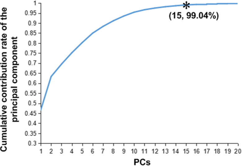
The cumulative contribution rate of the principal components for selecting the number of variables
In this study, 4/5 of the total samples were selected as the training set and 1/5 were selected as the test set based on the Kennard-Stone algorithm (Emerson 2015; Huang et al. 2019), and two different models (i.e., support vector machine (SVM) and random forest (RF) models) were established to classify the kernel type. The particle swarm optimization (PSO, Venter and Sobieszczanski-Sobieski 2003) algorithm was used to select the intercept (c) and the degree of the polynomial (g) of the polynomial kernel for the SVM. The optimal values of c and g for this study were 67.3483 and 0.01, respectively. A comparison of the classification results using the two models is shown in Table 3. In this study, the SVM model was better than the RF model with an 86.11% classification accuracy for the test set.
Table 3.
Comparison results of the different model for kernel type classification (%)
| Model | Dent type | Flint type | Semi-dent type | Average | Average 10-fold cross-validation accuracy | ||||
|---|---|---|---|---|---|---|---|---|---|
| Train accuracy | Test accuracy | Train accuracy | Test accuracy | Train accuracy | Test accuracy | Train accuracy | Test accuracy | ||
| SVM | 85.03 | 78.57 | 90.24 | 86.67 | 87.77 | 89.86 | 88.44 | 86.11 | 78.17 |
| RF | 100 | 71.43 | 100 | 80.00 | 100 | 92.75 | 100 | 82.41 | 76.87 |
Heat mapping of all the extracted maize and kernel traits
In this study, a correlation analysis between the 32 color features, texture features, and morphological features of maize ears, and maize kernels was carried out. The correlations between all the studied feature pairs are presented in Fig. 12. A darker blue on the color scale represents a positive correlation, and a darker red represents a negative correlation.
Fig. 12.

Heat map analysis of the color features, texture features, and morphological features
In this study, under a P value of 0.01, the total kernel number (TKN) was positively correlated with the ear length without the ear barren tip (ELWEBT) (r = 0.76), the ear length (EL) (r = 0.66), the kernel number per row (KNPR) (r = 0.85), the ear area (EA) (r = 0.70), and the ear row number (ERN) (r = 0.54), and was negatively correlated with the kernel thickness (KT) (r = − 0.45), implying that a longer ear with more kernels per row and smaller kernel thickness could yield more kernels. The ear length (EL) was positively correlated with the ELWEBT (r = 0.92), the KNPR (r = 0.78), the EA (r = 0.89), the EP (r = 0.79), and the TKN (r = 0.66), implying that longer ears could yield more kernels per row, larger area, larger perimeter, and more kernels total. The ear length without the ear barren tip (ELWEBT) had a stronger correlation with the KNPR (r = 0.88) and the TKN (0.75) than the ear length, implying that the ELWEBT would strongly affect these traits. The kernel thickness (KT) was negatively correlated with the KNPR (r = − 0.54) and the TKN (r = − 0.45), implying that smaller kernel thickness could result in more kernels per row and more kernels total.
Discussion
A high-throughput maize ear traits scorer (METS) was developed, by which 3 ears can be measured at one time. The time cost of image acquisition was approximately 2 s, and the time cost of image processing for 3 ears was approximately 8–10 s. In total, 34 ear features, namely, 9 color features, 6 texture features, and 19 morphological features of one ear, were extracted. We used 32 of these features to classify the kernel type. In the future, we will establish a kernel type classification model based on deep learning, which needs a robust training set. With a portable power source, the METS could also be used to obtain maize ear traits in the field.
We also compared the measurement accuracy of the METS with that of a commercial maize ear scorer (YTS-MET, Wuhan GreenPheno Science and Technology Co., Ltd., China). We randomly selected 112 maize ear images acquired with YTS-MET to calculate the maize ear length and width. Then, the 112 images of maize ears were also processed using Maize Ear Traits Scorer V 1.0. The correlation coefficients of the ear length and ear diameter between the YTS-MET and METS were 0.86 and 0.94, respectively (Fig. 13). We demonstrated that the image analysis pipeline (Maize Ear Traits Scorer V 1.0) could be extended to other independent maize ear phenotyping platforms.
Fig. 13.

The comparison of the measurement results from this study versus those from a commercial maize ear scorer. a Scatter plots of the measurements with the commercial maize ear scorer versus the measurements of the ear length from the developed maize ear scorer; b scatter plots of the measurements with the commercial maize ear scorer versus the measurements of the ear diameter from the developed maize ear scorer
Conclusion
In this study, we developed a high-throughput maize ear traits scorer (METS) to obtain 9 color features, 6 texture features, and 19 morphological features of maize ears. We evaluated the measurement accuracy and demonstrated the adaptability of the system to different varieties of maize ears. Compared with traditional phenotyping methods of maize ear traits, METS provides an automated, high-throughput, and low-cost (~ 5000 dollars) method for measuring maize ear traits.
Materials availability
The source code and data for this study can be accessed via http://plantphenomics.hzau.edu.cn/download_checkiflogin_en.action.
Supplemental information
(PARTIAL 21068 kb)
(XLS 743 kb)
(DOCX 16 kb)
(RAR 460 kb)
Author contributions
Liang X. processed the images, analyzed the data, and wrote the paper. Ye J. designed the hardware of the system and performed parts of the experiments. Li X. conceived the experiment. Tang Z. analyzed parts of the data. Zhang X., Li W., and Yan J. provided the materials. Yang W. supervised this project and revised the paper.
Funding
This work was supported by the grant from the National Key Research and Development Program (2020YFD1000904-1-3), the National Natural Science Foundation of China (31770397), and the Fundamental Research Funds for the Central Universities (2662020GXPY010, 2662020ZKPY017).
Data availability
The source code and data for this study can be accessed via http://plantphenomics.hzau.edu.cn/download_checkiflogin_en.action.
Declarations
Consent for publication
Consent for publication was obtained from all authors.
Competing interest
The authors declare no competing interest.
Footnotes
Publisher’s note
Springer Nature remains neutral with regard to jurisdictional claims in published maps and institutional affiliations.
Xiuying Liang and Junli Ye contributed equally to this work.
References
- Byun H, Lee SW. Applications of support vector machines for pattern recognition: a survey. Lect Notes Comput Sci. 2002;2388:213–236. doi: 10.1007/3-540-45665-1_17. [DOI] [Google Scholar]
- Chen Y, Xiao C, Chen X, Li Q, Zhang J, Chen F, Yuan L, Mi G. Characterization of the plant traits contributed to high grain yield and high grain nitrogen concentration in maize. Field Crop Res. 2014;159:1–9. doi: 10.1016/j.fcr.2014.01.002. [DOI] [Google Scholar]
- Duan L, Yang W, Huang C, Liu Q. A novel machine-vision-based facility for the automatic evaluation of yield-related traits in rice. Plant Methods. 2011;7:44. doi: 10.1186/1746-4811-7-44. [DOI] [PMC free article] [PubMed] [Google Scholar]
- Dubey BP, Bhagwat SG, Shouche SP, Sainis JK. Potential of artificial neural networks in varietal identification using morphometry of wheat grains. Bios Engin. 2006;95:61–67. doi: 10.1016/j.biosystemseng.2006.06.001. [DOI] [Google Scholar]
- Emerson RW. Convenience sampling, random sampling, and snowball sampling: how does sampling affect the validity of research? J Visual Impair Blind. 2015;109(2):164. doi: 10.1177/0145482X1510900215. [DOI] [Google Scholar]
- Hu W, Zhang C, Jiang Y, Huang C, Liu Q, Xiong L, Yang W, Chen F. Nondestructive 3D image analysis pipeline to extract rice grain traits using X-ray computed tomography. Plant Phenom. 2020;12:3414926. doi: 10.34133/2020/3414926. [DOI] [PMC free article] [PubMed] [Google Scholar]
- Huang H, Zhang DJ, Zhan SY, Shen Y, Wang HZ, Song H, Xu J, He Y. Research on sample division and modeling method of spectrum detection of moisture content in dehydrated scallops. Spectrosc Spectr Anal. 2019;39(1):185–192. doi: 10.3964/j.issn.1000-0593(2019)01-0185-08. [DOI] [Google Scholar]
- Igathinathane C, Pordesimo LO, Batchelor WD. Major orthogonal dimensions measurement offood grains by machine vision using ImageJ. Food Res Int. 2009;42:76–84. doi: 10.1016/j.foodres.2008.08.013. [DOI] [Google Scholar]
- Li L, Zhang Q, Huang D. A review of imaging techniques for plant phenotyping. Sensors. 2014;14:20078–20111. doi: 10.3390/s141120078. [DOI] [PMC free article] [PubMed] [Google Scholar]
- Liang X, Wang K, Huang C, Zhang X, Yan J, Yang W. A high-throughput maize kernel traits scorer based on line-scan imaging. Measurement. 2016;90:453–460. doi: 10.1016/j.measurement.2016.05.015. [DOI] [Google Scholar]
- Liu DY, Zhang W, Liu YM, Chen XP, Zou CQ. Soil application of zinc fertilizer increases maize yield by enhancing the kernel number and kernel weight of inferior grains. Front Plant Sci. 2020;11:188. doi: 10.3389/fpls.2020.00188. [DOI] [PMC free article] [PubMed] [Google Scholar]
- Ma Q, Jiang J, Zhu D, Li S, Mei S. Rapid measurement for 3D geometric features of maize ear based on image processing. Transac Chin Soc Agricult Eng. 2012;28(supp.2):208–212. doi: 10.3969/j.issn.1002-6819.2012.z2.036. [DOI] [Google Scholar]
- Mebatsion HK, Paliwal J, Jayas DS. Automatic classification of non-touching cereal grains in digital images using limited morphological and color features. Comput Electron Agric. 2013;90(1):99–105. doi: 10.1016/j.compag.2012.09.007. [DOI] [Google Scholar]
- Panigrahi S, Misra MK, Willson S. Evaluations of fractal geometry and invariant moments for shape classification of corn germplasm. Comput Electron Agric. 1998;20(1):1–20. doi: 10.1016/S0168-1699(98)00004-0. [DOI] [Google Scholar]
- Rahman MA, Hossain MF, Hossain M, Ahmmed R. Employing PCA and t-statistical approach for feature extraction and classification of emotion from multichannel EEG signal. Egypt Inform J. 2020;21:23–35. doi: 10.1016/j.eij.2019.10.002. [DOI] [Google Scholar]
- Tanabata T, Shibaya T, Hori K, Ebana K, Yano M. SmartGrain: high-throughput phenotyping software for measuring seed shape through image analysis. Plant Physiol. 2012;160:1871–1880. doi: 10.1104/pp.112.205120. [DOI] [PMC free article] [PubMed] [Google Scholar]
- Venter G, Sobieszczanski-Sobieski J. Particle swarm optimization. AIAA J. 2003;41(8):1583–1589. doi: 10.2514/2.2111. [DOI] [Google Scholar]
- Wang H, Sun Y, Zhang T, Zhang G, Li Y, Liu T. Appearance quality grading for fresh corn ear using computer vision. Transac Chin Soc Agricult Machin. 2010;41(8):156–159,165. doi: 10.3969/j.issn.1000-1298.2010.08.032. [DOI] [Google Scholar]
- Wang C, Guo X, Wu S, Du J. Investigate maize ear traits using machine vision with panoramic photograyphy. Transac Chin Soc Agricult Eng. 2013;29(24):155–162. doi: 10.3969/j.issn.1002-6819.2013.24.021. [DOI] [Google Scholar]
- Wu G, Miller ND, Leon N, Kaeppler SM, Spalding EP. Predicting Zea mays flowering time, yield, and kernel dimensions by analyzing aerial images. Front Plant Sci. 2020;10:1251. doi: 10.3389/fpls.2019.01251. [DOI] [PMC free article] [PubMed] [Google Scholar]
- Yang J, Zhang H, Zhao Y, Song X, Wang X. Quantitative study on the relationships between grain yield and ear 3-D geometry in maize. Sci Agric Sin. 2010;43(21):4367–4374. doi: 10.1097/MOP.0b013e3283423f35. [DOI] [Google Scholar]
- Zhao C, Han Z, Yang J, Li N, Liang G. Study on application of image process in ear traits for DUS testing in maize. Sci Agric Sin. 2009;42(11):4100–4105. doi: 10.3864/j.issn.0578-1752.2009.11.043. [DOI] [Google Scholar]
Associated Data
This section collects any data citations, data availability statements, or supplementary materials included in this article.
Data Availability Statement
The source code and data for this study can be accessed via http://plantphenomics.hzau.edu.cn/download_checkiflogin_en.action.