APCI: An R and Stata Package for Visualizing and Analyzing Age-Period-Cohort Data

Abstract

Social scientists have frequently attempted to assess the relative contribution of age, period, and cohort variables to the overall trend in an outcome. We develop an R package APCI (and Stata command apci) to implement the age-period-cohort-interaction (APC-I) model for estimating and testing age, period, and cohort patterns in various types of outcomes for pooled cross-sectional data and multi-cohort panel data. Package APCI also provides a set of functions for visualizing the data and modeling results. We demonstrate the usage of package APCI with empirical data from the Current Population Survey. We show that package APCI provides useful visualization and analytical tools for understanding age, period, and cohort trends in various types of outcomes.

1. Introduction

Researchers across disciplines have long been interested in distinguishing the relative contribution of three time-related variables — namely, age (i.e., how old a person is at the time of data collection), time periods (e.g., the Great Recession 2007–2009 and the COVID-19 pandemic beginning in December 2019), and cohort membership (e.g., the baby boom cohort born in 1945–1964 and the Millennials born in 1981–1996) — to the overall trends in various outcomes (e.g., labor force participation, attitudes, and cognitive functioning) (Alwin and McCammon, 2003; Clogg, 1982; Pescosolido et al., 2021). Decomposing the overall trends into age, period, and cohort variations provides insight into the ways in which biological and social factors affect these outcomes (Hobcraft et al., 1982; Heckman and Robb, 1985; Fosse and Winship, 2019).

To quantify the relative contribution of age, period, and cohort, Luo and Hodges (2020a) have recently developed a model called the age-period-cohort-interaction (APC-I) model. The APC-I is qualitatively different from other age-period-cohort (APC) models in that it characterizes cohort effects as a structure of the age-by-period interaction terms to acknowledge the interdependence of age, period, and cohort effects, whereas prior methods attempt to recover the independent and additive effects of the three variables. The APC-I model has been used to understand the unique contribution of cohort membership in various outcomes including crime involvement, substance use, and cultural taste (Lu and Luo, 2020; Verdery et al., 2020; Ma, 2020). However, the authors of the APC-I model focused on the conceptual motivation of the method and offered relatively few technical details for implementing the method. Estimating and testing cohort effects in the APC-I model may be be challenging for interested readers.

We developed an R package APCI (Xu and Luo, 2021) and a Stata command apci for implementing the APC-I model in empirical research using pooled cross-sectional data (e.g., the General Social Survey and the Current Population Survey) and importantly, extend the APC-I method for analyzing multi-cohort longitudinal or panel data (e.g., data from the Health and Retirement Study (HRS) and the National Longitudinal Study of Youth (NLSY)). The purpose of this paper is three folded. First, we describe the R functions in the APCI package and Stata command to estimate and test age, period, and cohort effects in the APC-I model. The core function can be used for analyzing pooled cross-sectional data and multi-cohort longitudinal data. Second, we introduce a set of visualization tools to help researchers motivate an APC analysis and interpret age, period, and cohort effects from the APC-I model. Third, we clarify several important issues about characterizing cohort effects as a set of age-by-period interaction terms. We pay particular attention to the implications of coding schemes and how to interpret the between-cohort average deviations and within-cohort life-course variations.

This paper is organized as follows. Following a description of traditional APC models and the identification problem, we introduce the APC-I model and the estimation and testing procedures. We explain how and why the age-by-period interaction terms can be used to characterize cohort effects with particular attention to the implications of coding schemes for estimating and testing interactions. Next, we describe the visualization tools and functions in the R package APCI. We then demonstrate how to use the package with the empirical example of men’s and women’s labor force participation from 1990 to 2018 in the United States using data from the Current Population Survey (CPS, Flood et al., 2021).

2. Methodology: the APC-I model

The APC identification problem

To formally estimate and infer the independent age, period, and cohort effects, Mason et al. (1973) specified an analysis of variance (ANOVA) model that they labeled the age-period-cohort (APC) accounting model:

$$g\left(E\left({Ƴ}_{ij}\right)\right)=\mu +{\alpha }_i+{\beta }_j+{\gamma }_k$$ (1)

for age groups i = 1, 2, …, A, periods j = 1, 2, …, P, and cohorts k = 1, 2, …, (A + P − 1), where $\sum _{i=1}^A{\alpha }_i=\sum _{j=1}^P{\beta }_j=\sum _{k=1}^{A+P-1}{\gamma }_k=0$. E(Ƴ_ij) denotes the expected value of the outcome Ƴ for the ith age group in the jth time period; g is the “link function”; α_i denotes the mean difference from the global mean μ associated with the ith age category; β_j denotes the mean difference from μ associated with the jth period; γ_k denotes the mean difference from μ associated with membership in the kth cohort.

Unfortunately, the APC accounting model (1) is not identified even when a coding scheme (e.g., dummy coding where one group is set as the reference group or effect coding where the sum of the coefficients for each effect is set to 0) is applied. This is because age, period, and cohort are exactly linearly related (see Fienberg and Mason, 1979; Fosse and Winship, 2019; Luo et al., 2016, for detailed discussions). As a result, the design matrix of model (1) has rank one less than full, so an infinite number of solutions (i.e., estimates) for the parameters fit the data equally well. That is, the data cannot distinguish different estimation results, so an additional constraint — in addition to the usual reference group or sum-to-zero constraint — must be imposed in order to choose one set of estimates. Moreover, interpreting the results is difficult because the standard interpretation of regression coefficients — that is, the conditional effect of one variable after accounting for other covariates — cannot apply due to the lack of variation in the third variable (e.g., cohort) after considering the other two (e.g., age and period).

The theoretical root of the identification problem in traditional APC models is the problematic assumption that age, period, and cohort effects operate independently of each other. It implies that the identification challenge is inherent in any APC model that attempts to separate independent and additive effects of age, period, and cohort and thus cannot be solved by changing the model setup (e.g., using random effects for period and cohort as in Yang and Land, 2006; see Luo and Hodges, 2020b, for a critique) or by variable manipulation (e.g., using unequal interval widths for age, period, and cohort groups as in Robertson and Boyle, 1986; Sarma et al., 2012; see Luo et al., 2016, for a detailed discussion). The identification problem is well recognized, and its consequences have been discussed extensively (Fienberg and Mason, 1985; Fosse and Winship, 2019; Kupper et al., 1983, 1985; Luo et al., 2016; Luo and Hodges, 2020b; te Grotenhuis et al., 2016; O’Brien, 2020; Morgan and Lee, 2021; Luo, 2013). In essence, internal information derived from the data cannot help because the problem is circular: researchers do the analysis to learn precisely the kind of information needed to justify any such constraint.

The APC-I model

Luo and Hodges (2020a) proposed a new APC model called the age-period-cohort-interaction (APC-I) model. The APC-I model is qualitatively different from all estimators developed under the traditional framework in that it explicitly specifies cohort effects as a structure of the age-by-period interactions. A life-course dynamics hypothesis that concerns about whether and how cohort effects may change as cohorts age thus corresponds to a specific structure of the age-by-period interactions. This specification is motivated by the theoretical account that “The minimal basis for expecting interdependence between inter-cohort differentiation and social change is that change has variant import for persons of unlike age” (Ryder, 1965). That is, a basic notion on which cohort analysis rests is that “transformations of the social world modify people of different ages in different ways.” (Ryder, 1965)

The APC-I model is fully identified in the sense that it does not require additional constraints other than a regular coding scheme. It is also flexible enough to test various hypotheses about life-course changes within cohorts as cohort members age. We first describe the model specification and estimation and testing techniques. The next section demonstrates the procedure using empirical examples.

The general form of the APC-I model can be written as:

$$g\left(E\left({Ƴ}_{ij}\right)\right)=\mu +{\alpha }_i+{\beta }_j+\alpha {\beta }_{ij(k)}$$ (2)

where g, Ƴ_ij, μ, α_i and β_j are defined as in model (1) and αβ_ij(k) denotes the interaction of the ith age group and jth period group, corresponding to the effect of the kth cohort. Note that except for the oldest and youngest cohorts, the effect of one cohort includes multiple age-by-period interaction terms αβ_ij(k) that lie on the same diagonal in a table with ages in rows and periods in columns.

Model (2) differs from model (1) in the way that cohort effects are modeled. In model (2), cohort effects are considered as a specific form of the age-by-period interaction. In statistics, the interaction between two variables describes the differential effects of one variable depending on the level of the other (Scheffé, 1999). In APC research, this means that if part of the overall pattern of interest can be attributed to cohort differences, significant age-by-period interactions should be present. When cohort membership is not associated with the outcome — that is, when the effects of historical or social shifts (period effects) are uniform across age groups — then age-by-period interactions should not be present.

Luo and Hodges (2020a) described a procedure for investigating age and period main effects and inter-cohort deviations and intra-cohort dynamics. They recommended beginning with a deviance test about whether the effects of time periods vary among age groups, which is called “a global F test”. A non-significant global F statistic indicates that there are few age-by-period interaction effects and thus little cohort variation. If the model suggests significant age-by-period interaction effects, one may proceed to examine inter- and intra-cohort differences¹. Inter-cohort average deviations are quantified based on the arithmetic mean of the age-by-period interaction terms contained in each cohort and a t test can be used to examine the average of that cohort-specific deviation. To investigate intra-cohort dynamics over the life course (e.g., the cumulative (dis)advantage hypothesis in Dannefer, 1987; Ferraro and Morton, 2018; Chauvel et al., 2016; O’Brien, 2020), one may use a t-test of the linear orthogonal polynomial contrast in each cohort’s age-by-period interaction effects. This intra-cohort life-course dynamics test is helpful for investigating whether the average (dis)advantages of the members of that cohort accumulate, remain stable, or diminish as they age.

The APC-I model has three advantages. First, it is identified in that it does not require additional constraints other than the usual coding scheme. That is, it avoids the identification problem of the APC accounting model based on the theoretical account of cohort effects and allows inclusion of other important predictors such as education, sex, and employment status. Second, the interpretation of the coefficient estimates of the APC-I model is meaningful and straightforward. This is because the APC-I model recognizes the dependence of age, period, and cohort so the dilemma that analysts face using traditional APC models does not apply. Third, the APC-I model permits investigating life-course dynamics as a cohort ages, whereas extant methods usually assume that cohort effects do not change.

It is important to note that the APC-I model is never intended to “solve” the identification problem in traditional APC accounting models because it is a false problem to begin with. Given the near monopoly of the accounting model, it may be challenging not to see the APC-I method through the lens of the traditional APC accounting framework. For example, because the APC-I model quantifies cohort effects as a structure of the age-by-period interactions, some readers may take it to mean that the APC-I model cannot estimate “linear cohort main effects”. However, the APC-I method, by design, does not intend to estimate any kind of “linear cohort main effects” precisely because the traditional model’s assumption that there is a linear cohort effect that is additive or independent of age and period effects lacks theoretical grounding and is thus arbitrary and questionable. Please see Luo and Hodges (2020a) for a more thorough discussion about the theoretical motivation of the APC-I model.

Because the APC-I mode is relatively new, below we make additional remarks about interaction effects and coding schemes to help readers better understand and use the model.

Interaction effects

In some cases, interaction terms may be difficult to interpret besides suggesting that the effect of one variable may depend on the values of the other. However, as explained by Luo and Hodges (2020a), the age-by-period interaction terms correspond to the conceptual definition of cohort effects and thus can be modeled and interpreted in a meaningful way. Specifically, cohort effects are expected when the influence of social events and changes differ by age groups. This conceptualization of cohort effects implies that the age-by-period interactions, which represent the differential effects of time periods depending on age, can be used to measure cohort effects.

Technically, because of the linear dependency among age, period, and cohort, the effects of the third variable can be expressed as the interaction between the other two variables. The APC-I model considers age and period as main effects and cohort their interactions, which may give the impression that it privileges age and period effects and “discriminates” against cohort effects. The theoretical motivation for this choice is that it is often desirable to estimate a general age pattern that individuals follow as they get older. Period main effects are used to represent the kind of impacts of social environment that everyone in the society is exposed to. The decision to quantify cohort effects as a specific form of age-by-period interaction is informed by the demographic literature on how cohort effects are conceptualized in relation to age and period effects. Empirically, as the analysis of women’s labor force participation in section Examples will illustrate, the size of the cohort effects, characterized as the age-by-period interactions, is not necessarily smaller—in fact may be larger—than some of the main effects.

Coding scheme and contrast

For the unidentified APC accounting model, some estimation methods including the intrinsic estimator yield effect estimates that are dependent on the choice of coding schemes in that estimates under different coding schemes are not equivalent (see Luo et al., 2016; te Grotenhuis et al., 2016, for a more detailed discussion). The APC-I model does not have a rank deficiency problem in the sense that it does not require more constraints than a usual ANOVA model with main effects and their interactions. For any identified model including the APC-I model, the estimates are equivalent; that is, the estimated cell means are the same for all coding schemes.

Although this equivalence holds for both main effects and interaction estimates in the APC-I model, it is less obvious for interaction terms because the interpretation of the specific parameter estimates do change with coding schemes. To illustrate, consider an example of applying the APC-I model to health data with three age categories and three periods, shown in table 1 below. Under dummy coding—for example, the youngest age group 20–24 and the beginning survey period of 2000 are set to zero or omitted as the referent—the interaction for ages 25–29 and period 2005 in cell Ƴ represents the difference in a health outcome between periods 2000 and 2005 for age 25–29 or equivalently, health difference between ages 25–29 and 20–24 for the period 2005. That is, interactions under dummy coding represents a directional difference from a particular reference group.

Table 1:

Hypothetical data with three age categories and three periods illustrating a shift in meaning and interpretation of interaction terms under different coding schemes. The interaction terms under different types of coding in cell Ƴ necessarily have different numerical values because of different reference groups. For example, the interaction term in cell Ƴ under dummy coding represents a directional difference from a particular reference group (e.g., age 20–24 in year 2000). Under effect coding, the same interaction term in cell Ƴ represents the deviation in the outcome from the age main effect plus period main effect for the group of individuals who were age 25–29 and surveyed in period 2005. Such different numeric values do not arise from an identification problem but rather from a shift in what these quantities represent.

		Period
		2000	2005	2010
Age	20–24
	25–29		Ƴ
	30–34

By contrast, under effect coding (i.e., sum-to-zero coding), the same interaction term in cell Ƴ represents the deviation in the health outcome from the age main effect plus period main effect for the group of individuals who were age 25–29 and surveyed in period 2005.

The estimated interaction terms under these two types of coding in cell Ƴ thus necessarily have different numerical values. However, this difference does not arise from an identification problem but rather from a shift in what these quantities represent. That is, the two interaction terms can be transformed to be equivalent so that the means in Ƴ after considering age and period main effects are the same under the two coding schemes.

We recommend using effect or sum-to-zero coding for estimating the APC-I model for the following reasons: when characterizing cohort effects as a set of age-by-period interactions, we are less concerned about any direction of the interactions; that is, we are not particularly interested in the difference between two cohorts at a particular age or time period. Rather, we focus on particular structures of these interactions that may represent theoretically interesting patterns during a cohort’s life span. Effect coding is helpful because they all have the same referent group — the next lower level in the hierarchy of main effects and interactions. That is, we choose effect coding for the purpose of easy interpretation. This is also consistent with the recommendation of coding schemes in the presence of interactions (Aiken et al., 1991; Jaccard and Turrisi, 2003).

3. The R package APCI

Package installation

The R package APCI² can be installed and loaded using the following R code³:

# install R package APCI
> install.packages(“APCI”)
# load R package APCI to the current working environment
> library(APCI)

The main routines to implement the APC-I model using package APCI are apci.plot.raw, apci, apci.plot (or apci.plot.hexagram, apci.plot.heatmap). A summary of these functions and input arguments used in the routines are described below.

Functions in R package APCI

The R package APCI contains the following functions for estimating the APC-I model and visualizing the data and the model results:

• apci: to estimate the age, period, and cohort effects using the APC-I model.

• temp_model: an internal function that estimates a generalized linear model.

• tests: to conduct the global F test.

• maineffect: an internal function to extract age and period main effects.

• cohortdeviation: an internal function to extract between-cohort average deviations and within-cohort life-course dynamics.

• ageperiod_group: to return a cohort index based on how age and period are grouped.

• apci.plot.raw: to visualize the mean values of the outcome across age and period groups, respectively.

• apci.plot.hexagram: to visualize the estimated cohort effects in a hexagram style.

• apci.plot.heatmap: to visualize the estimated cohort effects in a heatmap style.

• apci.plot: to visualize the estimated age, period, and cohorts in conventional figures.

A summary of input arguments required in these functions will be given one by one ⁴ in the next section. Package APCI also contains three empirical datasets women9017, cpsmen, cpswomen, and one simulated dataset simulation. Dataset women9017 was used and described in Luo and Hodges (2020a). Applications of the APC-I model to the other two empirical datasets are given in section Examples.

Function apci

Function apci is the core function in the R package APCI. It fits an APC-I model with or without covariates and returns a list of results including coefficients and standard error estimates for age main effects, period main effects, inter-cohort average deviations, and intra-cohort life-course trends, and covariate coefficients if any. Both pooled cross-sectional data and multi-cohort longitudinal/panel data are supported. Specifically, function apci is used as

apci(data, outcome, age, period, cohort, weight, covariate, family,
        dev.test=TRUE, print, gee, id, corstr,…)

and takes the following arguments:

• data: a data frame containing an outcome variable, age group indicators, period group indicators, and covariates to be used in the model. If a variable is not found in data, there will be an error message reminding users to check the input data again. Supported data structures include pooled cross-sectional data and multi-cohort longitudinal/panel data.

• outcome: an object of class character containing the name of the outcome variable. The outcome variable can be a continuous, categorical, or count variable.

• age: an object of class character indicating the age group index taking on the number of distinct values in the data (e.g., six age groups: 20–24, 25–29, 30–34, 35–39, 40–44, and 45–49). The vector should be a factor (or “category”, or “enumerated type”).

• period: an object of class character indicating the time period index in the data.

• cohort: an optional object of class character indicating cohort membership index in the data. The cohort index can be generated from the age group index and time period index in the data because of the exact linear relationship among these three time-related indices.

• weight: an optional vector of sample weights to be used in the model fitting process. If non-NULL, user-supplied weights will be used in the first step to estimate the model. Observations with negative weights will be dropped in modeling.

• covariates: an optional vector of characters containing the names of user-specified covariate(s) to be used in the model. If the variables are not found in data, there will be an error message reminding the users to check the data again.

• dev.test: logical, specifying if the global F test (step 1) should be implemented before fitting the APC-I model. If TRUE, apci will first run the global F test and report the test results; otherwise, apci will skip this step and return NULL. The default setting is TRUE. However, users should be aware that the algorithm will not automatically stop even if there is no significant age-by-period interactions based on the global F test.⁵

• family: a character string specifying the link function to be used in the model. The value can be “binomial”, “multinomial”, or “gaussian”. See R function glm for more details about link functions.

• print: logical, specifying if the intermediate results should be displayed in the console when fitting the model. The default setting is TRUE to display the results of each procedure.

• gee: logical, indicating if the data is cross-sectional data or longitudinal/panel data. If TRUE, the generalized estimating equation will be used to correct the standard error estimates. The default is FALSE, indicating that the data are cross-sectional.

• id: a character vector specifying the cluster index in longitudinal data. It is required when gee is TRUE. The length of the vector should be the same as the number of observations.

• corstr: a character string specifying a possible correlation structure in the error terms when gee is TRUE. The following are allowed: independence, fixed, stat_M_dep, non_stat_M_dep, exchangeable, AR-M and unstructured. The default value is exchangeable.

• unequal_interval: logical, indicating if age and period groups are of the same interval width. The default is set as TRUE.

• age_range,period_range: numeric vectors indicating the actual age or period range (e.g., 10 to 59 years old or from 2000 to 2019).

• age_interval,period_interval,age_group,period_group: numeric values or character vectors indicating how age and period are grouped. age_interval and period_interval indicate the width of age and period intervals, respectively. age_group and period_group are character vectors listing possible age and period groups. There are two ways to define age and period groups with unequal intervals: 1) defining age_interval and period_interval, or 2) defining age_group and period_group. Users must define age and period groups using one of the two options when unequal_interval is TRUE.

• …: further optional arguments to be passed to the model.

As mentioned in section Coding scheme and contrast, we use effect coding to estimate the APC-I model. The age and period arguments in function apci accept categorical variables. Different from the common approach of dummy coding or simple coding, where an effect is defined as the difference of each group from the reference group, function apci uses effect coding (i.e., the sum-to-zero coding, deviation coding, or the ANOVA coding) as the default coding. Under this coding scheme, the effect of the omitted category equals the negative sum of the effects of all other categories. Computation wise, the effect coefficient of the omitted category is redundant because of the coding scheme. However, for the purpose of quantifying cohort effects as deviations from the main effects of age and period, it is useful to compute estimates for all age-by-period cross-classifications and their standard errors. For data with A age groups and P periods, therefore, function apci returns A and P number of main effect estimates and A * P number of interaction estimates along with their standard error estimates. For the main effects of age or period, the estimate can be interpreted as the deviation associated with each age or period group from the global mean. The age-by-period interactions represent the deviation from the expectation determined by the corresponding age and period main effects.

Also note that when age and period groups have unequal interval widths in an age-period classification table, the age-by-period interactions contained in a cohort no longer lie on the same diagonals. Because cohort effects are conceptualized and estimated as a structure of the age-by-period interactions in the APC-I model, it is technically possible to use the argument unequal_interval in package APCI to extract interaction coefficient estimates that lie on different diagonals. However, unequal age and period group intervals may complicate the issue of cohort overlapping noted by Kupper et al. (1985). For this reason, we do not recommend using unequal interval widths for age and period groups if possible.

After fitting the APC-I model, function apci will store the following components as a list for further usage:

• model: a summary of the fitted generalized linear regression model.⁶ It displays the standard regression output including coefficient and standard errors estimates.

• dev_global: the global F test results. It examines if the interaction terms are significant in a generalized linear regression model that contains age and period main effects and their interactions.

• intercept: the overall intercept (μ in equation 2).

• age_effect: a vector containing the estimated effect for each age group.

• period_effect: a vector containing the estimated effect for each time period.

• cohort_average: a vector containing the inter-cohort average deviations for comparing differences between cohorts.

• cohort_slope: a vector containing intra-cohort life-course trends.

Function tests

As mentioned earlier, the first step of implementing the APC-I model is to conduct a global F test of the age-by-period interactions. This step is a routine in function apci, but the procedure does not stop even if there is no statistically significant deviation from the age main effect and period main effect. Therefore, we recommend separately conducting the global F test. In R package APCI, the function tests can be used for this purpose. It can be used as follows:

tests(model, A, P, C, …)

and takes the following arguments:

• model: a generalized linear regression model generated from the internal function temp_model.⁷

• A, P, C: numbers of age groups, period groups, or cohort groups. If age and period groups are of different widths, the values of will be automatically generated by the function.

Function tests will return a standard F test result including the value of the F test statistic and the associated p-value.

Functions for visualization

In package APCI, we provide four functions to facilitate visualizing the data and model results, namely apci.plot.raw, apci.heatmap, apci.plot.hexagram, and apci.plot, in different stages of a research project. They take similar input arguments. A summary of these arguments is given below.

Function apci.plot.raw is designed to plot the outcome variable aggregated by age or period groups. This function may be used in the stage of data exploration. Functions apci.heatmap and apci.plot.hexagram are designed to plot the age-by-period interactions from the APC-I model. Both functions generate heatmaps, where one axis represents age groups, and the other period groups. The cells in a diagonal represent one cohort. The difference between the two functions is the layout of the heatmap; one is a rectangular graph and the other a hexagram. Function apci.plot can be used to visualize both raw data and model results. It divides the canvas into four (2 × 2) panels. Three of the four panels can be used to visualize the three effect estimates in the APC-I model and the left panel to add notes. For data exploration, users can visualize the mean values of the outcome variable across age, period, and cohort groups on the same canvas. Users can the same functions to visualize the estimated age, period, and cohort effects from the modeling results.

The visualization functions in package APCI include:

apci.plot.raw(data, outcome_var, age, period, …)
apci.plot.heatmap(model, age, period, color_map = NULL, color_scale = NULL,
        quantile = NULL, …)
apci.plot.hexagram(model, age, period, first_age, first_period, interval,
        color_scale = NULL, color_map = NULL, quantile = NULL, …)
apci.plot(model, age, period, outcome_var, type = “model”, quantile = NULL,
        …)

and takes the following arguments:

• model: a list recording the results from function apci.

• outcome_var: an object of class character indicating the name of the outcome variable used in the model. The outcome variable can be a continuous, binary, categorical, or count variable.

• age: a vector indicating the age group. The vector should be converted to a factor (or the terms of “category” and “enumerated type”).

• period: a vector indicating the time period. The vector should be converted to a factor (or “category”, “enumerated type”).

• color_map: a vector representing a color palette to be used in the figure. The default setting is greys if color_map is NULL. Alternatives, for example, can be c(“blue”, “yellow”), “blues”, etc.

• cohort_scale: a vector containing two values to indicate the minimum and maximum values, respectively, of the estimated cohort effects to be displayed. If NULL, the function will use the range from the estimation results.

• quantile: a number valued between 0 and 1, representing the desirable percentiles to be used in visualizing the data or model. If NULL, the original scale of the outcome variable will be used.

4. Examples: Application of the R package APCI to empirical data

We now illustrate how to use package APCI’s visualization and analytical functions. We describe and analyze two empirical datasets to demonstrate how this package may be used to analyze pooled cross-sectional data. We later briefly describe how to fit an APC-I model for multi-cohort longitudinal data.

Cross-sectional data of labor force participation in the United States

Temporal trends in men’s and women’s labor force participation (LFP) in United States have gathered much scholarly attention (see e.g. Connelly, 1992; Farkas, 1977; Hollister and Smith, 2014; Macunovich, 2012; Treas, 1987; Wilkie, 1991). For example, whereas men’s LFP steadily declined in the past decades (Wilkie, 1991), women’s LFP continued to rise until the 1990s and the 2000s. Female LFP has since then reached a plateau and even begun to decline. Researchers have debated about the causes of this leveling off or decline. Some studies attributed the observed trends to period-specific factors such as labor demand (Erceg and Levin, 2014), the economic shocks of the Great Recession (Boushey, 2005; Hoffman, 2009), social welfare and disability insurance (Duggan and Imberman, 2009), and gender role attitudes (Fortin, 2015).

However, the temporal trends in LFP are unlikely due to a pure period process. For example, because individuals may begin to leave the labor force in age 50, a decline in LFP should be expected if the proportion of the population age 50 or older has increased. That is, the recent trends may reflect a change in the age composition of the US population (Aaronson et al., 2014). The cohort succession may also contribute to the trend, a process in which older cohorts with higher or lower LFP rates begin to decease and younger cohorts with lower or higher LFP enter the labor force Lee (2014). At the same time, critical social and demographic changes in education level, fertility, and attitudes about women working outside the home may be more of cohort-specific than period-specific processes because these forces only affect individuals of certain ages (Balleer et al., 2014; Farré and Vella, 2013; Fernández, 2013; Goldin, 2006).

Given that the observed trends in LFP are likely a mix of age, period, and/or cohort patterns, an APC analysis that decomposes the temporal trends into age-, period-, and cohort-related variations is thus helpful for revealing the demographic, social, and economic changes that have underlined the temporal trends in American’s labor force participation. In this following section, we demonstrate how to use the functions in APCI to undertake an APC analysis of men’s and women’s LFP using a cross-sectional dataset.

The Current Population Survey (CPS, Flood et al., 2021) is the primary source of labor force statistics in the United States (Flood et al., 2021). Beginning in the 1960s, the CPS has been collecting data on key demographic, economic, and education topics. We subset the 1990–2019 CPS data by gender, resulting in two datasets, namely cpsmen and cpswomen, to show how to conduct an APC-I analysis of men’s and women’s LFP in the United States using package APCI.

Datasets cpsmen and cpswomen contain a subset of men and women age 20–64 who participated in the 1990 to 2019 CPS. The following code is used to load the data into the working environment:

> data(cpsmen)
> data(cpswomen)

The first five rows of the datasets of cpsmen and cpswomen are:

> head(cpsmen, n = 5)
  asecwt year age labforce educc
 2854.84    3   5        0     1
 1576.54    4   4        1     2
 2340.55    2   6        1     3
  158.44    3   5        0     0
  347.09    6   6        1     3

> head(cpswomen, n = 5)
  asecwt year age labforce educc
 2415.67    2   3        1     1
  663.89    2   5        1     3
 1653.01    6   4        1     2
 1613.31    6   4        0     2
  177.23    4   3        1     2

where labforce indicates the respondent’s labor force participation status (1=in the labor force, 0=not in the labor force). asecwt is the person-level weight that the CPS recommends to be used in individual-level data analyses. year indicates the survey year when respondent was interviewed, grouped into 6 period groups (1=1990–94, 2=1995–99, …, 6=2015–19). age indicates the respondent’s age categories (1=20–24, 2=25–29, …, 9=60–64). educc is a three-level categorical education measure (1=less than high school, 2=high school graduate, 3=college degree or above).

For data exploratory purpose, function apci.plot.raw visualizes the outcome variable in the following way:

> apci.plot.raw(data, outcome_var, age, period)

Figure 1 shows LFP rates by age groups (top panel) and period groups (bottom panel), respectively, for male (left panel) and female CPS respondents (right panel) age 20 to 64 from 1990 to 2019. Figure 1‘s top panel suggests similar age patterns in LFP across time periods. The bottom panel shows distinct period trends depending on age groups. For example, the LFP rates among women in the 55–59 and 60–64 age groups seem to have gone up whereas other age groups show a relatively flat trend. Such distinct period patterns in LFP by age groups suggest potential cohort variations in women’s labor force participation. For men’s LFP, however, the visualization results suggest that a simpler model with age and period main effects may suffice for summarizing their LFP patterns.

Figure 1:

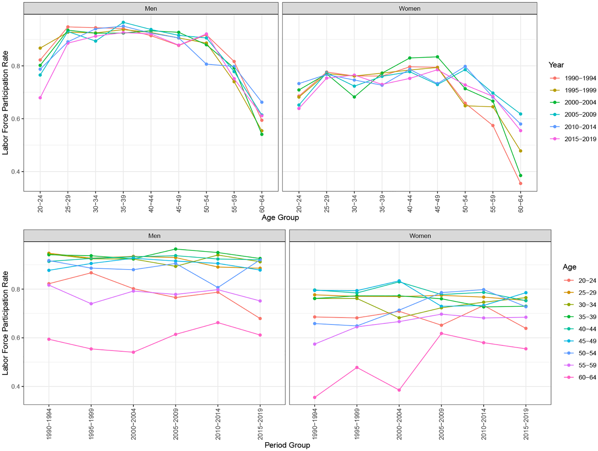
Period-specific age trajectories and age-specific period trends in labor force participation rates for men and women in the United States, the Current Population Survey 1990–2019. Age trajectories are similar across time periods for both men and women (top panel). Period trends differ by age groups, especially among women (bottom panel).

Function apci can be used to fit an APC-I model for pooled cross-sectional data or multi-cohort longitudinal/panel data. In the simplest form of an APC-I model without covariates for pooled cross-sectional data, function apci is called as follows:

> no_cov <- APCI::apci(outcome = “labforce”,
+                      age = “age”,
+                      period = “year”,
+                      weight = “asecwt”,
+                      data = cpswomen,
+                      dev.test = FALSE,
+                      family = “binomial”)

It is often desirable to add covariates in the model, which can be done by calling the covariate argument. For example, suppose one would like to add education levels (“educc”) as a covariate in the model, function apci can be used as:

> with_cov <- APCI::apci(outcome = “labforce”,
+                        age = “age”,
+                        period = “year”,
+                        covariate = c(“educc”),
+                        weight = “asecwt”,
+                        data = cpswomen,
+                        print=F,
+                        dev.test=FALSE,
+                        family = “binomial”)

Below is a summary of the results from an APC-I model that includes education levels as a covariate:

> summary(with_cov)
               Length Class      Mode
model          33     svyglm     list
dev_global      0     -none-     NULL
intercept       4     -none-     character
age_effect     45     -none-     character
period_effect  30     -none-     character
cohort_average  6     data.frame list
cohort_slope    6     data.frame list
int_matrix      5     data.frame list
cohort_index   54     -none-     numeric
data            7     data.frame list

The returned value is a list of objects. model contains the results from a logistic regression model with age and period main effects and the unstructured interactions. dev_global displays the global F test result. A significant F statistic suggests that there may exist cohort effects. intercept is the overall intercept (μ in Equation 2). age_effect gives estimated age main effect. period_effect is the estimated period main effect. cohort_average gives inter-cohort average deviations from age and period main effects. cohort_slope gives intra-cohort life-course linear slopes, which can be used for testing intra-cohort life-course dynamics. int_matrix displays a matrix that contains the estimated coefficients for age-by-period interactions. Note that there are A*P interactions in int_matrix because effect coding is used to compute the A+P-1 interaction estimates based on the (A-1)*(P-1) freely varying interaction parameters. Such interaction estimates are used to generate heatmaps similar to Figure 2. data stores the data fed into apci function. Users may call an object to obtain detailed results. For example, by calling with_cov$cohort_average and with_cov$cohort_slope, users can obtain estimated inter-cohort average deviations and intra-cohort life-course slopes.

Figure 2:

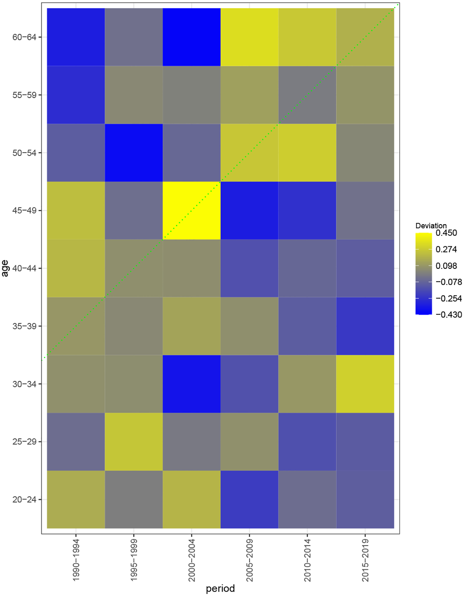
Cohort deviation heatmap showing higher-than-expected labor force participation rates that persist over their life course for the 1955 birth cohort. Each square represents an age-by-period interaction. Yellow squares indicate lower participation rates than the expectation determined by the age and period main effects. Blue squares indicate higher-than-expected rates. Each diagonal that runs from the lower left to the upper right represents one birth cohort. The dotted line indicates a significant average inter-cohort deviation but an insignificant intra-cohort slope in their labor force participation rates for the 1955 cohort.

The output below shows education-adjusted inter-cohort average deviations in women’s LFP from analyzing the cpswomen data using function apci.

> with_cov$cohort_average
   c_avg_group c_avg_est c_avg_se c_avg_t c_avg_p c_avg_sig
1            1    -0.329    0.193  -1.709   0.088
2            2    -0.155    0.142  -1.091   0.275
3            3    -0.162    0.114  -1.422   0.155
4            4     0.047    0.097   0.481   0.631
5            5     0.096    0.085   1.139   0.255
6            6     0.174    0.076   2.288   0.022      *
7            7     0.034    0.074   0.457   0.648
8            8    -0.036    0.074  -0.493   0.622
9            9     0.003    0.073   0.047   0.963
10          10    -0.072    0.081  -0.894   0.371
11          11     0.030    0.085   0.353   0.724
12          12    -0.029    0.102  -0.288   0.774
13          13    -0.080    0.131  -0.609   0.543
14          14    -0.103    0.170  -0.608   0.543

where c_avg_group indicates cohort membership (e.g., cohort 1=the 1930 birth cohort, cohort 2=the 1935 birth cohort,…,cohort 14=the 1995 birth cohort), c_avg_est is inter-cohort average deviation, c_avg_se is the standard error estimate for the average deviation, c_avg_t is the t test statistic for the average deviation, and c_avg_p and c_avg_sig are the p values and alpha levels (*: p < .05, **: p < .01, and ***: p < .001), respectively.

The results from with_cov$cohort_average imply that on average, the LFP rates among cohort 6’s–the 1955 birth cohort – significantly differ from the expected rates based on age and period main effects. Specifically, the 1955 cohort shows a .19 (exp(.174)-1, p < .05) higher participation rate than the expectation based on the age and period main effects.

The output below shows education-adjusted intra-cohort life-course dynamics in women’s LFP from analyzing the cpswomen data using function apci.

> with_cov$cohort_slope
   c_slp_group c_slp_est c_slp_se c_slp_t c_slp_p c_slp_sig
1            1        NA       NA      NA      NA      <NA>
2            2     0.165    0.195   0.849   0.396
3            3    -0.215    0.187  -1.148   0.251
4            4     0.163    0.189   0.866   0.386
5            5     0.093    0.184   0.508   0.611
6            6     0.007    0.169   0.039   0.969
7            7     0.047    0.172   0.277   0.782
8            8    -0.096    0.181  -0.530   0.596
9            9    -0.187    0.173  -1.076   0.282
10          10    -0.106    0.176  -0.602   0.547
11          11    -0.279    0.159  -1.750   0.080
12          12     0.353    0.160   2.207   0.027       *
13          13    -0.047    0.180  -0.262   0.793
14          14        NA       NA      NA      NA      <NA>

where c_slp_group indicates cohort membership (e.g., cohort 1=the 1930 birth cohort, cohort 2=the 1935 birth cohort,…, cohort 14=the 1995 birth cohort), c_slp_est is intra-cohort life-course slopes, c_slp_se is the standard error estimate for the life-course slope, c_slp_t is the t test statistic for the life-course slope, and c_slp_p and c_slp_sig are the p values and alpha levels (*: p < .05, **: p < .01, and ***: p < .001), respectively. NAs are generated for the youngest and oldest cohort because there is only one age-by-period combination observed for the two cohorts and thus intra-cohort life-course dynamics cannot be accessed.

For example, for cohort 12 (the 1985 birth cohort), the estimated intra-cohort slope is 0.353 (p < .05), meaning that this cohort’s LFP is lower than expected when they were young but higher than expected in older ages. Interestingly, for cohort 12 (the 1985 birth cohort), their average cohort deviation is not statistically significant. Such an insignificant inter-cohort average deviation and a significantly negative intra-cohort slope indicate a compensation life-course pattern; that is, this cohort’s lower-than-expected LFP in younger ages seems to be compensated by their higher LFP when they were older.

The intra-cohort life-course dynamics are based on the age-by-period interactions as follows:

# the first six rows of the life-course dynamics
> with_cov$int_matrix
  iaesti  iase   iap iasig cohortindex
1  0.166 0.169 0.327                 9
2 -0.048 0.207 0.818                 8
3  0.068 0.164 0.678                 7
4  0.095 0.172 0.581                 6
5  0.205 0.191 0.283                 5
6  0.227 0.193 0.239                 4
# [there are 48 rows compressed]

where “iaesti” is the age-by-period interaction estimates, “iase” is the standard error estimate for the interaction term, “iap” and “iasig” are the p value and alpha level (*: p < .05, **: p < .01, and ***: p < .001),respectively, and “cohortindex” indicates cohort membership.

The following code can be used to organize the intra-cohort life-course estimates in a matrix form:

> matrix(with_cov$int_matrix, A, P)[A:1,]
# A is the number of age groups and P is the number of period groups.
       period #1 period #2 period #3 period #4 period #5 period #6
age #9 -0.329    -0.038    -0.416*    0.334     0.267     0.182
age #8 -0.272     0.043     0.017     0.125     0.001     0.086
age #7 -0.112    -0.392*   -0.070     0.257     0.278     0.040
age #6  0.227    -0.046     0.443*   -0.333*   -0.258    -0.033
age #5  0.205     0.066     0.061    -0.150    -0.074    -0.107
age #4  0.095     0.044     0.139     0.065    -0.109    -0.234
age #3  0.068     0.059    -0.359*   -0.147     0.096     0.283
age #2 -0.048     0.256    -0.006     0.067    -0.156    -0.113
age #1  0.166     0.009     0.191    -0.216    -0.046    -0.103

Based on the R package ggplot2 (Wickham, 2016), heatmaps can be generated to visualize inter- and intra-cohort patterns and motivate a subsequent formal APC analysis. For example, for dataset whitemen, both inter-cohort average deviations and intra-cohort life-course dynamics may be visualized in a heatmap as follows:

> apci.plot.heatmap(model = with_cov, age = “age”,period = ‘year’,
                  color_map = c(‘blue’,’yellow’))

Figure 2 is a heatmap of the estimated age-by-period interactions, with rows defined by age groups and columns by time periods. Each square represents an age-by-period interaction. Yellow squares indicate lower participation rates than the expectation determined by the age and period main effects. Blue squares indicate higher-than-expected rates. Each diagonal that runs from the lower left to the upper right represents one birth cohort. The dotted line in Figure 2 indicates a significant inter-cohort average deviation but an insignificant intra-cohort slope in their LFP for the 1955 cohort. Cohorts that on average significantly deviate from the expected rates based on age and period main effects are indicated by solid, dashed, or dotted lines. Solid lines indicate significantly (p<.05) positive intra-cohort life-course slopes, dashed lines significantly negative intra-cohort slopes, and dotted lines significant average inter-cohort deviations but insignificant intra-cohort slopes. Users have the options to customize the elements of these figures to suit their research or teaching purposes.

Figure 2 indicates that although some cohorts had LFP rates that differ from the expected rates based on age and period main effects, only the 1955 birth cohort (marked by a dotted line) had, on average, higher-than-expected LFP rates (inter-cohort average deviation = .174, p < .05), and this higher LFP seems to persist over their life course (intra-cohort slope = .007, p = .969). This visualization results are consistent with the results from with_cov$cohort_average and with_cov$cohort_slope.

Users can also use bar plots to visualize inter-cohort average deviations. Function apci.bar can be used as:

> apci.bar(model = with_cov, age = “age”,period = “year”,
            cohort_label = seq(1930,1995,5))

Figure 3 illustrates inter-cohort deviations based on the average of the age-by-period interaction estimates contained in each cohort. The horizontal line at y=0 indicates expectations for all cohort based on the main effects of age and period when they are observed. The bars indicate the estimated average deviation for each cohort from the age and period main effects. Bars above the horizontal line indicate positive average deviations, and bars below the line indicate negative average deviations. The asterisk sign indicates that a cohort’s average deviation is significantly different from the expectation determined by age and period main effects. Figure 3 suggests some cohort variation in women’s LFP using the 1990–2019 CPS data, but only the 1955 birth cohort had significantly higher-than-expected LFP rates.

Figure 3:

Bar plots showing inter-cohort average deviations in women’s labor force participation rates. Only the 1955 birth cohort had a significantly higher-than-expected participation rate. The horizontal line at y=0 indicates expected labor force participation rates for each cohort based on the main effects of age and period when they were observed. The bars indicate the estimated average deviation for each cohort from the age and period main effects. Bars above the horizontal line indicate positive average deviations, and bars below the line indicate negative average deviations. The asterisk sign indicates that a cohort’s average deviation is significantly different from the expectation determined by age and period main effects at the .05 or lower level.

Longitudinal data

For longitudinal data (i.e., panel data, repeated measure data) that include multiple cohorts, users may set the argument gee to TRUE to estimate an APC-I model using the generalized estimating equation (GEE) technique (Liang and Zeger, 1986; Carey et al., 2019). When gee is TRUE, users will also need to specify arguments id and corstr accordingly.

> model_gee <- apci(outcome = “y”,
+                  age = “age”,
+                  period = “period”,
+                  cohort = NULL,
+                  weight = NULL,
+                  covariate = NULL,
+                  data=simulation_gee,
+                  family =“gaussian”,
+                  dev.test = FALSE,
+                  print = TRUE,
+                  gee = TRUE,
+                  id = “id”,
+                  corstr = “exchangeable”)
> summary(model_gee)

The list of output results is similar to that for pooled cross-sectional data, but the standard errors are corrected using the GEE’s sandwich estimator.

5. Use the R package APCI in Stata

We also designed a Stata command apci based on the Stata command rcall (Haghish, 2019) to help implement APC-I models in Stata. The command is used as:

apci depvar [indepvars], outcome(depvar) age(age) period(period) family(“gaussian”) [if] [in] [weight]

Stata users can use the above command to fit APC-I models and obtain all the results as in R. A Stata ado file for installing this command can be downloaded at https://sites.psu.edu/liyingluo/software/.

6. Conclusion and future development

In this article, we introduced an R package APCI and Stata command apci for implementing the age-period-cohort-interaction (APC-I) model developed by Luo and Hodges (2020a). In addition to pooled cross-sectional data analysis, we extended the package to permit multi-cohort longitudinal or panel data analysis. This package also contains a set of visualization tools to help researchers motivate an APC analysis and interpret the results. We clarify the implications of coding schemes for estimating and testing main effects and interaction effects in the APC-I model. We illustrate how to use this package using the empirical examples of labor force participation using the 1990–2019 data from the Current Population Survey.

Luo and Hodges (2020a) described a local F test for testing the variation associated with the multiple age-by-period interactions contained in each cohort. Because the parameterization of the local F test is more intricate than it appears, the R package APCI and the Stata command apci currently do not support such tests as of version 1.0.5 but may be available in later versions.

Moreover, it may be of interest to examine the interaction effects of cohort and other explanatory variables such as education and geographic areas. Because cohort effects are conceptualized and operationalized as a two-way interaction term of age and period effects, an interaction term between cohort and another variable is equivalent to a three-way interaction among age, period, and another variable. Future development may consider creating functions to facilitate summarizing and interpreting the more complex three-way interaction terms in the APC-I model.

Bibliography

- Aaronson S, Cajner T, Fallick B, Galbis-Reig F, Smith C, and Wascher W. Labor Force Participation: Recent Developments and Future Prospects. Brookings Papers on Economic Activity 2014, (2): 197–275, 2014. URL https://www.brookings.edu/bpea-articles/labor-force-participation-recent-developments-and-future-prospects/. [Google Scholar]
- Aiken LS, West SG, and Reno RR. Multiple Regression: Testing and Interpreting Interactions. SAGE, 1991. ISBN 978–0-7619–0712-1. Google-Books-ID: LcWLUyXcmnkC. [Google Scholar]
- Alwin DF and McCammon RJ. Generations, Cohorts, and Social Change. In Mortimer JT and Shanahan MJ, editors, Handbook of the Life Course, Handbooks of Sociology and Social Research, pages 23–49. Springer US, Boston, MA, 2003. ISBN 978–0-306–48247-2. doi: 10.1007/978-0-306-48247-2_2. URL 10.1007/978-0-306-48247-2_2. [DOI] [Google Scholar]
- Balleer A, Gomez-Salvador R, and Turunen J. Labour force participation across Europe: A cohort-based analysis. 46(4):1385–1415, 2014. ISSN 1435–8921. URL https://econpapers.repec.org/article/sprempeco/v_3a46_3ay_3a2014_3ai_3a4_3ap_3a1385-1415.htm. [Google Scholar]
- Boushey H. Are Women Opting Out? Debunking the Myth. Center for Economic and Policy Research (CEPR), pages 2005–36, 2005. [Google Scholar]
- Carey VJ, Lumley TS, Moler C, and Ripley B. gee: Generalized Estimation Equation Solver, 2019. URL https://CRAN.R-project.org/package=gee. R package version 4.13–20.
- Chauvel L, Leist AK, and Ponomarenko V. Testing Persistence of Cohort Effects in the Epidemiology of Suicide: An Age-Period-Cohort Hysteresis Model. PLOS ONE, 11(7):e0158538, July 2016. ISSN 1932–6203. doi: 10.1371/journal.pone.0158538. [DOI] [PMC free article] [PubMed] [Google Scholar]
- Clogg CC. Cohort Analysis of Recent Trends in Labor Force Participation. Demography, 19(4):459–479, Nov. 1982. ISSN 0070–3370, 1533–7790. doi: 10.2307/2061013. URL https://link.springer.com/article/10.2307/2061013. [DOI] [PubMed] [Google Scholar]
- Connelly R. The Effect of Child Care Costs on Married Women’s Labor Force Participation. The Review of Economics and Statistics, 74(1):83–90, 1992. [Google Scholar]
- Dannefer D. Aging as Intracohort Differentiation: Accentuation, the Matthew Effect, and the Life Course. Sociological Forum, 2(2):211–236, 1987. ISSN 0884–8971. URL https://www.jstor.org/stable/684472. Publisher: [Wiley, Springer]. [Google Scholar]
- Duggan M and Imberman SA. Why are the disability rolls skyrocketing? the contribution of population characteristics, economic conditions, and program generosity. In Health at Older Ages, pages 337–380. University of Chicago Press, 2009. [Google Scholar]
- Erceg CJ and Levin AT. Labor Force Participation and Monetary Policy in the Wake of the Great Recession. Journal of Money, Credit and Banking, 46(S2):3–49, 2014. ISSN 1538–4616. doi: 10.1111/jmcb.12151. [DOI] [Google Scholar]
- Farkas G. Cohort, age, and period effects upon the employment of white females: Evidence for 1957–1968. Demography, 14(1):33–42, 1977. [PubMed] [Google Scholar]
- Farré L and Vella F. The Intergenerational Transmission of Gender Role Attitudes and its Implications for Female Labour Force Participation. Economica, 80(318):219–247, 2013. ISSN 1468–0335. doi: 10.1111/ecca.12008. [DOI] [Google Scholar]
- Fernández R. Cultural Change as Learning: The Evolution of Female Labor Force Participation over a Century. American Economic Review, 103(1):472–500, 2013. ISSN 0002–8282. doi: 10.1257/aer.103.1.472. URL https://www.aeaweb.org/articles?id=10.1257/aer.103.1.472. [DOI] [Google Scholar]
- Ferraro KF and Morton PM. What Do We Mean by Accumulation? Advancing Conceptual Precision for a Core Idea in Gerontology. The Journals of Gerontology: Series B, 73(2):269–278, Jan. 2018. ISSN 1079–5014. doi: 10.1093/geronb/gbv094. URL https://academic.oup.com/psychsocgerontology/article/73/2/269/2632120. [DOI] [PMC free article] [PubMed] [Google Scholar]
- Fienberg SE and Mason WM. Identification and Estimation of Age-Period-Cohort Models in the Analysis of Discrete Archival Data. Sociological Methodology, 10:1–67, 1979. ISSN 0081–1750. doi: 10.2307/270764. URL http://www.jstor.org/stable/270764. [DOI] [Google Scholar]
- Fienberg SE and Mason WM. Specification and Implementation of Age, Period and Cohort Models. In Cohort Analysis in Social Research, pages 45–88. Springer, New York, NY, 1985. ISBN 978–1-4613–8538-7 978–1-4613–8536-3. doi: 10.1007/978-1-4613-8536-3_3. URL https://link.springer.com/chapter/10.1007/978-1-4613-8536-3_3. [DOI] [Google Scholar]
- Flood S, King M, Rodgers R, Ruggles S, Warren RJ, and Westberry M. Integrated public use microdata series, current population survey: Version 9.0 [dataset]. Minneapolis, MN: IPUMS, 2021. doi: 10.18128/D030.V9.0. [DOI] [Google Scholar]
- Fortin NM. Gender Role Attitudes and Women’s Labor Market Participation: Opting-Out, AIDS, and the Persistent Appeal of Housewifery. Annals of Economics and Statistics, (117/118):379–401, 2015. ISSN 2115–4430. doi: 10.15609/annaeconstat2009.117-118.379. [DOI] [Google Scholar]
- Fosse E and Winship C. Analyzing Age-Period-Cohort Data: A Review and Critique. Annual Review of Sociology, 45(1):467–492, 2019. doi: 10.1146/annurev-soc-073018-022616. URL 10.1146/annurev-soc-073018-022616. [DOI] [Google Scholar]
- Goldin C. The Quiet Revolution That Transformed Women’s Employment, Education, and Family. The American Economic Review, 96(2):1–21, 2006. ISSN 0002–8282. URL http://www.jstor.org/stable/30034606. [Google Scholar]
- Haghish EF. Seamless interactive language interfacing between R and Stata. The Stata Journal, 19 (1):61–82, Mar. 2019. ISSN 1536–867X. doi: 10.1177/1536867X19830891. URL 10.1177/1536867X19830891. Publisher: SAGE Publications. [DOI] [Google Scholar]
- Heckman J and Robb R. Using Longitudinal Data to Estimate Age, Period and Cohort Effects in Earnings Equations. In Mason WM and Fienberg SE, editors, Cohort Analysis in Social Research, pages 137–150. Springer; New York, 1985. ISBN 978–1-4613–8538-7 978–1-4613–8536-3. doi: 10.1007/978-1-4613-8536-3_5. URL http://link.springer.com/chapter/10.1007/978-1-4613-8536-3_5. [DOI] [Google Scholar]
- Hobcraft J, Menken J, and Preston S. Age, Period, and Cohort Effects in Demography: A Review. Population Index, 48(1):4–43, 1982. ISSN 0032–4701. doi: 10.2307/2736356. URL http://www.jstor.org/stable/2736356. [DOI] [PubMed] [Google Scholar]
- Hoffman SD. The changing impact of marriage and children on women’s labor force participation. Monthly Lab. Rev, 132:3, 2009. [Google Scholar]
- Hollister MN and Smith KE. Unmasking the Conflicting Trends in Job Tenure by Gender in the United States, 1983–2008. American Sociological Review, 79(1):159–181, Feb. 2014. ISSN 0003–1224. doi: 10.1177/0003122413514584. [DOI] [Google Scholar]
- Jaccard J and Turrisi R. Interaction Effects in Multiple Regression. SAGE, Mar. 2003. ISBN 978–0-7619–2742-6. Google-Books-ID: n0pIZTQqvmIC. [DOI] [PubMed] [Google Scholar]
- Kupper LL, Janis JM, Salama IA, Yoshizawa CN, Greenberg BG, and Winsborough HH. Age-Period-Cohort Analysis: An Illustration of the Problems in Assessing Interaction in One Observation Per Cell Data. Communications in Statistics - Theory and Methods, 12(23):201–217, Jan. 1983. ISSN 0361–0926. doi: 10.1080/03610928308828640. URL 10.1080/03610928308828640. [DOI] [Google Scholar]
- Kupper LL, Janis JM, Karmous A, and Greenberg BG. Statistical Age-Period-Cohort Analysis: A Review and Critique. Journal of Chronic Diseases, 38(10):811–830, Jan. 1985. ISSN 0021–9681. doi: 10.1016/0021-9681(85)90105-5. URL http://www.sciencedirect.com/science/article/pii/0021968185901055. [DOI] [PubMed] [Google Scholar]
- Lee JY. The Plateau in U.S. Women’s Labor Force Participation: A Cohort Analysis. Industrial Relations: A Journal of Economy and Society, 53(1):46–71, Jan. 2014. ISSN 1468–232X. doi: 10.1111/irel.12046. URL http://onlinelibrary.wiley.com/doi/10.1111/irel.12046/abstract. [DOI] [Google Scholar]
- Liang K-Y and Zeger SL. Longitudinal data analysis using generalized linear models. Biometrika, 73 (1):13–22, 1986. [Google Scholar]
- Lu Y and Luo L. Cohort Variation in U.S. Violent Crime Patterns from 1960 to 2014: An Age–Period–Cohort-Interaction Approach. Journal of Quantitative Criminology, Oct. 2020. ISSN 1573–7799. doi: 10.1007/s10940-020-09477-3. URL 10.1007/s10940-020-09477-3. [DOI] [PMC free article] [PubMed] [Google Scholar]
- Luo L. Paradigm shift in age-period-cohort analysis: A response to Yang and Land, O’Brien, Held and Riebler, and Fienberg. Demography, 50(6):1985–1988, 2013. [Google Scholar]
- Luo L and Hodges JS. The Age-Period-Cohort-Interaction Model for Describing and Investigating Inter-cohort Deviations and Intra-cohort Life-course Dynamics:. Sociological Methods & Research, Jan. 2020a. doi: 10.1177/0049124119882451. URL https://journals.sagepub.com/doi/10.1177/0049124119882451. Publisher: SAGE PublicationsSage CA: Los Angeles, CA. [DOI] [PMC free article] [PubMed] [Google Scholar]
- Luo L and Hodges JS. Constraints in Random Effects Age-Period-Cohort Models. Sociological Methodology, 50(1):276–317, Aug. 2020b. ISSN 0081–1750. doi: 10.1177/0081175020903348. URL 10.1177/0081175020903348. Publisher: SAGE Publications Inc. [DOI] [PMC free article] [PubMed] [Google Scholar]
- Luo L, Hodges J, Winship C, and Powers D. The Sensitivity of the Intrinsic Estimator to Coding Schemes: Comment on Yang, Schulhofer-Wohl, Fu, and Land. American Journal of Sociology, 122(3): 930–961, Nov. 2016. ISSN 0002–9602. doi: 10.1086/689830. URL http://www.journals.uchicago.edu/doi/abs/10.1086/689830. [DOI] [Google Scholar]
- Ma X. What are the temporal dynamics of taste? Poetics, page 101514, Dec. 2020. ISSN 0304–422X. doi: 10.1016/j.poetic.2020.101514. URL http://www.sciencedirect.com/science/article/pii/S0304422X2030262X. [DOI] [Google Scholar]
- Macunovich DJ. Relative Cohort Size, Relative Income, and Married Women’s Labor Force Participation: United States, 1968–2010. Population and Development Review, 38(4):631–648, 2012. ISSN 1728–4457. doi: 10.1111/j.1728-4457.2012.00530.x. [DOI] [Google Scholar]
- Mason KO, Mason WM, Winsborough HH, and Poole WK. Some Methodological Issues in Cohort Analysis of Archival Data. American Sociological Review, 38(2):242–258, 1973. ISSN 0003–1224. doi: 10.2307/2094398. URL http://www.jstor.org/stable/2094398. [DOI] [Google Scholar]
- Morgan SL and Lee J. A rolling panel model of cohort, period, and aging effects for the analysis of the general social survey. Sociological Methods & Research, page 00491241211043135, 2021. [Google Scholar]
- O’Brien RM. Estimable intra-age, intra-period, and intra-cohort effects in age-period-cohort multiple classification models. Quality & Quantity: International Journal of Methodology, 54(4):1109–1127, 2020. [Google Scholar]
- Pescosolido BA, Halpern-Manners A, Luo L, and Perry B. Trends in public stigma of mental illnessin the US, 1996–2018. JAMA network open, 4(12):e2140202–e2140202, 2021. [DOI] [PMC free article] [PubMed] [Google Scholar]
- Robertson C and Boyle P. Age, period and cohort models: The use of individual records. Statistics in Medicine, 5(5):527–538, 1986. ISSN 1097–0258. doi: 10.1002/sim.4780050517. URL https://onlinelibrary.wiley.com/doi/abs/10.1002/sim.4780050517. [DOI] [PubMed] [Google Scholar]
- Ryder NB. The Cohort as a Concept in the Study of Social Change. American Sociological Review, 30(6):843–861, 1965. ISSN 0003–1224. doi: 10.2307/2090964. URL http://www.jstor.org/stable/2090964. [DOI] [PubMed] [Google Scholar]
- Sarma S, Devlin RA, Thind A, and Chu M-K. Canadian family physicians’ decision to collaborate: Age, period and cohort effects. Social Science & Medicine, 75(10):1811–1819, Nov. 2012. ISSN 0277–9536. doi: 10.1016/j.socscimed.2012.07.028. URL http://www.sciencedirect.com/science/article/pii/S0277953612005692. [DOI] [PubMed] [Google Scholar]
- Scheffé H. The Analysis of Variance. John Wiley & Sons, Mar. 1999. ISBN 978–0-471–34505-3. Google-Books-ID: h7NuoPlXh9UC. [Google Scholar]
- te Grotenhuis M, Pelzer B, Luo L, and Schmidt-Catran AW. The Intrinsic Estimator, Alternative Estimates, and Predictions of Mortality Trends: A Comment on Masters, Hummer, Powers, Beck, Lin, and Finch. Demography, 53(4):1245–1252, Aug. 2016. ISSN 1533–7790. doi: 10.1007/s13524-016-0476-8. URL 10.1007/s13524-016-0476-8. [DOI] [PMC free article] [PubMed] [Google Scholar]
- Treas J. The Effect of Women’s Labor Force Participation on the Distribution of Income in the United States. Annual Review of Sociology, 13:259–288, 1987. ISSN 0360–0572. [DOI] [PubMed] [Google Scholar]
- Verdery AM, England K, Chapman A, Luo L, McLean K, and Monnat S. Visualizing Age, Period, and Cohort Patterns of Substance Use in the U.S. Opioid Crisis. Socius, 6:2378023120906944, Jan. 2020. ISSN 2378–0231. doi: 10.1177/2378023120906944. URL 10.1177/2378023120906944. Publisher: SAGE Publications. [DOI] [PMC free article] [PubMed] [Google Scholar]
- Wickham H. ggplot2: Elegant Graphics for Data Analysis. Springer-Verlag; New York, 2016. ISBN 978–3-319–24277-4. URL https://ggplot2.tidyverse.org. [Google Scholar]
- Wilkie JR. The Decline in Men’s Labor Force Participation and Income and the Changing Structure of Family Economic Support. Journal of Marriage and Family, 53(1):111–122, 1991. ISSN 0022–2445. doi: 10.2307/353137. [DOI] [Google Scholar]
- Xu J and Luo L. APCI: A New Age-Period-Cohort Model for Describing and Investigating Inter-Cohort Differences and Life Course Dynamics, 2021. URL https://cran.r-project.org/web/packages/APCI/index.html. R package version 1.0.5. [DOI] [PMC free article] [PubMed]
- Yang Y and Land KC. A Mixed Models Approach to the Age-Period-Cohort Analysis of Repeated Cross-Section Surveys, with an Application to Data on Trends in Verbal Test Scores. Sociological Methodology, 36(1):75–97, Dec. 2006. ISSN 1467–9531. doi: 10.1111/j.1467-9531.2006.00175.x. URL http://onlinelibrary.wiley.com/doi/10.1111/j.1467-9531.2006.00175.x/abstract. [DOI] [Google Scholar]