Estimation and Inference for Upper Hinge Regression Models

Abstract

We introduce a new type of threshold regression models called upper hinge models. Under this type of threshold models, there only exists an association between the predictor of interest and the outcome when the predictor is less than some threshold value. Just like hinge models, upper hinge models can be seen as a special case of the more general segmented or two-phase regression models. The importance of studying upper hinge models is that even though they only have one fewer degree of freedom than segmented models, they can be estimated with much greater efficiency. We develop a new fast grid search algorithm to estimate upper hinge linear regression models. The new algorithm reduces the computational complexity of the search algorithm dramatically and renders the existing fast grid search algorithm inadmissible. The fast grid search algorithm makes it feasible to construct bootstrap confidence intervals for upper hinge linear regression models; for upper hinge generalized linear models of non-Gaussian family, we derive asymptotic normality to facilitate construction of model-robust confidence intervals. We perform numerical experiments and illustrate the proposed methods with two real data examples from the ecology literature.

1. Introduction

Nonlinear relationships between variables of interest abound in many areas of ecological studies, e.g. population growth, body growth, and land degradation. As many have observed, different models perform optimally depending on the true nonlinear relationship. Exponential models, logistic models, and spline regression (Seber and Wild, 2003, Chapters 7 and 9) are widely used when the relationship between the outcome and the covariate of interest changes gradually over a range of the independent variable, while threshold regression models (Fong et al., 2017; Pastor and Guallar, 1998; Hinkley, 1971), also known as segmented models, broken-stick models, or two-phase regression models, excel when the relationship consists of two distinct stages. In the latter scenario, a threshold regression model has multiple advantages over other models. A major advantage is that the threshold at which the slope of the relationship changes is estimated instead of chosen, and therefore inference can be conducted on the threshold, something that cannot be done when using splines. In addition, the slope parameters in a threshold regression model have interpretations matching the interpretations of standard generalized linear model (GLM) parameters.

Two subtypes of threshold regression models, (i) both slopes before and after the threshold are unknown and (ii) the slope before the threshold is assumed 0, have been studied early on (Hinkley, 1971). The second case is now commonly known as the hinge model. The advantage of the hinge model is that when it is appropriate, it can be estimated with much higher precision. In some applications it is desirable to assume that the outcome and the predictor of interest are associated after an unknown threshold, but not before the threshold. This leads up to a third case: the slope after the threshold is assumed 0, which we study in this paper. We will refer to this model as the upper hinge model (Figure 1). More formally, we consider upper hinge generalized linear models (GLMs) (McCullagh and Nelder, 1989) parameterized as follows:

$$\begin{array}{r}f(y)=\mathrm{e}\mathrm{x}\mathrm{p}\left\{\frac{y\times \eta -b\left(\eta \right)}{\alpha }+c(y,\alpha )\right\}\\ \eta (x,\mathit{z})={\beta }_1+{\mathit{\beta }}_{\mathit{z}}^T\mathit{z}+{\beta }_{(x-e{)}_{-}}{(x-e)}_{-},\end{array}$$

where $y$ and ${\left({\mathit{z}}^T,x\right)}^T$ denote the outcome and covariate vector, respectively. $(x-e{)}_{-}$ can be viewed as a truncated version of $x$ : it is defined as $x-e$ when $x<e$ and 0 when $x\ge e$, where $e$ is the threshold parameter. Let $\mathit{\theta }\equiv ({\beta }_1,{\mathit{\beta }}_{\mathit{z}},{\beta }_{(x-e{)}_{-}},e)$ denote all the parameters, where ${\mathit{\beta }}_{\mathit{z}}$ represents the vector of slopes that do not change before and after the threshold, and ${\beta }_{(x-e{)}_{-}}$ denotes the slope associated with $x$ before the threshold. $b(\cdot )$, $c(\cdot ,\cdot )$ and $\alpha$ are GLM family-specific functions and parameters, e.g. for linear regression, $b\left(\eta \right)={\eta }^2/2$ and $c(y,\alpha )=-\left\{y^2/\alpha +\mathrm{l}\mathrm{o}\mathrm{g}\left(2\pi \alpha \right)\right\}/2$, and $\alpha$ is a scalar parameter.

Fig. 1:

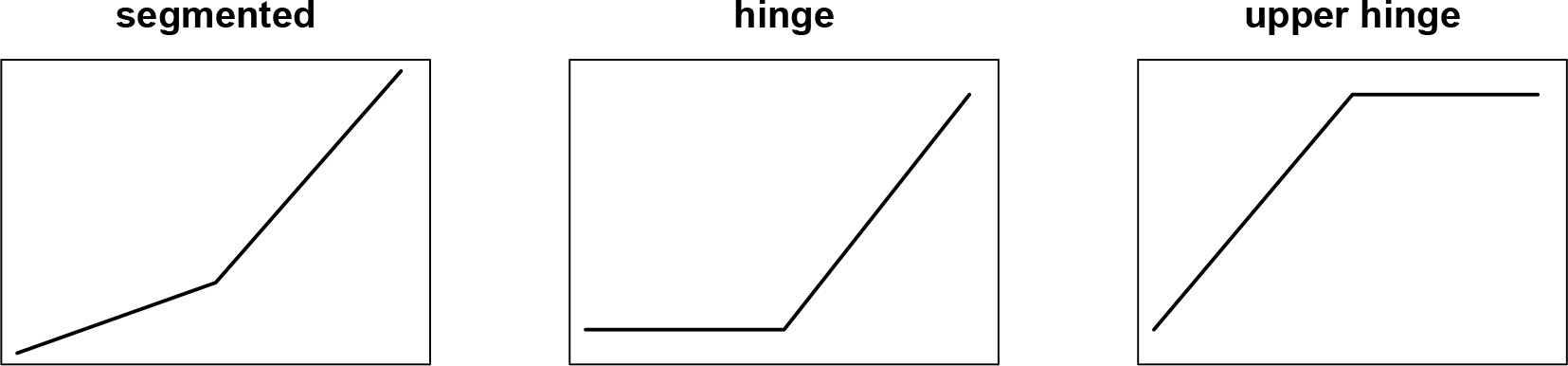
Three types of continuous threshold effects.

While upper hinge models offer a succinct summary of the relationship between the outcome and the predictor of interest, we do not expect them to exactly match the true data generating mechanisms except in some rare instances. Therefore, we wish to develop confidence interval methods that are robust to mean model misspecification. Bootstrap confidence intervals meet this criterion, but can be very slow if each model fit takes a long time. Previously, Fong (2018) developed a fast grid search algorithm for threshold linear models, which dramatically reduces the computational complexity when the sample size $n$ is large and the dimensionality of the predictor $p$ is small. In this paper we propose a new fast grid search algorithm that renders the algorithm from Fong (2018) inadmissible in the sense that the new algorithm is strictly better (Section 2). The performance of the new algorithm is especially impressive when $p$ is large.

For threshold logistic regression models and other threshold GLM of non-Gaussian families, there is no fast grid search algorithm available. To construct model-robust confidence intervals, we derive the asymptotic variance of the MLE without the assumption that the mean model is correctly specified (Section 3).

The proposed methods have been implemented in the R package chngpt, available from the Comprehensive R Archive Network, with key steps coded in C/C++. We carry out Monte Carlo studies in Section 4, present two real data examples from ecology in Section 5, and conclude the paper with a discussion in Section 6.

2. Fast grid search algorithm for upper hinge linear regression models

Finding the MLE of a threshold regression model is more difficult than usual due to the non-smoothness and non-convexity of the likelihood equation with respect to the threshold parameter. A common approach to dealing with such problem is to approximate the log-likelihood function with smooth functions (Pastor-Barriuso et al., 2003) or first order expansions (Muggeo, 2003). The approximation approaches generally lead to reasonable point estimates; however, bootstrapped confidence interval (CI) using smooth approximation can lead to substantial undercoverage in the case of threshold linear regression as shown by (Fong, 2018).

Without any form of approximating the overall likelihood function, we need to take a grid search approach. For any given candidate threshold value, the likelihood function of the corresponding submodel becomes smooth and convex, and hence easier to maximize. Once we find the likelihoods conditional on a grid of candidate threshold values, we can simply take the maximum of the set. The main disadvantage of the grid search approach is time. Previously Fong (2018) developed a fast grid search algorithm for threshold linear regression models that improved search performance by reusing key intermediate results from one submodel to the next. It reduced the computational complexity of step (4) in the algorithm below from $O\left(n{p}^2+p^3\right)$ to $O\left(p^3\right)$. When $p$ is small, the algorithm of Fong (2018) is extremely fast and makes it practical for data analysts to estimate bootstrap confidence intervals in routine use; but when $p$ is large, the algorithm slows down dramatically. Here we propose a new fast grid search algorithm that reduces the computational complexity of step (4) from $O\left(p^3\right)$ to $O\left(p\right)$. Furthermore, the proposed algorithm always outperforms Fong (2018) and renders the latter inadmissible.

For a given threshold value $e$, the log likelihood of the corresponding threshold linear regression submodel is proportional (with a negative constant of proportionality) to the residual sum of squares. This can be written as

$${\mathit{Y}}^T\left(\mathit{I}-{\mathit{H}}_e\right)\mathit{Y}={\mathit{Y}}^T\mathit{Y}-{\mathit{Y}}^T{\mathit{H}}_e\mathit{Y},\text{where}{\mathit{H}}_e\equiv {\mathit{X}}_e{\left({\mathit{X}}_e^T{\mathit{X}}_e\right)}^{-1}{\mathit{X}}_e^T,$$

${\mathit{X}}_e\equiv \left[\mathbf{1},\mathit{Z},(\mathit{x}-\mathbf{1}e{)}_{-}\right]$, $\mathbf{1}$ is a vector of $n$ 1’s $\mathit{x}$ is a vector of length $n$, $e$ is the (fixed) threshold value, and $\mathit{Y}$ is a vector of length $n$. Thus it will be sufficient to compare the different values of ${\mathit{Y}}^T{\mathit{H}}_e\mathit{Y}$, and choose the $e$ with the largest likelihood.

Computation of ${\mathit{H}}_e$ is somewhat computationally intensive, and can become cumbersome when performing a bootstrap. To speed up this computation, we consider the following formulation:

$${\mathit{X}}_e=\left[\mathit{X},{\mathit{v}}_e\right]\text{where}\mathit{X}\equiv [\mathbf{1},\mathit{Z}],\text{and}{\mathit{v}}_e\equiv (\mathit{x}-\mathbf{1}e{)}_{-}$$

Based on the matrix inversion formula when a column is added (Khan, 2008), we can write

$${\left({\mathit{X}}_e^T{\mathit{X}}_e\right)}^{-1}=\left[\begin{array}{cc}\mathit{A}+\frac{\mathit{A}{\mathit{X}}^T{\mathit{v}}_e{\mathit{v}}_e^T\mathit{X}{\mathit{A}}^T}{{\mathit{v}}_e^T{\mathit{v}}_e-{\mathit{v}}_e^{T}X\mathit{A}{\mathit{X}}^T{\mathit{v}}_e}& \frac{-\mathit{A}{\mathit{X}}^T{\mathit{v}}_e}{{\mathit{v}}_e^T{\mathit{v}}_e-{\mathit{v}}_e^T\mathit{X}A{\mathit{X}}^T{\mathit{v}}_e}\\ \frac{{\mathit{v}}_e^T\mathit{X}{\mathit{A}}^T}{{\mathit{v}}_e^T{\mathit{v}}_e-{\mathit{v}}_e^T\mathit{X}A{\mathit{X}}^T{\mathit{v}}_e}& \frac{1}{{\mathit{v}}_e^T{\mathit{v}}_e-{\mathit{v}}_e^T\mathit{X}A{\mathit{X}}^T{\mathit{v}}_e}\end{array}\right],\text{where}\mathit{A}\equiv {\left({\mathit{X}}^T\mathit{X}\right)}^{-1}$$

Letting $c_e\equiv {\mathit{v}}_e^T{\mathit{v}}_e-{\mathit{v}}_e^T\mathit{H}{\mathit{v}}_e$, where $\mathit{H}\equiv \mathit{X}\mathit{A}{\mathit{X}}^T$, we can now solve for:

$$\begin{gathered} {\mathit{H}}_e=\left[\begin{array}{ll}\mathit{X}& {\mathit{v}}_e\end{array}\right]c_e^{-1}\left[\begin{array}{cc}\mathit{A}{c}_e+\mathit{A}{\mathit{X}}^T{\mathit{v}}_e{\mathit{v}}_e^T\mathit{X}{\mathit{A}}^T& -\mathit{A}{\mathit{X}}^T{\mathit{v}}_e\\ {\mathit{v}}_e^T\mathit{X}{\mathit{A}}^T& 1\end{array}\right]\left[\begin{array}{c}{\mathit{X}}^T\\ {\mathit{v}}_e^T\end{array}\right] \\ =\mathit{X}\mathit{A}{\mathit{X}}^T+c_e^{-1}\left[\mathit{X}\mathit{A}{\mathit{X}}^T{\mathit{v}}_e{\mathit{v}}_e^T\mathit{X}{\mathit{A}}^T{\mathit{X}}^T-{\mathit{v}}_e{\mathit{v}}_e^T\mathit{X}{\mathit{A}}^T{\mathit{X}}^T-\mathit{X}\mathit{A}{\mathit{X}}^T{\mathit{v}}_e{\mathit{v}}_e^T+{\mathit{v}}_e{\mathit{v}}_e^T\right] \\ =\mathit{H}+c_e^{-1}\left[\left[\mathit{H}{\mathit{v}}_e\right]{\left[\mathit{H}{\mathit{v}}_e\right]}^T-{\mathit{v}}_e{\mathit{v}}_e^T\mathit{H}-\mathit{H}{\mathit{v}}_e{\mathit{v}}_e^T+{\mathit{v}}_e{\mathit{v}}_e^T\right] \\ =\mathit{H}+c_e^{-1}\left[\mathit{H}{\mathit{v}}_e-{\mathit{v}}_e\right]{\left[\mathit{H}{\mathit{v}}_e-{\mathit{v}}_e\right]}^T \end{gathered}$$

Note that $H$ does not change with $e$, and thus only needs to be computed once. Additionally, when computing the sum of squares, we find:

$$\begin{array}{l}{\mathit{Y}}^{\mathit{T}}{\mathit{H}}_e\mathit{Y}={\mathit{Y}}^{\mathit{T}}\left\{\mathit{H}+c_e^{-1}\left[\mathit{H}{\mathit{v}}_e-{\mathit{v}}_e\right]{\left[\mathit{H}{\mathit{v}}_e-{\mathit{v}}_e\right]}^{\mathit{T}}\right\}\mathit{Y}\\ ={\mathit{Y}}^{\mathit{T}}\mathit{H}\mathit{Y}+c_e^{-1}{\mathit{Y}}^{\mathit{T}}\left[\mathit{H}{\mathit{v}}_e-{\mathit{v}}_e\right]{\left[\mathit{H}{\mathit{v}}_e-{\mathit{v}}_e\right]}^{\mathit{T}}\mathit{Y}\\ =\underset{\text{independent}\text{of}e}{\underbrace{{\mathit{Y}}^{\mathit{T}}\mathit{H}\mathit{Y}}}+c_e^{-1}{\left({\mathit{Y}}^{\mathit{T}}[\mathit{H}-\mathit{I}]{\mathit{v}}_e\right)}^2\end{array}$$ (1)

Comparing this result with equation (3) of Fong (2018), we see that it allows us to replace inverting a $p\times p$ matrix with a series of multiplications.

The second term of equation (1) depends on ${\mathit{r}}^T{\mathit{v}}_e$, where $\mathit{r}=[\mathit{H}-\mathit{I}]\mathit{Y}$, and $c_e={\mathit{v}}_e^T{\mathit{v}}_e-{\mathit{v}}_e^T\mathit{H}{\mathit{v}}_e={\mathit{v}}_e^T{\mathit{v}}_e-{\mathit{v}}_e^T\mathit{B}{\mathit{B}}^T{\mathit{v}}_e$, where ${\mathit{B}}_{n\times p}=\mathit{X}{\left({\mathit{X}}^T\mathit{X}\right)}^{-1/2}$. All of ${\mathit{r}}^T{\mathit{v}}_e$, ${\mathit{B}}^T{\mathit{v}}_e$, and ${\mathit{v}}_e^T{\mathit{v}}_e$ involve taking the dot product of ${\mathit{v}}_e$ and some other vector or matrix. Consider ${\mathit{v}}_e$ for two successive values of $e$, $e_t$ and $e_{t+1}$, and suppose $e_t$ and $e_{t+1}$ correspond to the $k^{th}$ and $k+1^{th}$ ordered values of $x$. Assume that we have ordered the rows of the design matrix ${\mathit{X}}_e$ according to the ascending order of $x$, we find that ${\mathit{v}}_{e_{t+1}}-{\mathit{v}}_{e_t}=d_t{\mathit{\delta }}_t$, where $d_t\equiv e_{t+1}-e_t$, and ${\mathit{\delta }}_t$ is a vector of size $n$ with the first $k$ entries equal to $d_t$, and the remaining entries equal to zero. Thus, it follows that

$$\begin{array}{rr}{\mathit{v}}_{e_{t+1}}^T{\mathit{v}}_{e_{t+1}}& ={\mathit{v}}_{e_t}^T{\mathit{v}}_{e_t}-2{\mathit{\delta }}_t^T{\mathit{v}}_{e_t}+k{d}_t^2\end{array}$$ (2)

$$\begin{array}{}\\ {\mathit{v}}_{e_{t+1}}^T\mathit{r}& ={\mathit{v}}_{e_t}^T\mathit{r}-{\mathit{\delta }}_t^T\mathit{r}\\ \end{array}$$ (3)

$${\mathit{v}}_{e_{t+1}}^T\mathit{B}={\mathit{v}}_{e_t}^T\mathit{B}-{\mathit{\delta }}_t^T\mathit{B}.$$ (4)

We can use these relations to update the likelihood function of the submodel conditional on $e_{t+1}$ if we save the intermediate values ${\mathit{v}}_{e_t}^T{\mathit{v}}_{e_t}$, ${\mathit{v}}_{e_t}^T\mathit{r}$, and ${\mathit{v}}_{e_t}^T\mathit{B}$ while computing the likelihood function for the submodel conditional on $e_t$. We write this more formally as follows:

Algorithm 1.

The fast grid search algorithm for upper hinge linear regression

1.	Sort the samples by the ascending order of $x_i$.
2.	Compute and store ${\mathit{v}}_{e_1}^T{\mathit{v}}_{e_1}$, ${\mathit{v}}_{e_1}^T\mathit{r}$ and ${\mathit{v}}_{e_1}^T\mathit{B}$.
3.	Compute and store ${\mathit{Y}}^T\mathit{H}\mathit{Y}-{\mathit{Y}}^T{\mathit{H}}_{e_1}\mathit{Y}$ according to (1).
4.	For $t$ in 1 to $M-1$:
	(a) update ${\mathit{v}}_{e_{t+1}}^T{\mathit{v}}_{e_{t+1}}$, ${\mathit{v}}_{e_{t+1}}^T\mathit{r}$ and ${\mathit{v}}_{e_{t+1}}^T\mathit{B}$ according to (2), (3) and (4),
	(b) compute and store ${\mathit{Y}}^T\mathit{H}\mathit{Y}-{\mathit{Y}}^T{\mathit{H}}_{e_{t+1}}\mathit{Y}$ according to (1).

In step 4(a) of the above algorithm, we need to compute three sums ${\mathit{\delta }}_t^T\mathit{r},{\mathit{\delta }}_t^T\mathit{B}$, and ${\mathit{\delta }}_t^T\mathit{B}$. These sums can be simplified as:

$${\mathit{\delta }}_t^T\mathit{r}=d_t\sum _{i=1}^k{r}_i$$

$${\mathit{\delta }}_t^T{\mathit{v}}_{e_t}=d_t\left\{\left(\sum _{i=1}^k{x}_i\right)-k{e}_t\right\}$$

$${\mathit{\delta }}_{\mathit{t}}^T\mathit{B}=d_t\left[{\sum }_{i=1}^k{B}_{i,1}\cdots {\sum }_{i=1}^k{B}_{i,p}\right],$$

where $B_{i,j}$ refers to the $(i,j{)}^{th}$ element of the matrix $\mathit{B}$. Hence, we can compute the cumulative sums of ${\left\{r_i\right\}}_{i=1}^n$, ${\left\{x_i\right\}}_{i=1}^n$, ${\left\{B_{i,1}\right\}}_{i=1}^n,\cdots ,$ and ${\left\{B_{i,p}\right\}}_{i=1}^n$ upfront and simply do a look-up within the step (4) loop. The pseudocode for the entire implementation can be found in the Supplementary Materials Section A. An extension of the algorithm to handle weights is included in Section B of the Supplementary Materials.

Although we have described the proposed algorithm in the context of upper hinge linear regression models, the algorithm is generally applicable to other types of threshold linear regression models. This algorithm, however, only works for linear models; for other types of upper hinge regression models such as upper hinge logistic regression, we need a different practical approach to obtaining confidence intervals.

3. Asymptotic theory for upper hinge GLMs

For upper hinge GLMs that are not in the Gaussian family, we need to construct confidence intervals based on asymptotic theory. Let ${\ell }_{\mathit{\theta }}$ denote the log likelihood of the model. While ${\ell }_{\mathit{\theta }}$ is not differentiable with respect to $e$, its expectation is. Thus, we will study:

$$E_{XY\mathit{Z}}{\ell }_{\mathit{\theta }}=E_{X\mathit{Z}}\frac{m_0(X,\mathit{Z}){\eta }_{\mathit{\theta }}(X,\mathit{Z})-b\left\{{\eta }_{\mathit{\theta }}(X,\mathit{Z})\right\}}{\alpha }+E_{Y}c(y,\alpha )$$

Here, $m_0(X,\mathit{Z})$ denotes $E[Y\mid X,\mathit{Z}]$. When the model is misspecified, $m_0$ is an unknown function of $X,\mathit{Z}$.

Denote the maximizers of the empirical average log likelihood and its expected value by:

$${\stackrel{\mathit{ˆ}}{\mathit{\theta }}}_n\equiv \underset{\mathit{\theta }\in \Theta }{\mathrm{a}\mathrm{r}\mathrm{g}\mathrm{m}\mathrm{a}\mathrm{x}}{\mathbb{P}}_n{\ell }_{\mathit{\theta }}\text{and}{\mathit{\theta }}_0\equiv \underset{\mathit{\theta }\in \Theta }{\mathrm{a}\mathrm{r}\mathrm{g}\mathrm{m}\mathrm{a}\mathrm{x}}{E}_{XY\mathit{Z}}{\ell }_{\mathit{\theta }}$$

where ${\mathbb{P}}_n(\cdot )\equiv n^{-1}{\sum }_{i=1}^n(\cdot )$ denotes the empirical average. If the model is correctly specified, ${\mathit{\theta }}_0$ is the parameter of the data-generating mechanism. When the model is misspecified, ${\mathit{\theta }}_0$ corresponds to the parametric model that is closest to the true data generating mechanism as measured by the Kullback-Leibler divergence. The following proposition shows that the MLE is asymptotically normal under mild regularity conditions.

Proposition 1

If (i) the observations $\left(Y_i,X_i,{\mathit{Z}}_i\right)$ are i.i.d for $i=1,\dots ,n$; (ii) $E{X}^2<\mathrm{\infty }$, $E\parallel \mathit{Z}{\parallel }^2<\mathrm{\infty }$; $\Theta \subset R^{p+1}$ is compact and ${\mathit{\theta }}_0$ is unique; (iv) the distribution of $X$ is absolutely continuous and has density function $f_X(\cdot )$; and (v) $V_{{\mathit{\theta }}_0}$ is non-singular, then ${\stackrel{\mathit{ˆ}}{\mathit{\theta }}}_n\stackrel{p}{\to }{\mathit{\theta }}_0$. Furthermore,

$$\sqrt{n}\left({\stackrel{\mathit{ˆ}}{\mathit{\theta }}}_n-{\mathit{\theta }}_0\right)\stackrel{d}{\to }N(0,V_{{\mathit{\theta }}_0}^{-1}{\dot{\ell }}_{{\mathit{\theta }}_0}{\dot{\ell }}_{{\mathit{\theta }}_0}^T{V}_{{\mathit{\theta }}_0}^{-1}),$$

where

$${\dot{\ell }}_{\mathit{\theta }}={\alpha }^{-1}{E}_{X\mathit{Z}}\left(\left[m_0(X,\mathit{Z})-b^{\prime }\left\{{\eta }_{\mathit{\theta }}(X,\mathit{Z})\right\}\right]{\tilde{\mathit{X}}}_{\mathit{\theta }}\right),$$

with ${\tilde{\mathit{x}}}_{\mathit{\theta }}=\{1,{\mathit{z}}^T,(x-e{)}_{-},-I\{x<e\}{\beta }_{(x-e{)}_{-}}\}$, and

$$V_{\mathit{\theta }}=-{\alpha }^{-1}{E}_{XZ}\left[b^{\prime \prime }\left\{{\eta }_{\theta }(X,\mathit{Z})\right\}{\tilde{\mathit{X}}}_{\mathit{\theta }}{\tilde{\mathit{X}}}_{\mathit{\theta }}^T\right]+{\alpha }^{-1}\left[\begin{array}{ccc}[0{]}_{(p-1)\times (p-1)}& \underset{\_}{0}& \underset{\_}{0}\\ {\underset{\_}{0}}^T& 0& {\xi }_e\\ {\underset{\_}{0}}^T& \xi & {\zeta }_e\end{array}\right]$$

with

$${\xi }_e=-E_{X\mathit{Z}}\left\{\left[m_0(X,\mathit{Z})-b^{\prime }\left\{{\eta }_{\theta }(X,\mathit{Z})\right\}\right]I(X<e)\right\}$$

$${\zeta }_e=-{\beta }_{(x-e)-}{f}_X\left(e\right)E_{\mathit{Z}}\left[m_0(e,\mathit{Z})-b^{\prime }\left\{{\eta }_{\theta }(e,\mathit{Z})\right\}\right],$$

where $f_X\left(e\right)$ is the density function of $x$ evaluated at $e$, $\underset{\_}{0}$ is a vector of zeroes with length $p-1$, and $[0{]}_{(p-1)\times (p-1)}$ is a $(p-1)\times (p-1)$ matrix of zeroes.

The proof of Proposition 1 can be found in Section C of the Supplementary Materials. Using this result we can estimate the variance of the MLE to construct model-robust confidence intervals. It is worth noting that the most difficult-to-estimate term in the asymptotic variance is $E_{\mathit{Z}}{m}_0\left(e_0,\mathit{Z}\right)$. We estimate it by fitting a sufficiently flexible model to obtain an estimate of $m_0$ and use the empirical estimate $n^{-1}{\sum }_{i=1}^n{\hat{m}}_0\left(\hat{e},z_i\right)$.

4. Simulation studies

4.1. Speed of the proposed algorithm for upper hinge linear regression models

Table 1 compares the average run time of the algorithm from Fong (2018) and our proposed algorithm for for fitting an upper hinge linear regression model with $n=1000$. When $p=502$, we are not able to obtain a result for Fong (2018) because it takes too long. When $z$ is one-dimensional $(p=3)$, the method based on Fong (2018) takes an average of 1.3 seconds to fit an upper hinge linear regression model with 10³ bootstrap replicates; the method based on the proposed algorithm takes on average 0.88 seconds. The ratio of the run times between Fong (2018) and the proposed algorithm is 1.5 when $p=3$, the ratio increases with $p$ roughly on the order of $O\left(p\right)$. For example, as $p$ increases from 52 to 252, the ratio increases from 9.9 to 59.

Table 1:

Average and standard errors (in parentheses) of run time estimates for upper hinge linear model from 10³ Monte Carlo replicates. For each dataset, 10³ bootstrap replicates were performed to obtain confidence intervals. The design matrix X_e is of dimension 1000 × p.

p	Fong (2018)	Proposed	ratio
3	1.3 (0.0095)	0.88 (0.011)	1.5
12	8.2 (0.07)	3.2 (0.031)	2.5
52	250 (1.3)	25 (0.2)	9.9
252	20000 (74)	340 (1.4)	59
502		1400 (4.6)

4.2. Bias, coverage and efficiency of upper hinge linear regression model estimation

We study bias and coverage for upper hinge linear regression models in two settings. In the first setting, the true upper hinge model holds, with

$$y_i=z_i+{\left(x_i-3\right)}_{-}+{ϵ}_i,\text{where}{ϵ}_i~N(0,1).$$

In the second setting, the upper hinge model nearly holds, with

$$y_i=z_i+\left(x_i-3\right)-\mathrm{l}\mathrm{o}\mathrm{g}\left(1+\mathrm{e}\mathrm{x}\mathrm{p}\left(5\left(x_i-3\right)\right)/5+{ϵ}_i,\text{where}{ϵ}_i~N(0,1).\right.$$

Here, $Z$ is uniformly distributed over [−4, 4], and $X$ is uniformly distributed over [−1, 6]. In the upper hinge setting, we compare upper hinge and segmented model fits, and in the near upper hinge setting we compare model-based and bootstrap-based estimates of upper hinge model. For bootstrap, we choose the symmetric percentile method for estimating confidence intervals (Hansen, 2017) because the sampling distributions from a threshold model can be left-skewed for some parameters and right-skewed for others. We investigate sample sizes of 50,100, and 500. For the near upper hinge model, we approximate the parameter ${\mathit{\theta }}_0$ with parameter estimate from a single MonteCarlo run where $n=\mathrm{100,000}$. All simulations are carried out using 10,000 Monte Carlo (MC) replicates.

Table 2 shows the results when the true upper hinge model holds. Both segmented model fits and upper hinge model fits provide the right coverage. While there is little to no gain in precision of ${\beta }_z$ estimates when using the upper hinge model over the segmented model, the upper hinge model enjoys sizable advantage over the segmented model in the precision of ${\beta }_{(x-e{)}_{-}}$ estimates and threshold estimates. This can also be seen by comparing the the Monte Carlo distributions of ${\hat{\beta }}_{(x-e{)}_{-}}$ and $\hat{e}$ at $n=100$ in Figure 2(a) and by comparing the Monte Carlo distributions of the fitted curves in Figure 3(a). As sample size increases, this advantage gradually disappears in the case of ${\beta }_{(x-e{)}_{-}}$, but persists in the case of $e$. Intuitively, this contrast may be attributed to the fact that to estimate ${\beta }_{(x-e{)}_{-}}$, only the samples before the threshold matter. On the other hand, in estimating $e$, the uncertainty of the slope estimate after the threshold in a segmented model could have a negative impact.

Table 2:

Simulation results from 10,000 MC runs when the true model is an upper hinge linear model. Mean estimate, %bias, coverage, and MC SD of the parameter estimate are given for both the segmented and upper hinge models. Additionally, the ratios of the MC standard deviation of the parameter estimates from the two models fit are given.

		Segmented Model			Upper Hinge Model
	n	Est(%Bias)	Coverage	MC SD	Est(%Bias)	Coverage	MC SD	SD Ratio
${\mathit{\beta }}_z$
	50	1.00 (0)	0.945	0.07	1.00 (0)	0.941	0.06	1.02
	100	1.00 (0)	0.946	0.04	1.00 (0)	0.946	0.04	1.01
	500	1.00 (0)	0.944	0.02	1.00 (0)	0.945	0.02	1.00
${\beta }_{(x-e)-}$
	50	1.12 (12)	0.985	0.54	1.02 (2)	0.959	0.22	2.47
	100	1.04 (4)	0.977	0.19	1.01 (1)	0.961	0.13	1.44
	500	1.00 (0)	0.962	0.06	1.00 (0)	0.956	0.05	1.03
$e$
	50	2.97	0.968	0.84	3.01	0.950	0.50	1.69
	100	3.00	0.968	0.50	3.00	0.961	0.31	1.62
	500	3.00	0.962	0.19	3.00	0.956	0.13	1.45

Fig. 2:

Monte Carlo distributions of the estimated slope and parameter before the slope when the true model is an upper hinge model.

Fig. 3:

Monte Carlo distributions of the fitted curves when the true model is an upper hinge model. Left: upper hinge model fits, right: segmented model fits. Black lines are the truth.

Table 3 compares the performance of model-based and bootstrap confidence intervals when the near upper hinge model holds. While both model-based analytical and bootstrap confidence intervals provide the right coverage for ${\beta }_z$, only bootstrap confidence intervals do so for ${\beta }_{(x-e{)}_{-}}$ and $e$.

Table 3:

Simulation results from 10,000 MC runs when the true model is a near upper hinge linear model, and the data are fit using an upper hinge model. Mean estimate, %bias, and MC SD of the parameter estimate are given. Additionally, coverage and average standard error (SE) are given for model-based and bootstrap-based standard error estimates.

				Model-based		Bootstrap-based
	n	Est(%Bias)	MC SD	Coverage	SE	Coverage	SE
${\mathit{\beta }}_z$
	50	1.00 (0)	0.06	0.944	0.06	0.941	0.06
	100	1.00 (0)	0.04	0.949	0.04	0.946	0.04
	500	1.00 (0)	0.02	0.947	0.02	0.945	0.02
${\beta }_{(x-e)-}$
	50	1.02 (3)	0.22	0.898	0.17	0.959	0.28
	100	1.00 (2)	0.14	0.914	0.12	0.959	0.16
	500	0.99 (0)	0.06	0.916	0.05	0.952	0.06
$e$
	50	3.03	0.53	0.837	0.47	0.948	0.73
	100	3.02	0.34	0.880	0.32	0.958	0.49
	500	3.02	0.15	0.912	0.14	0.952	0.18

4.3. Bias, coverage and efficiency of upper hinge logistic regression model estimation

Similar to the linear case, we estimate the bias and coverage of the MLE for upper hinge logistic regression models in two settings, one when the true upper hinge model holds, and the other when the upper hinge model nearly holds. When the upper hinge model holds:

$$\mathit{Pr}\left(y_i=1\right)=\mathrm{expit}\left(z_i+{\left(x_i-3\right)}_{-}\right),$$

where expit is the inverse of the logit function, and when the near upper hinge model holds we have:

$$Pr\left(y_i=1\right)=\mathrm{e}\mathrm{x}\mathrm{p}\mathrm{i}\mathrm{t}\left(z_i+\left(x_i-3\right)-\mathrm{l}\mathrm{o}\mathrm{g}\left(1+\mathrm{e}\mathrm{x}\mathrm{p}\left(5\left(x_i-3\right)\right)/5\right)\right.$$

Again, $Z$ is uniformly distributed over [−4,4], and $X$ is uniformly distributed over [−1,6]. The marginal probability $y_i=1$ is 0.371 in the upper hinge setting, and 0.370 in the near upper hinge setting.

In the upper hinge setting, we fit both an upper hinge model and a segmented model, whereas in the near upper hinge setting we fit only the upper hinge model and compare model-based and model-robust variance estimates. We investigate sample sizes of 50, 100, 500, and 2000. The need to increase sample size up to 2000 is partly due to the fact that the finite sample bias of ${\hat{\beta }}_{(x-e{)}_{-}}$ is still relatively substantial when $n=500$. The simulation results from 10⁴ Monte Carlo replicates are summarized in Tables 4 and 5.

Table 4:

Simulation results from 10,000 MC runs when the true model is an upper hinge logistic model. Mean estimate, %bias, coverage, and MC SD of the parameter estimate are given for both the segmented and upper hinge models. The ratio of the MC standard deviation of the parameter estimates from the two models fit is given. The ratio of the MC interquartile range of the parameter estimates from the two model fits is also given.

		Segmented Model			Upper Hinge Model
	n	Est(%Bias)	Coverage	MC SD	Est(%Bias)	Coverage	MC SD	SD Ratio	IQR Ratio
${\mathit{\beta }}_{\mathit{z}}$
	50	1.39 (39)	0.989	0.68	1.29 (29)	0.985	0.57	1.19	1.12
	100	1.14 (14)	0.966	0.30	1.11 (11)	0.968	0.28	1.07	1.06
	500	1.02 (2)	0.952	0.09	1.02 (2)	0.953	0.09	1.01	1.01
	2000	1.00 (0)	0.951	0.05	1.00 (0)	0.951	0.05	1.00	1.00
${\beta }_{(x-e)-}$
	50	1.58 (58)	0.963	2.19	1.97 (97)	0.976	1.87	1.17	1.06
	100	1.51 (51)	0.939	1.69	1.45 (45)	0.949	1.23	1.38	1.21
	500	1.14 (14)	0.915	0.54	1.04 (4)	0.920	0.22	2.48	1.14
	2000	1.02 (2)	0.928	0.10	1.01 (1)	0.933	0.10	1.05	1.01
$e$
	50	3.05	0.923	1.44	2.99	0.919	1.28	1.12	1.23
	100	3.01	0.894	1.45	3.02	0.911	1.06	1.37	1.54
	500	3.01	0.908	0.74	3.02	0.931	0.43	1.72	1.52
	2000	3.00	0.934	0.28	3.00	0.938	0.20	1.43	1.37

Table 5:

Simulation results from 10,000 MC runs when the true model is a near upper hinge logistic model and the data are fit using an upper hinge model. Mean estimate, %bias, and MC SD of the parameter estimate are given. Additionally, coverage and average standard error (SE) are given for model-based and model-robust standard error estimates.

				Model-based		Model-robust
	n	Est(%Bias)	MC SD	Coverage	SE	Coverage	SE
${\mathit{\beta }}_{\mathit{z}}$
	50	1.28 (29)	0.57	0.986	0.42	0.959	0.63
	100	1.11 (12)	0.27	0.969	0.23	0.958	0.30
	500	1.02 (2)	0.09	0.953	0.09	0.95	0.09
	2000	1.00 (1)	0.05	0.947	0.05	0.946	0.05
${\beta }_{(x-e)-}$
	50	1.92 (95)	1.84	0.975	1.78	0.933	6.59
	100	1.45 (47)	1.22	0.954	0.74	0.953	3.83
	500	1.03 (4)	0.23	0.909	0.18	0.984	0.39
	2000	1.00 (1)	0.10	0.915	0.09	0.984	0.13
$e$
	50	3.01	1.31	0.914	1.53	0.788	7.81
	100	3.02	1.08	0.905	0.99	0.915	5.08
	500	3.03	0.47	0.919	0.42	0.992	0.99
	2000	3.03	0.22	0.922	0.21	0.987	0.37

The main conclusions are similar to those from the studies on linear regression, though some noteworthy differences exist. In Table 4, where the data generating model is truly upper hinge, the results again suggest that the upper hinge model allows more precise estimate of ${\beta }_{(x-e{)}_{-}}$ and $e$ (also see Figure 2(b), and Figure 3(b)) and that as sample size increases, the relative precision goes to 1 for ${\beta }_{(x-e{)}_{-}}$ but not for $e$. What is different from linear regression is that the relative precision does not change monotonically with sample size. The SE ratio peaks at $n=500$ and the interquartile range (IQR) ratio peaks at $n=100$. This complication is likely related to the relatively large finite sample bias observed, compared to that observed under linear regression scenarios.

Table 5 compares the performance of model-based and model-robust confidence intervals when the data generating model is nearly upper hinge. The results again show that model-based confidence intervals under-cover. Model-robust confidence intervals, on the other hand, seem to be conservatively large. This is likely due to the fact that in estimating model-robust asymptotic variance, we approximate $m_0$ by modeling the effect of $x$ with a natural cubic spline of two degrees of freedom. In Section 6, we discuss ways to improve the performance.

5. Real data examples

Threshold-related phenomena abound in ecology literature. Here we use two examples from population growth and impact of grazing on vegetation to illustrate the application of upper hinge models. Additional areas in which upper hinge models are especially applicable include body size (e.g. Sofaer et al., 2013) and density dependence (e.g. Thorne and Williams, 1999).

The first example documents the population growth of Paramecium caudatum, a single-celled protist that are naturally found in aquatic habitats, in laboratory culture (Neal, 2003; Gause et al., 1934). The dataset is available as part of the R assist package. Density-dependent population growth has traditionally driven the statistical development of nonlinear regression, in particular the sigmoid growth models. For our illustration we omit the data from day 0 to day 4, thus creating a scenario where only a partial growth curve dataset is available and it is difficult to fit a sigmoidal nonlinear model. Figure 4 plots the population density, measured as the mean number of individuals in 0.5 ml of medium from four independent experiments from day 5. Both upper hinge and segmented linear models provide good fits to the dataset. In the segmented model, the estimated slope after threshold is not significantly different from 0, 0.3 (95% CI: −2.0, 2.6); in both models, the estimated threshold is 10 with 95% bootstrap confidence interval between 8 and 12 (Table 6).

Fig. 4:

The paramecium population growth example. Left: upper hinge model fit; right: segmented model fit. Top: scatterplots with fitted lines; bottom: bootstrap distributions of the threshold estimate from 10³ replicates. The dashed lines correspond to the 95% symmetric bootstrap confidence interval.

Table 6:

Estimated slopes before and after the thresholds as well as the estimated thresholds from two real data examples. Left: estimates from the Paramecium population growth dataset; right: estimates from the responses of vegetation to grazing dataset. 95% bootstrap confidence intervals estimated from 10³ replicates are shown in parentheses.

	Paramecium growth		Response of vegetation to grazing
	upper hinge	segmented	upper hinge	segmented
before threshold	34.9 (22.0, 47.9)	34.3 (21.7, 47.0)	−0.268 (−0.415, −0.121)	−0.251 (−0.583, 0.081)
after threshold		0.3 (−2.0, 2.6)		−0.025 (−0.085, 0.034)
threshold	10 (8, 12)	10 (8, 12)	50.0 (25.0, 75.0)	50.0 (19.5, 80.5)

The second example concerns responses of vegetation to grazing in Mongolia rangelands (Sasaki et al., 2008). The dataset is available upon request from Dr. Sasaki. In the summer of 2006, the authors conducted field work in ten sites spanning both steppe and desertsteppe ecological zones. At each site, the authors identified sampling points at varying distances from a livestock camp or water source, which represented relative grazing intensity. At each sampling point, the aerial cover of all plant species within the sampled area is recorded. These plant species were classified into four different plant functional types: shrubs, grasses, perennial forbs, and annual forbs. In this example, we focus on annual forbs from site KD, a depression area in Kherlen Bayan Ulaan. Figure 5 shows that the annual forb cover decreases as grazing intensity decreases; this is because the foraging activities by livestock led to replacement of grass by annual forbs. Both upper hinge and segmented linear models provide good fits to the dataset. In the segmented model, the estimated slope after threshold is −0.025 with 95% bootstrap confidence interval between −0.085 and 0.034 (Table 6). The estimated slope before threshold is significantly different from 0 in the upper hinge model, −0.268 (95% CI: −0.415, −0.121), but not in the segmented model, −0.251 (95% CI: −0.583, 0.081), highlighting the advantage of upper hinge models. In both models, the estimated threshold is 50.0, but the upper hinge model has a slightly shorter confidence interval than the segmented model.

Fig. 5:

The responses of vegetation to grazing example. Left: upper hinge model fit; right: segmented model fit. Top: scatterplots with fitted lines; bottom: bootstrap distributions of the threshold estimate from 10³ replicates. The dashed lines correspond to the 95% symmetric bootstrap confidence interval.

6. Discussion

In this paper we formally introduced a new type of threshold models, upper hinge models, and studied its estimation and confidence intervals. We found that, compared to the more general segmented models, upper hinge models could be estimated with higher efficiency. For example, in the linear regression simulation study, the precision at which the slope before the threshold can be estimated from a dataset of size 100 in the upper hinge model is equal to the precision at which it can be estimated from a dataset of size 200 in the segmented model. In the real data examples, we also observed some improvement. In the example involving vegetation responses to grazing in Mongolian rangelands (Sasaki et al., 2008), the confidence interval for the slope before the threshold from the segmented model is more than twice as wide as that from the upper hinge model. The confidence interval for the threshold parameter is also longer in the segmented model than in the upper hinge model. In the example involving population growth of Paramecium caudatum (Neal, 2003; Gause et al., 1934), we did not observe improvement in estimation precision. The underlying cause of the difference between these two examples is not clear, although one possibility is the pattern of unexplained variability.

For model-robust confidence interval construction for upper hinge linear regression, we recommend using bootstrap confidence intervals and using grid search to find the MLE for each bootstrap dataset. We proposed a newer fast grid search algorithm, which makes this approach even more attractive in practice. For example, it takes only 0.21 seconds on a commodity CPU to fit an upper hinge linear regression model with 10³ bootstrap replicates for a dataset of size 500. The newer fast grid search algorithm works not only for upper hinge linear regression, but also for other types of threshold regression. We have implemented this new algorithm for segmented linear regression and hinge linear regression in the R chngpt package. The same idea can also be extended to discontinuous threshold linear regression models (e.g. Banerjee and McKeague, 2007), and potentially change-point problems (e.g. Rooch et al., 2019; Schnurr and Dehling, 2017). For upper hinge GLMs of families other than the Gaussian family, there is no fast grid search algorithm available for estimation. We recommend using approximation methods (Muggeo, 2003; Fong et al., 2017) to find MLE and using asymptotic theory to estimate model-robust confidence intervals. In simulation studies, we saw that such model-robust confidence intervals tended to overestimate the standard errors, which led to over-coverage. To get closer-to-nominal coverage, we could try to estimate $E_{\mathit{Z}}{m}_0\left(e_0,\mathit{Z}\right)$ better with more flexible nonparametric regression models as sample size increases. This, of course, makes the method less attractive for practical use. Research on fast grid search algorithms for threshold logistic regression models will be needed to improve inference for threshold logistic regression models.

In this paper we focus on single-threshold models, but many phenomena in ecological studies involve multiple thresholds, either within a single covariate or across multiple covariates. Study of multi-threshold models present an interesting future research direction. The computational burden for using a grid search approach to fit such models grows formidably as the size of the set of candidate thresholds values to be evaluated grows at the rate of $n^J$, where $J$ is the number of threshold parameters. In addition, theoretical challenges related to model identification also arise if multiple thresholds exist in a single covariate.

References

- Banerjee M and McKeague IW (2007). Confidence sets for split points in decision trees. The Annals of Statistics 35(2),543–574. [Google Scholar]
- Fong Y (2018). Fast bootstrap confidence intervals for continuous threshold linear regression. Journal of Computational and Graphical Statistics in press, 1–16. [DOI] [PMC free article] [PubMed] [Google Scholar]
- Fong Y, Huang Y, Gilbert P, and Permar S (2017). chngpt: threshold regression model estimation and inference. BMC Bioinformatics 18(1), 454–460. [DOI] [PMC free article] [PubMed] [Google Scholar]
- Gause GF et al. (1934). Experimental analysis of vito volterras mathematical theory of the struggle for existence. Science 79(2036),16–17. [DOI] [PubMed] [Google Scholar]
- Hansen BE (2017). Regression kink with an unknown threshold. Journal of Business and Economic Statistics 35(2),228–240. [Google Scholar]
- Hinkley DV (1971). Inference in two-phase regression. Journal of the American Statistical Association 66(336), 736–743. [Google Scholar]
- Khan M (2008). Updating inverse of a matrix when a column is added/removed. Technical report, Technical report, University of British Columbia, Vancouver. [Google Scholar]
- McCullagh P and Nelder J (1989). Generalized Linear Models, Second Edition. Monographs on Statistics and Applied Probability. Taylor & Francis. [Google Scholar]
- Muggeo V (2003). Estimating regression models with unknown break-points. Statistics in Medicine 22(19), 3055–3071. [DOI] [PubMed] [Google Scholar]
- Neal D (2003). Introduction to population biology. Cambridge University Press, Cambridge UK. [Google Scholar]
- Pastor R and Guallar E (1998). Use of two-segmented logistic regression to estimate change-points in epidemiologic studies. American journal of epidemiology 148(7),631–642. [DOI] [PubMed] [Google Scholar]
- Pastor-Barriuso R, Guallar E, and Coresh J (2003). Transition models for change-point estimation in logistic regression. Statistics in Medicine 22(7), 1141–1162. [DOI] [PubMed] [Google Scholar]
- Rooch A, Zelo I, and Fried R (2019). Estimation methods for the lrd parameter under a change in the mean. Statistical Papers 60(1),313–347. [Google Scholar]
- Sasaki T, Okayasu T, Jamsran U, and Takeuchi K (2008). Threshold changes in vegetation along a grazing gradient in mongolian rangelands. Journal of Ecology 96(1), 145–154. [Google Scholar]
- Schnurr A and Dehling H (2017). Testing for structural breaks via ordinal pattern dependence. Journal of the American Statistical Association 112(518), 706–720. [Google Scholar]
- Seber GA and Wild CJ (2003). Nonlinear regression. John Wiley & Sons, Hoboken, New Jersey. [Google Scholar]
- Sofaer HR, Chapman PL, Sillett TS, and Ghalambor CK (2013). Advantages of nonlinear mixed models for fitting avian growth curves. Journal of Avian Biology 44(5),469–478. [Google Scholar]
- Thorne SH and Williams HD (1999). Cell density-dependent starvation survival ofrhizobium leguminosarum bv. phaseoli: Identification of the role of an n-acyl homoserine lactone in adaptation to stationary-phase survival. Journal of bacteriology 181(3),981–990. [DOI] [PMC free article] [PubMed] [Google Scholar]
Associated Data
This section collects any data citations, data availability statements, or supplementary materials included in this article.