The social capital penalty paid by teetotallers

Abstract

Social capital is important and helps protect health and reduce loneliness. Governments worldwide are pursuing policies to reduce the amount of alcohol consumed to protect public health but alcohol consumption remains a prevalent feature of social interaction in the UK. Previous studies have identified a strong relationship between alcohol and social capital which varies in direction depending on the dimension of social capital studied.

Using a large nationally representative longitudinal dataset for the UK, we apply an outcome-wide longitudinal design for causal inference, adjusting for covariates, as well as lagged values of outcome and exposure, to investigate if drinking less alcohol or not drinking alcohol at all is related to five binary social capital outcomes: socialising, being active in an organization, feeling lonely, number of close friends, and a bridging social capital score. We use two drinking exposures, binary drinker status, and categorised drinking frequency.

We find that not drinking alcohol is negatively associated with socialising. Analysis using the frequency of drinking alcohol exposure finds drinking alcohol monthly or less is negatively associated with being active in an organisation. We find little evidence of any relationship between drinking alcohol and feelings of loneliness, number of friends and bridging social capital.

Our results suggest that non-drinkers face barriers to some forms of social capital including socialising, which could be due to alcohol being a social norm in the UK. However, our results also suggest that high-frequency drinkers can reduce their drinking with minimal impact on their social capital. Our findings suggest more needs to be done to make socialising easier for non-drinkers. Furthermore, our findings support the implementation of policies to reduce high-frequency drinking.

Highlights

• •Not drinking alcohol is negatively associated with socialising.
• •Relationship between not drinking and socialising specific to older individuals.
• •No differences in socialising between those who drink alcohol 4+ times per week and 2–4 times per month.
• •No evidence that not drinking alcohol is associated with loneliness or bridging social capital.

1. Background

Putnam (2000) argues that social links and connectedness are key for healthy flourishing societies. Putnam described these social connections as ‘social capital’. Putnam separated social capital into two distinct strands. Bonding – or exclusive – social capital refers to strong social ties between homogenous individuals (i.e. within families and/or existing networks of friends). Bridging – or inclusive – social capital refers to individuals and/or groups of individuals who attempt to expand social networks to include a more diverse social grouping.

There is a plethora of recent research that shows that high levels of social capital are beneficial for health (Bolin et al., 2003; Ehsan et al., 2019). Social capital can affect health through several channels including better equipping groups to participate in collaborative actions that benefit the wider community. Social capital can also affect health through promotion of positive social norms (of good health), promotion of beneficial health behaviours, and diffusion of information that is beneficial for health between the group members. More broadly, potential mechanisms between social capital and health include reduced loneliness and a greater sense of belonging. Social capital can empower people to take more of an interest in themselves, their friends/peers and their community which can lead to a ‘warm glow’ effect. Social capital, and in particular social participation, can affect health through decreased loneliness and increased empowerment. For example, people who participated in social groups in a deprived city in North West England had increased health and lower levels of health care utilisation (Munford et al., 2017, 2020) as well as higher levels of quality of life and reduced loneliness (Munford et al., 2020b).

Alcohol consumption is linked to a variety of poor health outcomes and there is a large global burden of disease attributable to its use (Global Burden of Disease 2016 Alcohol Collaborators, 2018). Because of its negative health effects, there has been a widespread increase in policymakers’ efforts to reduce alcohol consumption through methods such as taxation (Angus et al., 2019). Alcohol consumption decreased in most European countries between 1990 and 2017 (Manthey et al., 2019). For example, the non-drinking of alcohol amongst young people in Britain increased from 18% to 29% from 2005 to 2015 (Ng Fat et al., 2018). However, social culture in Britain is still dominated by alcohol, particularly in bars and public houses, which is seen as an instigator/focus of social activities (Smith & Foxcroft, 2009).

Leifman et al. (1995) found a U-shaped relationship between alcohol consumption and poor sociability with abstainers and heavy drinkers reporting the highest percentage of poor sociability. Previous research has found moderate benefits of alcohol consumption on socialization (Dare et al., 2014; Peele & Brodsky, 2000; Wilkinson & Dare, 2014).

Adams et al. (2022) found there was an income premium for drinking alcohol at social jobs (jobs that require greater social skills and social interaction), suggesting that this was due to the social capital formed by drinking alcohol.

Previous studies have found that specific proxies for social capital (such as higher trust) are negatively associated with drinking alcohol (Sjödin et al., 2022; Weitzman & Kawachi, 2000; Åslund & Nilsson, 2013). Other studies have found that some dimensions of social capital, such as joint activities with friends and neighbours, were associated with alcohol drinking behaviours (Pavlova et al., 2014; Seid, 2016). These studies used cross-sectional data so the direction of causality was unclear, and mostly used selected samples so may be less generalizable.

Pavlova et al. (2019) examined the relationship between volunteering in organisations and alcohol consumption using panel data. They found volunteering in organisations was related to an individual's alcohol consumption though this association between volunteering and drinking may reflect inter-individual differences. This study had many strengths but focused on one dimension of social capital and treated social capital as an exposure.

Platt et al. (2010) found mixed relationships between social support and alcohol drinking trajectories in older American adults; more frequent socialising with neighbours was associated with increased alcohol consumption while having close friends nearby was associated with decreased alcohol consumption. This study made strong use of longitudinal data but used a select cohort (ageing adults).

We may expect frequency of drinking alcohol to affect the social capital indicators considered in various ways. Theoretically it could have a positive effect on all of them. Given alcohol's ability to act as a ‘social lubricant’, drinking may make it easier for individuals to socialise and therefore see friends more often. Furthermore, given alcohol is often a norm for socialising in the UK, not drinking may exclude people from opportunities to socialise. Because of this, we may expect that reducing alcohol consumption could make it more difficult for an individual to join in with various social activities. For example, this may be seeing friends, or it could be participating in an organization or group.

Reduced socialising may make it harder for individuals to retain friends, so we might expect a reduction in alcohol consumption to lead to individuals having less friends. If individuals are less able to see friends or join in with social activities due to reduced alcohol consumption, we may observe that reduced alcohol consumption leads to individuals being less likely to actively participate in organisations.

A pathway through which we might expect reduced alcohol consumption to affect bridging social capital is that because of alcohol acting as a ‘social lubricant’ and reducing inhibitions, alcohol may lead to individuals feeling more comfortable socialising with individuals who are different to themselves, leading to increased bridging social capital.

Given the importance of social capital, it would be undesirable for reduced alcohol consumption to reduce an individual's social capital.

In this study, we use data from ‘Understanding Society’ to examine the relationship between alcohol consumption and five individual-level social capital outcomes in a British setting. Our study adds to the literature by estimating this relationship using longitudinal methods, with multiple individual-level social capital outcomes (both bonding and bridging) with a representative dataset.

2. Materials and methods

2.1. Data

2.1.1. Dataset

We use data from the UK Household Longitudinal Study: ‘Understanding Society’ (UKHLS). The UKHLS is a nationally representative household-level study of the UK population (University of Essex, ISER, 2020). UKHLS collects data on a wide range of participant characteristics including data on alcohol consumption and social outcomes.

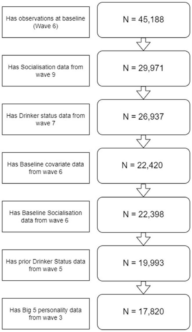
It has twelve waves of data; collected from 2009 to 2022. We use data from waves 3 (2011–2013), 5 (2013–2015), 6 (2014–2016), 7 (2015–2017) and 9 (2017–2019) due to these waves containing relevant variables on alcohol consumption, social capital outcomes, as well as covariates (see sections 2.1.2., 2.1.3, 2.1.4., and Fig. 1 below for further details).

Fig. 1.

Flow chart of variables and the waves they are derived from.

2.1.2. Exposures

We use two alcohol exposures, a binary exposure of not drinking alcohol in the past 12 months and a categorical exposure for frequency of drinking.

We initially estimate the extensive margin of the relationship between drinking alcohol and social capital using a binary exposure that indicates non-drinker status, derived from responses to the question ‘In the past 12 months have you taken an alcoholic drink?‘, participants could respond with ‘Yes’ or ‘ No’.

We then examine the intensive margin of the relationship between drinking alcohol and social capital using frequency of drinking alcohol as an exposure. Respondents were asked ‘Thinking about the past 12 months, how often do you have a drink containing alcohol?‘, potential responses included ‘Never’ (referent category), ‘Monthly or less’, ‘2–4 times per month’, ‘2–3 times per week’, and ‘4+ times per week’. For our prior exposure variable in the frequency of drinking alcohol analysis, we use different categories due to differences in the available responses in wave 5, the categories include ‘No’ (referent category), ‘Every 2 months or less’, ‘1–2 times a month’, ‘1–2 times a week’, or ‘3+ times a week’.

2.1.3. Outcomes

We use five outcomes related to social capital at the individual level; i) seeing friends socially when feels like it; ii) being active in an organisation; iii) never/rarely feeling lonely; iv) above median number of close friends; and v) above median bridging score. The first four outcomes arguably relate to ‘bonding’ social capital, while the fifth outcome relates to ‘bridging’ social capital. We make all of our outcomes binary to make it easier to compare the effect of reduced alcoholconsumption/stopping drinking across outcomes.

Our first outcome is a binary variable that indicates that an individual responded yes to the question ‘Do you go out socially or visit friends when you feel like it?‘.

Our second variable is a binary variable for being an active participant in an organisation. Respondents were asked if they participated in a variety of organisations, if they participate in any organisation the variable took a value of 1. Organisations include: political parties, trade unions, environmental groups, Parents'/School associations, tenants/residents' groups, religious/church organisations, voluntary services, pensioners' organisations, scouts/guides, professional organisations, other community groups, social/working men clubs, sports clubs, WI/townswomen's guilds, women's group/female organisations, or ‘other’.

Though the list of organisations is quite diverse, and drinking alcohol may be a social norm for some organisations while others might not, we group them together as we are interested in estimating if not drinking alcohol is associated with reduced likelihood of organization participation, not which type of organization an individual participates in.

We choose to focus on a binary variable for being in one organisation as opposed to a count variable relating to the number of organisations an individual participates in. We do this because we believe the marginal benefits of being in one group as opposed to zero is much larger than the marginal benefits of being in, for example, five groups instead of four; that is, the extensive margin of participation is greater than the intensive margin of participation. Furthermore, we use a binary indication of participation in any group rather than the count of all groups participated in as there is evidence that different people classify the same group membership in different ways (see, for example, Munford et al. (2017)). Therefore, the count may lead to different values for people who attend the same groups.

Our third outcome relates to loneliness. Individuals were asked ‘How often do you feel lonely?‘. If they responded ‘Never/rarely’, the variable took a value of 1, otherwise, if they responded ‘sometimes’ or ‘often’, the variable took a value of 0. Though loneliness is not necessarily a dimension of social capital, previous research has found it to be associated with social capital, with an intervention to increase social capital leading to reduced loneliness (Coll-Planas et al., 2017). Furthermore, loneliness can be viewed as a discrepancy between the desired amount of social interaction (a dimension of social capital) and the actual amount of social interaction an individual has (Algren et al., 2020).

Our fourth outcome variable is a binary variable for having above the median number of close friends (4 close friends). Individuals reported the number of close friends they had as a count variable.

Our final outcome variable relates to bridging social capital and looks at whether an individual's ‘bridging score’ is above or below the median (3 or higher, where the score takes values 0–4). Our bridging score is operationalized by the number of different characteristics to the individual that are represented in their social network. This score attempts to capture the same dimension of bridging social capital as ‘the contact with similar/different people’ dimension of the survey constructed by Villalonga-Olives et al. (2016).

The bridging score is constructed from responses to questions posed to individuals about what proportion of their friendship group is similar to them with regard to ethnicity, age, income and education, data from these questions have been used to capture bridging social capital in previous studies (Collischon & Eberl, 2021) . A higher bridging score indicates an individual has a more diverse set of friends.

The bridging score increases by 1 for every characteristic that has diverse representation in an individual's set of friends e.g. if an individual has a friend who is of different race to themselves, their bridging score increases by 1 point. The components of our bridging score and how they contribute to the total score are detailed in Table 1.

Table 1.

Construction of Bridging score.

Bridge score component	Question in survey	Score
		0	1
Ethnicity	What proportion of your friends are of the same ethnic group as you?	“All similar”	“More than half”, “about half”, or ‘less than half”
Age	What proportion of your friends are of a similar age as you?	“All similar”	“More than half”, “about half”, or ‘less than half”
Income	What proportion of your friends have a similar level of education as you?	“All similar”	“More than half”, “about half”, or ‘less than half”
Education	What proportion of your friends have similar incomes to you?	“All similar”	“More than half”, “about half”, ‘less than half”

Notes: Our Bridging score takes values between 0 and 4, is calculated from the sum of 4 scores from individual Bridge score components (0 being worst, 4 being best).

2.1.4. Covariates

We control for characteristics that feasibly relate to alcohol consumption and social capital, including age, gender, ethnicity, having a child under 16 and employment status. Additionally, we also control for social class using monthly household income and educational attainment.

We control for physical and mental health using self-assessed health, the physical health component of the 12 question version of the short form health questionnaire (SF-12), and the General Health Questionnaire subjective well-being score (GHQ-12). The SF-12 is a validated generic health status questionnaire that is often used in surveys, we use a constructed score ranging from 0 to 100 (100 indicating high physical function) (Jenkinson et al., 1997). The GHQ-12 subjective well-being score uses data from the 12 questions to construct a likert score ranging from 0 to 36 (36 indicating highest level of distress) (Böhnke & Croudace, 2016; Goldberg & Williams, 1988).

We further include a proxy for diet through the number of days per week an individual eats fruit and vegetables.

We further control for ‘Big Five’ personality traits, as measured by the Big Five Inventory (a self-report inventory) (Benet-Martínez & John, 1998; John et al., 1991, 2008). The Big Five personality traits are a grouping of personality traits into five dimensions or traits, these traits are agreeableness, conscienctiousness, extraversion, neuroticism, and openness (Goldberg, 1990). They are a method of quantifying personality types and are often used in the social sciences.

We also include a number of controls that VanderWeele et al. (2020) suggest social science studies should generally control for; including neighbourhood social cohesion, smoking, ethnicity, political affiliation, and whether diagnosed with depression.

Data for our covariates come from wave 6, except for the ‘Big Five’ personality traits, and how often an individual eats fruit and vegetables, which come from waves 3 and 5 respectively.

2.2. Empirical strategy

2.2.1. Outcome-wide longitudinal design for causal inference

We structure our analysis using the outcome-wide longitudinal framework specified by VanderWeele et al. (2020). We include many covariates to reduce the risk of our estimated effect of exposure being affected by omitted variable bias.

We utilise the longitudinal nature of the dataset and structure our data such that covariate data is collected at a time point before exposure data, which is collected at a time point prior to outcome data (Fig. 1). Further explanation of the outcome-wide longitudinal framework can be found in appendix 1. Fig. 1 shows a flowchart of variables and the waves they are derived from.

Controlling for covariates from a period that precedes exposure reduces the risk of accidently controlling for a mediator of exposure and outcome which would lead to a biased estimate of the relationship between exposure and outcome. Where possible, we also control for outcome at baseline to help mitigate the risk of reverse causation. We further control for pre-baseline exposure to reduce the risk of reverse causality and confounding (VanDerWeele et al., 2020).

We perform multiple logistic regression models with different outcome variables using data from wave 9, exposure data from wave 7, covariate data from wave 6, prior outcome data from wave 6, and prior exposure data from wave 5 (Fig. 1). Due to data limitations, we do not control for baseline outcomes for models that use loneliness as an outcome. We use a Bonferroni correction to adjust for multiple testing and divide our p-value thresholds by five.

2.2.2. E-values

As a form of sensitivity analysis, we calculate E-Values for our point estimates and confidence intervals. E-values are a measure of robustness against unadjusted confounding (VanderWeele et al., 2020). VanderWeele and Ding (2017) define E-Values as the ‘minimum strength of association, on the risk ratio scale, that an unmeasured confounder would need to have with both the exposure and the outcome to fully explain away a specific exposure-outcome association, conditional on the measured covariates.‘.

E-values require minimal assumptions and are reliant on the magnitude of the association between the exposure and outcome, so, unlike p-values, cannot be made arbitrarily small by increasing sample size (VanderWeele & Ding, 2017).

The lowest possible E-Value is 1, which indicates no un-measured confounding is required to explain away the exposure-outcome relationship, higher values indicate higher robustness to confounding.

We use the formula for E-values specific to odds ratios (OR), specified in appendix 3 (VanderWeele & Ding, 2017). Empirical proofs for E-values can be found in Ding and VanderWeele (2016). We use the E-Value calculator created by Mathur et al. (2018).

2.2.3. Regression analysis

Equation (1) details our estimation strategy.

$${\mathrm{Y}}_{\mathrm{i}9}=\tau {\mathrm{A}}_{\mathrm{i}\mathrm{j}7}+\rho {\mathrm{A}}_{\mathrm{i}\mathrm{j}5}+\delta {\mathrm{Y}}_{\mathrm{i}6}+{\mathrm{B}\mathrm{X}}_{\mathrm{i}6}+{\mathrm{u}}_{\mathrm{i}}$$ (1)

where Y_i9 represents our social capital outcome for individual ‘i’ in wave 9, A_ij7 represents the alcohol exposure in wave 7 (post-baseline), A_ij5 represents the pre-baseline value of alcohol exposure (in wave 5), Y_i6 represents a baseline value of the outcome (from wave 6), X_i6 is our vector of baseline covariates and u_i represents our random error for individual ‘i’. The superscript ‘j’ indicates which exposure we are using, j=1 indicates a binary drinker/non-drinker (extensive margin) exposure, and j=2 indicates frequency of alcohol consumption (intensive margin) exposure. Our coefficient of interest is $\tau$, which conditional on assumptions holding, represents the effect of not drinking or drinking less frequently on later social capital outcomes.

We estimate our results using logistic regression with robust standard errors. We report the point estimate adjusted odds ratio for our exposure, the E-Value for the point estimate, and the E-Value for the 95% confidence interval.

Because the relationship between not drinking and social capital outcomes might differ by age and sex, we conduct additional analysis where we stratify our analysis that uses a binary does not drink outcome by sex, and by age (under 35/35 or over at baseline) to create 4 sub-groups.

Our analysis was conducted using Stata 14 (StataCorp, 2015).

3. Results

3.1. Descriptive statistics

Table 2 presents descriptive statistics on the analysis sample. Approximately 87% of our sample were visiting friends socially when they wanted to in our outcome wave (wave 9). 16% of our sample were not drinking at the time of exposure (wave 7), and the most populated frequency of drinking alcohol category was ‘2–3 times a week’ (24.3%). The average age of our sample in wave 6 was 51.7. Our sample was mostly female (57.3%) and white (91.5%). 70.1% of our sample were married, and 31% of our sample had a child aged 16 or under at baseline. The average monthly net-household income for our sample was £3447.45 per month. 42.6% of our sample were at least degree educated and most of our sample was in work (60%).

Table 2.

Descriptive statistics of sample (N = 17,820).

	Mean/%	S.D.
Outcome (Wave 9)
Goes out socially or visit friends when feels like it	0.87	0.34
Active in organisation	0.5	0.5
Never feels lonely	0.66	0.47
Number of close friends	5.49	7.07
Number of close friends above median (>=5)	0.48	0.5
Bridging score	2.58	1.24
Bridging score above median (>=3)	0.57	0.49
Exposure (Wave 7)
Drinker/non-drinker (Non-drinker = 1)	0.16	0.37
Alcohol frequency (Wave 7)
4+ times a week	14.8%
2–3 times a week	24.3%
2–4 times a month	23.6%
Monthly or less	21.1%
Never	16.3%
Baseline Outcome (Wave 6)
Goes out socially or visit friends when feels like it	0.89	0.32
Active in organisation	0.53	0.5
Number of close friends	5.25	7.66
Number of close friends above median (>=5)	0.45	0.5
Bridging score	2.66	1.21
Bridging score above median (>=3)	0.6	0.49
Prior exposure (Wave 5)
Does not drink	0.16	0.36
How often have you had an alcoholic drink during the last 12 months
3+ times a week	27.8%
1–2 times a week	25.6%
1–2 times a month	14.9%
Every 2 months or less	16.1%
No	15.6%
Covariates (Wave 6)
Highest educational qualification
No Education	8.7%
Other	9.1%
GCSE	19.4%
A-Level	20.2%
Degree	42.6%
Total household net income - no deductions	3447.45	5321.18
Age	51.7	15.85
Sex
Male	42.7%
Female	57.3%
Urban/rural
Urban	72.6%
Rural	27.4%
Self-assessed health
Excellent	17.3%
very good	37.2%
Good	28.1%
Fair	13.3%
Poor	4.2%
Marital status
Married/Cohabiting	70.1%
Widowed	5.8%
Separated/Divorced	9.2%
Never Married	14.8%
Has child aged 16 or under	0.31	0.46
Cares for elderly or sick person	0.21	0.41
Subjective wellbeing (GHQ): Likert	10.67	5.2
SF-12 Physical Component Summary (PCS)	49.88	10.84
Religion
Atheist	41.6%
Christian	48.0%
Muslim	2.6%
Other	7.8%
Ethnicity
White	91.5%
Mixed race	1.3%
Asian	4.7%
Black	2.1%
Other	0.4%
In employment	0.6	0.49
Days each week eat fruit
Never	5.8%
1–3 days	24.9%
4–6 days	18.7%
every day	50.5%
days each week eat vegetables
Never	1.3%
1–3 days	16.1%
4–6 days	26.9%
every day	55.7%
Neighbourhood Social Cohesion,(α= .78)	15	2.52
Number of close friends	5.25	7.66
Big 5 personality trait: Agreeableness	5.64	1.01
Big 5 personality trait: Conscientiousness	5.53	1.07
Big 5 personality trait: Extraversion	4.58	1.3
Big 5 personality trait: Neuroticism	3.55	1.42
Big 5 personality trait: Openness	4.58	1.27
Government Office Region
North East	4.2%
North West	10.4%
Yorkshire and the Humber	7.7%
East Midlands	7.7%
West Midlands	7.9%
East of England	9.2%
London	8.6%
South East	13.1%
South West	9.7%
Wales	6.7%
Scotland	9.7%
Northern Ireland	5.2%
Smoker	0.14	0.35
Political allegiance
Unknown party/other party	43.7%
Conservative/right-wing	26.0%
Left/centre-left	26.0%
Centrist	4.3%
Has been diagnosed with depression before	0.09	0.28

3.2. Outcome-wide longitudinal design for causal inference framework results

In this section we will present the results for each outcome. The results for our main analyses can be found in Table 3, results for our additional stratified analyses can be found in Table 4. The associations between our covariates and outcomes for both the extensive and intensive margin analysis can be found in appendix 5.

Table 3.

Outcome-wide longitudinal framework results.

	Goes out socially when feels like it		Active in organization		Never lonely a		Close friends >= 5		Bridging score >= 3
	Coefficient + 95% C.I.	E-Value	Coefficient + 95% C.I.	E-Value	Coefficient + 95% C.I.	E-Value	Coefficient + 95% C.I.	E-Value	Coefficient + 95% C.I.	E-Value
Extensive margin
Does not drink alcohol	0.65***	2.44	0.86e*	1.37	0.97	1.15	0.85e*	1.39	0.96	1.17
	[0.56,0.77]	1.93	[0.76,0.97]	1.13	[0.85,1.10]	1	[0.75,0.97]	1.15	[0.82,1.12]	1
Drinking frequency (Referent = 4+ times a week)
2-3 times a week	1.06	1.31	0.93	1.24	0.98	1.12	1.02	1.1	0.92	1.25
	[0.88,1.27]	1	[0.82,1.05]	1	[0.86,1.11]	1	[0.90,1.14]	1	[0.81,1.06]	1
2-4 times a month	1.04	1.26	0.91	1.27	0.89	1.31	1.05	1.18	0.97	1.13
	[0.84,1.30]	1	[0.79,1.05]	1	[0.77,1.03]	1	[0.91,1.21]	1	[0.83,1.14]	1
Monthly or less	0.78e*	1.87	0.81*	1.47	0.81e*	1.47	0.93	1.23	0.95	1.2
	[0.62,0.99]	1.11	[0.69,0.95]	1.19	[0.68,0.95]	1.18	[0.79,1.09]	1	[0.79,1.14]	1
Does not drink	0.63**	2.54	0.75*	1.57	0.87	1.36	0.87	1.34	0.91	1.27
	[0.49,0.82]	1.74	[0.63,0.90]	1.29	[0.71,1.05]	1	[0.73,1.05]	1	[0.73,1.14]	1
Range of N	17813–17820		17314–17321		17531–17538		17258–17264		12540–12544

Note: e* p < 0.05, *p < 0.01, **p < 0.002, ***p < 0.0002. The adjusted Odds ratio associated with each variable are displayed. 95% confidence intervals are in brackets. E-values for coefficient and 95% confidence interval can be found in the column to the right. Covariates include; Highest educational qualification, total household net income, age, sex, urban/rural, self-assessed health, marital status, has child aged 16 or under, carer status, GHQ, religion, ethnicity, employed/non-employed, SF-12 Physical Component Summary (PCS), days each week eat fruit, days each week eat vegetables, Neighbourhood Social Cohesion, Number of close friends, Agreeableness (Big 5), Conscientiousness (Big 5), Extraversion (Big 5), Neuroticism (Big 5), Openness (Big 5), Government Office Region, whether smokes, political allegiance, and whether diagnosed with depression before.

^aIndicates that models with this outcome do not include past value of outcome as a covariate.

Table 4.

Outcome-wide longitudinal framework, extensive margin, stratified by age and sex.

Sample	Exposure	Goes out socially when feels like it		Active in organization		Never lonely a		Close friends >= 5		Bridging score >= 3
		Coefficient + 95% C.I.	E-Value	Coefficient + 95% C.I.	E-Value	Coefficient + 95% C.I.	E-Value	Coefficient + 95% C.I.	E-Value	Coefficient + 95% C.I.	E-Value
Male & Age <35 (N = 978 – 1185)	Does not drink alcohol	0.76	1.95	1.45	1.7	0.97	1.15	0.88	1.34	1.78	2
		[0.39,1.49]	1	[0.83,2.55]	1	[0.56,1.66]	1	[0.48,1.61]	1	[0.92,3.46]	1
Male & Age >=35 (N = 4454–6248)	Does not drink alcohol	0.65*	2.44	0.83	1.43	0.95	1.18	0.89	1.32	1.08	1.23
		[0.49,0.88]	1.54	[0.66,1.05]	1	[0.73,1.24]	1	[0.70,1.12]	1	[0.79,1.48]	1
Female & Age < 35 (N = 1370–1710	Does not drink alcohol	0.73	2.1	0.70	1.68	0.95	1.19	0.93	1.24	0.87	1.35
		[0.45,1.18]	1	[0.48,1.01]	1	[0.67,1.35]	1	[0.64,1.35]	1	[0.58,1.32]	1
Female & Age >= 35 (N = 5740–8495)	Does not drink alcohol	0.63***	2.58	0.87	1.36	1.01	1.09	0.82e*	1.44	0.86	1.37
		[0.50,0.79]	1.86	[0.73,1.03]	1	[0.85,1.21]	1	[0.69,0.98]	1.13	[0.70,1.07]	1

Note: e* p < 0.05, *p < 0.01, **p < 0.002, ***p < 0.00.

02. Table shows extensive margin analysis (does not drink alcohol as exposure), stratified by sex, and stratified again by age. The adjusted Odds ratio associated with each variable are displayed. 95% confidence intervals are in brackets. E-values for coefficient and 95% confidence interval can be found in the column to the right. Covariates include; Highest educational qualification, total household net income, age, sex, urban/rural, self-assessed health, marital status, has child aged 16 or under, carer status, GHQ, religion, ethnicity, employed/non-employed, SF-12 Physical Component Summary (PCS), days each week eat fruit, days each week eat vegetables, Neighbourhood Social Cohesion, Number of close friends, Agreeableness (Big 5), Conscientiousness (Big 5), Extraversion (Big 5), Neuroticism (Big 5), Openness (Big 5), Government Office Region, whether smokes, political allegiance, and whether diagnosed with depression before.

^aIndicates that models with this outcome do not include past value of outcome as a covariate.

3.2.1. Sees friends socially when feels like it

We find that not drinking alcohol is strongly associated with decreased odds of social interaction, with an aOR (adjusted odds-ratio) of 0.65 (P.E. E-value: 2.44, 95% C.I. E-value: 1.93) (Table 3).

Our drinking alcohol frequency analysis finds no evidence of drinking alcohol 2–3 times per week or 2–4 times per month having any association with social interaction relative to drinking 4+ times per week (Table 3). Not drinking alcohol had an aOR of 0.63 (P.E. E-value: 2.54, 95% C.I. E-value: 1.74) relative to drinking 4+ times per week (Table 3).

Stratified analysis suggests that the relationship between not drinking and socialising may be age specific, with not drinking being associated with decreased odds of social interaction in men over 35 (aOR: 0.65, P.E. E-Value: 2.44, 95% C.I. E-value: 1.54), and women over 35 (aOR: 0.63, P.E. E-Value: 2.58, 95% C.I. E-value: 1.86), while no significant association is observed for men and women under 35 (Table 4).

3.2.2. Active in organisation

After adjusting for multiple testing, we find no significant association between not drinking alchol (relative to being a drinker) and being active in an organisation (Table 3).

Our drinking alcohol frequency analysis finds some evidence of a negative intensive margin between lower alcohol drinking frequency and being active in an organisation (Table 3). Drinking alcohol monthly or less is associated with being less likely to be active in an organization relative to drinking alcohol 4+ times per week, with an aOR of 0.81 (P.E. E-value: 1.47, 95% C.I. E-value: 1.19) (Table 3). Not drinking alcohol (relative to drinking 4+ times per week) is also associated with being less likely to be active in an organization, with an aOR of 0.75 (P.E. E-value: 1.57, 95% C.I. E-value: 1.29) (Table 3).

Stratified analyses finds some evidence of age and sex having an impact on the relationship between not drinking alcohol and being active in an organization, but the association between not drinking alcohol and being active in an organisation is insignificant for each stratified group (Table 4).

3.2.3. Loneliness score

After adjusting for multiple testing, we find little evidence of not drinking alcohol, or reduced frequency of alcohol consumption having any association with loneliness (Table 3).

Stratified analyses finds little evidence of the relationship between not drinking alcohol and loneliness being impacted by age or sex (Table 4).

3.2.4. Number of close friends

After adjusting for multiple testing, we find little evidence of not drinking or drinking alcohol less frequently having any relationship with number of close friends (Table 3).

Analyses using stratified samples finds little evidence of the relationship between not drinking and number of close friends being impacted by age or sex (Table 4).

3.2.5. Bridging score

We find little evidence of not drinking alcohol or lower alcohol drinking frequency having any association with bridging social capital (Table 3).

Stratified analyses finds some differences in the magnitude of the relationship between not drinking alcohol and bridging social capital, with the coefficient being positive for men under 35 (aOR: 1.78), but negative for women under or over 35, though none of the estimated relationships are significant (Table 4).

4. Discussion

Our results suggest that not drinking alcohol has mixed effects on social capital, and this varies with the type of social capital and the dimension of the type of social capital. We further find that we observe differences in results at the extensive margin (drinking/not drinking alcohol), and the intensive margin (frequency of alcohol drinking).

We find evidence that, in a British setting, not drinking alcohol has potentially adverse effects on social interactions. We find a strong negative relationship between not drinking alcohol and our measure of socialising, which agrees with previous studies that found social interaction measures to correlate with alcohol consumption (Pavlova et al., 2014; Seid, 2016). However, we find no significant differences in socialising between drinking 4+ times per week, 2–3 times per week, or 2–4 times per month.

We find some evidence that not drinking alcohol, or drinking alcohol monthly or less is associated with being less likely to be in an organization relative to our highest alcohol-drinking category. However, the E-values on these estimates were low. This finding is somewhat in line with the findings of Seid (2016).

However, not drinking alcohol does not have noticeable disadvantages with regard to other dimensions of bonding social capital; we find little evidence that not drinking alcohol is associated with loneliness or having less than the median number of friends.

We further find little evidence that not drinking alcohol has any adverse effect on bridging social capital suggesting that while drinking alcohol may somewhat improve bonding capital, it does not facilitate inter-group interaction.

Stratified analysis finds that the relationship between not drinking alcohol and socialising may vary by age, with there being no evidence of an association in those under the age of 35 at baseline, but strong evidence of an association in those aged 35 or over at baseline. This could be a result of younger individuals being less likely to drink alcohol generally and therefore socialising with peers being less likely to involve drinking, making socialising more accessible to non-drinkers.

The reason for our finding of a negative relationship between not drinking alcohol and socialising could be due to alcohol being the norm for socialization in the UK, and that not drinking alcohol limits the number of opportunities for social interactions (e.g. pub trips). Alternatively, it could be because alcohol acts as a ‘social lubricant’ and makes it easier for individuals to socialise and stopping drinking alcohol causes individuals to socialise less.

However, there is always the possibility our findings are due to reverse causality, with individuals making decisions/life choices that lead to seeing friends less. Then, if drinking alcohol is a by-product of seeing friends, they will end up drinking alcohol less. This would be in line with the findings of Wilkinson et al. (2012) who found in a mixed-methods study that retired adults began to drink more as they had more leisure time to socialise. By utilising longitudinal methods, and including a baseline value of the outcome, we have somewhat mitigated the risk of our findings being affected by reverse causality (VanderWeele et al., 2020).

4.1. Policy implications

Our research suggests the need for an increased emphasis on non-alcohol-related social activities in the UK to ensure that those who have chosen not to drink do not have to face a limited social life. Due to the adverse effects that alcohol has on health, we do not recommend individuals increase the amount they drink to improve social outcomes and feel it is the duty of policymakers and others to make socialising more accessible to non-drinkers.

Furthermore, our findings suggest that there are no differences in socialising between those who drink 4+ times a week, and those who drink 2–3 times per week or 2–4 times per month. This suggests that frequent drinkers could cut down the frequency they drink without impacting their ability to socialise. When combined with the limited evidence of association between drinking and other social capital outcomes, our findings support policies aimed at reducing high frequency drinking and drinking in general, such as taxation of alcohol and public information campaigns promoting awareness of the harms of alcohol.

4.2. Strengths and limitations

Our study has several strengths. Because of the richness of the data, we can look at the relationship between alcohol and a variety of social capital outcomes, both bonding and bridging. We are further able to control for many covariates, reducing the risk of unobserved confounding.

Because the dataset is longitudinal, we are also able to temporally order our covariates, exposure, and outcome, and can control for prior values of exposure and outcome, allowing us to reduce the risk of our results being affected by reverse causality.

However, our study also has weaknesses due to the nature of the dataset; we are not able to construct a continuous variable that looked at the frequency of social interactions. We also do not identify potential mediators and moderators of the relationship between alcohol consumption and socialising. Furthermore, our sample is relatively old with a mean age of 51.7 at baseline. This may reduce the generalizability of our findings.

4.3. Future research

Due to the lack of a suitable natural or designed experiment that exogenously affected alcohol consumption with data on socialising, we had to instead utilise an outcome-wide longitudinal design for causal inference to try and overcome bias in our estimate of the relationship between not drinking and social capital. Future research should look to replicate our findings using a quasi-experimental or experimental design.

Future research should also look to identify potential mediators and moderators of the relationship between alcohol and socialization.

5. Conclusion

Our analysis shows that not drinking alcohol or reduced consumption of alcohol is negatively associated with socialising, but there is little evidence of it being associated with other dimensions of social capital. Furthermore, analysis suggests that for high frequency drinkers, reducing alcohol consumption would not impact their ability to be social. Stratified analysis suggests that this relationship between not drinking and socialising may be specific to older individuals. Results support policies to reduce high frequency drinkers as there is little suggestion that reduction of alcohol consumption would impact an individuals’ social capital.

Ethics approval and consent to participate

This study uses data on humans from the main survey of ‘Understanding Society’, the collection of this data received ethics approval from the University of Essex Ethics Committee. Our use of the data for this study does not violate the terms of the End User License.

All methods/procedures were carried out in accordance with relevant guidelines and regulations.

Consent for publication

NA.

Availability of data and materials

The dataset analysed during the current study are available in the UK Data Service repository, http://doi.org/10.5255/UKDA-SN-6614-16.

Funding

BW is funded by Economic and Social Research Council (ESRC) and the Biotechnology & Biological Sciences Research Council (BBSRC) as part of the Soc-B Centre for Doctoral Training. The views expressed in this publication are those of the author(s) and not necessarily those of the ESRC or BBSRC.

LM is partially funded by the National Institute for Health and Care Research (NIHR) Applied Research Collaboration Greater Manchester (ARC-GM). The views expressed in this publication are those of the author(s) and not necessarily those of the National Institute for Health and Care Research or the Department of Health and Social Care.

Author statement

Ben Walker: Conceptualization, Methodology, software, Formal analysis, Writing – Original draft preparation. Luke Munford: Methodology, Writing – Reviewing & Editing, Supervision.

Declaration of competing interest

The authors declare that they have no competing interests.

Appendix 1. Outcome-wide longitudinal framework

In order to address these issues of reverse-causality and confounding we make use of the outcome wide longitudinal framework specified by. This framework advocates for including a large amount of covariates so as to make it that an estimate of the effect of exposure on outcome is as unaffected by omitted variable bias as possible.

This framework advocates for use of temporal ordering of covariates, exposure and outcome that is possible in longitudinal data. Exposure data should come from a period that precedes the outcome variable. The temporal ordering of exposure preceding outcome is necessary for the suggested causal relationship to be plausible, if exposure and outcome are measured at the same time, it makes it impossible to untangle cause and effect.

Additionally, data on covariates should come from a period that precedes exposure. Controlling for covariates from a period that precedes exposure helps reduce the risk of accidently controlling for a mediator of the relationship between exposure and outcome which would lead to a biased estimate of the effect of exposure on outcome.

The framework further suggests that depending on data availability, pre-exposure levels of the outcome should be controlled for. Controlling for baseline exposure can help mitigate (but not fully rule out) reverse causation, as in this instance it would allow us to look at the effect of changes in drinking behaviour on subsequent socialising conditional on previous socialising. It helps us rule out the possibility that if those who drink are more social, that this is not due to people who are more social being more likely to drink.

It also advocates for controlling for pre-baseline exposure to reduce the risk of reverse causality and to reduce the risk of confounding. Appendix 2 provides a visual explanation of how controlling for previous exposure can help reduce the risk of uncontrolled for confounding being the sole driver of our relationship. Including a prior version of the exposure means that for a set of unobserved confounders to explain away our entire relationship, it would have to be associated with the outcome and the baseline exposure, independent of its relationship with the prior exposure (VanDerWeele et al., 2020). As shown in appendix 2 taken from VanDerWeele et al. (2020), the relationship between U (Unmeasured confounders) and prior exposure (A^Prior), as well as U and to our final outcome (Y_k) would have to be present and substantial.

Appendix 2. Diagram illustrating how controlling for prior exposure can further reduce risk of uncontrolled for confounding taken from VanDerWeele et al. (2020)

Appendix 3. E-value formulas

	aOR < 1	aOR > 1
Point-estimate:	E-value = $aO{R}^{*}$ + $\sqrt{aO{R}^{*}\times \left(aO{R}^{*}-1\right)}$	E-value = a $OR$ + $\sqrt{aOR\times \left(aOR-1\right)}$
95% C.I.	If UL >= 1, then E-value = 1 If UL <1, then E-Value = $U{L}^{*}$ + $\sqrt{U{L}^{*}\times \left(U{L}^{*}-1\right)}$	If LL <= 1, then E-value = 1 If LL >1, then E-Value = $LL$ + $\sqrt{LL\times \left(LL-1\right)}$

Note: Where UL means upper limit on 95% confidence interval, LL means lower limit on 95% confidence interval. Where aOR*=1/aOR and UL* = 1/UL. For common outcomes (>15%), we replace aOR with $\sqrt{aOR}$.

Appendix 4. Sample size flowchart

Appendix 5. Coefficients on covariates

	Goes out socially when feels like it		Active in organization		Never lonely a		Close friends >= 5		Bridging score >= 3
	Extensive margin	Intensive marging	Extensive margin	Intensive margin	Extensive margin	Intensive mmargin	Extensive margin	Intensive margin	Extensive margin	Intensive margin
Does not drink (wave 5)	0.938		0.977		0.953		1.018		0.981
	[0.793,1.109]		[0.860,1.109]		[0.835,1.088]		[0.897,1.157]		[0.841,1.144]
Drinks: 1–2 times a week (wave 5)		1.042		1.026		1.084		0.904		0.961
		[0.878,1.236]		[0.917,1.148]		[0.965,1.217]		[0.812,1.007]		[0.846,1.091]
Drinks: 1–2 times a month (wave 5)		1.128		1.076		1.075		0.914		1.016
		[0.910,1.399]		[0.935,1.239]		[0.929,1.245]		[0.796,1.048]		[0.863,1.196]
Drinks: Every 2 months or less (wave 5)		0.869		1.032		0.995		0.834e*		0.985
		[0.699,1.080]		[0.887,1.200]		[0.852,1.163]		[0.718,0.968]		[0.825,1.177]
Drinks: No (wave 5)		0.926		1.031		1.002		0.92		0.97
		[0.732,1.172]		[0.872,1.219]		[0.841,1.194]		[0.780,1.085]		[0.796,1.182]
Lagged outcome	5.384***	5.369***	4.373***	4.365***			4.925***	4.900***	4.207***	4.218***
	[4.808,6.029]	[4.793,6.013]	[4.084,4.683]	[4.076,4.675]			[4.605,5.267]	[4.581,5.241]	[3.881,4.560]	[3.891,4.572]
Education:Other	1.224	1.219	1.220e*	1.221e*	0.946	0.947	0.943	0.942	0.998	0.998
	[0.991,1.512]	[0.987,1.505]	[1.038,1.434]	[1.039,1.435]	[0.798,1.121]	[0.799,1.122]	[0.800,1.111]	[0.799,1.110]	[0.799,1.247]	[0.799,1.247]
Education:GCSE	1.386**	1.381**	1.668***	1.663***	1.067	1.065	1.002	0.994	1.181	1.179
	[1.147,1.675]	[1.143,1.670]	[1.440,1.932]	[1.436,1.926]	[0.917,1.240]	[0.916,1.239]	[0.865,1.162]	[0.858,1.152]	[0.969,1.439]	[0.967,1.437]
Education:A-Level	1.308*	1.290e*	2.005***	1.987***	1.079	1.071	1.063	1.048	1.319*	1.314*
	[1.076,1.589]	[1.061,1.568]	[1.726,2.329]	[1.711,2.309]	[0.925,1.259]	[0.918,1.249]	[0.915,1.234]	[0.902,1.218]	[1.080,1.610]	[1.076,1.604]
Education:Degree	1.300*	1.276*	2.783***	2.749***	1.209e*	1.194e*	1.187e*	1.165e*	1.740***	1.731***
	[1.083,1.561]	[1.062,1.533]	[2.411,3.213]	[2.381,3.174]	[1.042,1.402]	[1.029,1.385]	[1.029,1.369]	[1.010,1.344]	[1.436,2.108]	[1.428,2.098]
HH Net income/100	1.004*	1.003e*	1.002**	1.002*	1.001	1.001	1	1	1	1
	[1.001,1.006]	[1.001,1.006]	[1.001,1.004]	[1.001,1.004]	[0.999,1.002]	[0.999,1.002]	[1.000,1.001]	[1.000,1.001]	[0.999,1.001]	[0.999,1.001]
Age	1.066***	1.064***	1.036***	1.035***	1.024*	1.022*	1.009	1.007	1.012	1.012
	[1.045,1.087]	[1.044,1.085]	[1.020,1.051]	[1.019,1.050]	[1.008,1.040]	[1.006,1.037]	[0.995,1.024]	[0.992,1.022]	[0.993,1.031]	[0.994,1.031]
Age^2	0.999***	0.999***	1.000*	1.000*	1	1	1	1	1.000*	1.000*
	[0.999,1.000]	[0.999,1.000]	[1.000,1.000]	[1.000,1.000]	[1.000,1.000]	[1.000,1.000]	[1.000,1.000]	[1.000,1.000]	[1.000,1.000]	[1.000,1.000]
Female	1.259***	1.304***	1.008	1.022	0.875**	0.892*	0.985	1.008	0.997	1.001
	[1.134,1.397]	[1.172,1.450]	[0.936,1.085]	[0.948,1.101]	[0.810,0.945]	[0.825,0.965]	[0.915,1.060]	[0.936,1.086]	[0.914,1.087]	[0.917,1.092]
Urban or rural area, derived	1.075	1.064	1.111e*	1.107e*	0.986	0.979	0.968	0.961	1.03	1.028
	[0.956,1.208]	[0.946,1.197]	[1.024,1.205]	[1.020,1.201]	[0.906,1.072]	[0.900,1.065]	[0.895,1.047]	[0.888,1.040]	[0.938,1.132]	[0.936,1.129]
SAH: Very good	1.008	1.016	1.066	1.068	0.924	0.927	1.071	1.074	1.097	1.097
	[0.863,1.178]	[0.870,1.188]	[0.964,1.178]	[0.965,1.180]	[0.831,1.028]	[0.834,1.032]	[0.972,1.180]	[0.975,1.183]	[0.981,1.227]	[0.981,1.226]
SAH: Good	0.966	0.98	0.939	0.94	0.819**	0.821**	0.979	0.984	1.027	1.026
	[0.813,1.148]	[0.825,1.165]	[0.836,1.055]	[0.837,1.055]	[0.725,0.925]	[0.727,0.927]	[0.876,1.096]	[0.879,1.101]	[0.900,1.173]	[0.899,1.171]
SAH: Fair	0.962	0.982	0.907	0.909	0.732**	0.739**	1.115	1.123	1.1	1.096
	[0.768,1.206]	[0.782,1.231]	[0.767,1.071]	[0.769,1.074]	[0.618,0.866]	[0.624,0.874]	[0.946,1.314]	[0.952,1.324]	[0.905,1.336]	[0.903,1.332]
SAH: Poor	0.866	0.885	0.743e*	0.745e*	0.666*	0.673*	0.943	0.953	1.028	1.027
	[0.625,1.201]	[0.638,1.228]	[0.570,0.969]	[0.571,0.971]	[0.508,0.873]	[0.513,0.882]	[0.728,1.221]	[0.736,1.235]	[0.746,1.419]	[0.744,1.418]
Widowed	1.049	1.053	1.087	1.09	0.264***	0.266***	0.692***	0.699***	1.043	1.045
	[0.845,1.301]	[0.848,1.307]	[0.924,1.280]	[0.926,1.283]	[0.223,0.313]	[0.225,0.314]	[0.588,0.815]	[0.593,0.823]	[0.842,1.293]	[0.843,1.296]
Separated/Divorced	0.846e*	0.853	0.781***	0.784***	0.447***	0.451***	0.887e*	0.897	1.005	1.003
	[0.716,1.000]	[0.722,1.008]	[0.690,0.884]	[0.692,0.887]	[0.395,0.506]	[0.399,0.511]	[0.789,0.999]	[0.797,1.010]	[0.873,1.159]	[0.870,1.156]
Never Married	1.019	1.025	0.847*	0.850*	0.537***	0.537***	1.041	1.047	1.057	1.06
	[0.863,1.202]	[0.869,1.209]	[0.754,0.951]	[0.756,0.955]	[0.478,0.603]	[0.478,0.603]	[0.930,1.166]	[0.935,1.172]	[0.927,1.207]	[0.929,1.210]
Christian	1.140e*	1.149e*	1.329***	1.335***	1.048	1.051	1.123*	1.131**	1.043	1.045
	[1.022,1.272]	[1.029,1.282]	[1.231,1.435]	[1.236,1.441]	[0.968,1.133]	[0.971,1.137]	[1.042,1.210]	[1.050,1.219]	[0.954,1.139]	[0.956,1.143]
Muslim	1.051	1.03	1.057	1.056	1.301	1.284	1.174	1.161	0.989	0.991
	[0.714,1.547]	[0.700,1.514]	[0.793,1.408]	[0.793,1.407]	[0.972,1.742]	[0.960,1.718]	[0.880,1.565]	[0.872,1.547]	[0.690,1.416]	[0.692,1.421]
Other religion	0.996	1.016	1.329*	1.346**	0.847	0.852	0.985	0.995	1.038	1.051
	[0.776,1.279]	[0.790,1.307]	[1.107,1.596]	[1.120,1.617]	[0.693,1.035]	[0.697,1.041]	[0.817,1.187]	[0.826,1.199]	[0.826,1.304]	[0.836,1.320]
Has child under 16	0.529***	0.536***	1.137*	1.142*	0.857**	0.863**	0.860**	0.869**	0.98	0.98
	[0.465,0.601]	[0.471,0.610]	[1.039,1.245]	[1.043,1.250]	[0.783,0.939]	[0.787,0.945]	[0.788,0.938]	[0.796,0.948]	[0.886,1.085]	[0.885,1.084]
Carer	0.914	0.924	1.041	1.041	0.978	0.98	1.017	1.022	1.136e*	1.136e*
	[0.812,1.028]	[0.821,1.040]	[0.958,1.132]	[0.958,1.132]	[0.896,1.067]	[0.898,1.070]	[0.937,1.105]	[0.941,1.109]	[1.029,1.254]	[1.029,1.253]
Subjective wellbeing (GHQ)	0.967***	0.967***	1.001	1.001	0.911***	0.910***	0.988*	0.988*	1.007	1.007
	[0.958,0.977]	[0.957,0.976]	[0.994,1.009]	[0.993,1.009]	[0.903,0.918]	[0.903,0.918]	[0.981,0.996]	[0.981,0.996]	[0.998,1.016]	[0.998,1.016]
Mixed race	1.143	1.143	1.043	1.047	1.006	1.005	0.775	0.781	2.952***	2.963***
	[0.730,1.789]	[0.727,1.799]	[0.759,1.435]	[0.761,1.442]	[0.729,1.389]	[0.727,1.389]	[0.577,1.039]	[0.582,1.047]	[1.811,4.813]	[1.815,4.838]
Asian	1.616*	1.642*	0.877	0.88	0.683**	0.692**	0.848	0.857	1.476*	1.470*
	[1.166,2.241]	[1.185,2.274]	[0.703,1.095]	[0.705,1.098]	[0.545,0.856]	[0.552,0.866]	[0.678,1.062]	[0.685,1.072]	[1.116,1.952]	[1.111,1.945]
Black	1.105	1.128	1.153	1.165	0.747e*	0.761e*	0.757e*	0.772e*	2.008***	2.003***
	[0.789,1.549]	[0.807,1.578]	[0.897,1.482]	[0.907,1.496]	[0.575,0.970]	[0.587,0.988]	[0.588,0.974]	[0.600,0.993]	[1.400,2.879]	[1.397,2.874]
Other	1.727	1.708	0.87	0.887	0.608	0.618	0.664	0.679	0.88	0.869
	[0.746,4.002]	[0.728,4.003]	[0.531,1.424]	[0.539,1.461]	[0.340,1.089]	[0.344,1.109]	[0.377,1.171]	[0.383,1.201]	[0.453,1.710]	[0.446,1.695]
In employment	0.946	0.935	0.764***	0.765***	1.033	1.032	0.860**	0.859**	1.086	1.087
	[0.832,1.075]	[0.822,1.063]	[0.697,0.837]	[0.698,0.838]	[0.941,1.134]	[0.940,1.133]	[0.788,0.939]	[0.786,0.938]	[0.976,1.209]	[0.976,1.210]
SF-12 PCS	1.015***	1.014***	1.002	1.002	1.003	1.003	1.004	1.003	0.996	0.996
	[1.008,1.021]	[1.007,1.020]	[0.997,1.007]	[0.997,1.007]	[0.998,1.008]	[0.998,1.008]	[0.999,1.009]	[0.998,1.008]	[0.990,1.002]	[0.990,1.002]
Neighbourhood Social Cohesion	1.052***	1.050***	1.040***	1.040***	1.059***	1.058***	1.039***	1.038***	1.019e*	1.019e*
	[1.032,1.073]	[1.030,1.070]	[1.025,1.056]	[1.025,1.055]	[1.043,1.074]	[1.042,1.073]	[1.025,1.054]	[1.024,1.053]	[1.002,1.036]	[1.003,1.037]
Agreeableness	1.011	1.013	0.982	0.984	1.017	1.019	1.066**	1.069**	0.992	0.992
	[0.960,1.064]	[0.962,1.066]	[0.947,1.019]	[0.948,1.020]	[0.980,1.057]	[0.981,1.059]	[1.028,1.106]	[1.031,1.109]	[0.950,1.036]	[0.949,1.036]
Conscientiousness	1.012	1.013	0.993	0.993	1.049*	1.050*	1.018	1.019	0.968	0.969
	[0.965,1.062]	[0.966,1.063]	[0.959,1.029]	[0.959,1.029]	[1.012,1.088]	[1.012,1.089]	[0.983,1.054]	[0.984,1.055]	[0.928,1.010]	[0.929,1.010]
Extraversion	1.228***	1.222***	1.051**	1.050**	1.080***	1.077***	1.148***	1.146***	1.014	1.014
	[1.181,1.278]	[1.175,1.271]	[1.022,1.082]	[1.020,1.080]	[1.049,1.113]	[1.046,1.109]	[1.117,1.180]	[1.114,1.178]	[0.981,1.049]	[0.980,1.049]
Neuroticism	0.964	0.963	0.963*	0.962*	0.817***	0.817***	0.99	0.989	0.997	0.997
	[0.928,1.002]	[0.927,1.001]	[0.937,0.990]	[0.936,0.989]	[0.795,0.841]	[0.794,0.840]	[0.963,1.016]	[0.963,1.016]	[0.966,1.030]	[0.965,1.029]
Openness	0.955e*	0.956e*	1.077***	1.075***	0.963e*	0.962e*	1.022	1.021	1.137***	1.136***
	[0.915,0.996]	[0.916,0.997]	[1.045,1.109]	[1.044,1.108]	[0.934,0.992]	[0.933,0.991]	[0.993,1.052]	[0.992,1.051]	[1.097,1.178]	[1.096,1.177]
North West	0.763	0.766	0.995	1.001	0.922	0.927	1.006	1.009	1.043	1.042
	[0.569,1.022]	[0.570,1.028]	[0.818,1.211]	[0.823,1.218]	[0.756,1.124]	[0.760,1.130]	[0.832,1.217]	[0.834,1.221]	[0.838,1.299]	[0.837,1.297]
Yorkshire and the Humber	0.769	0.777	1.053	1.06	0.969	0.973	1.022	1.024	1.07	1.073
	[0.567,1.042]	[0.572,1.055]	[0.855,1.296]	[0.861,1.305]	[0.786,1.195]	[0.789,1.200]	[0.834,1.252]	[0.836,1.255]	[0.848,1.351]	[0.849,1.354]
East Midlands	0.784	0.791	0.928	0.932	0.847	0.854	0.981	0.986	1.172	1.169
	[0.576,1.066]	[0.581,1.077]	[0.756,1.139]	[0.759,1.144]	[0.688,1.042]	[0.694,1.051]	[0.804,1.197]	[0.808,1.203]	[0.932,1.475]	[0.929,1.472]
West Midlands	0.754	0.761	1.024	1.028	0.873	0.881	0.916	0.918	1.214	1.208
	[0.558,1.019]	[0.562,1.031]	[0.833,1.258]	[0.836,1.263]	[0.710,1.074]	[0.716,1.084]	[0.749,1.119]	[0.751,1.122]	[0.967,1.524]	[0.962,1.517]
East of England	0.934	0.949	1.091	1.098	0.872	0.883	1.037	1.044	1.432**	1.427**
	[0.691,1.262]	[0.701,1.284]	[0.893,1.332]	[0.898,1.341]	[0.713,1.068]	[0.721,1.081]	[0.854,1.261]	[0.859,1.269]	[1.144,1.793]	[1.140,1.787]
London	0.823	0.83	1.114	1.119	0.977	0.985	1.274e*	1.275e*	1.694***	1.685***
	[0.603,1.123]	[0.607,1.134]	[0.901,1.377]	[0.905,1.384]	[0.789,1.211]	[0.795,1.220]	[1.037,1.567]	[1.038,1.567]	[1.330,2.158]	[1.323,2.147]
South East	0.895	0.909	1.178	1.182	0.901	0.908	1.098	1.102	1.217	1.213
	[0.672,1.191]	[0.681,1.212]	[0.973,1.427]	[0.976,1.432]	[0.744,1.092]	[0.750,1.101]	[0.910,1.324]	[0.913,1.329]	[0.983,1.505]	[0.980,1.502]
South West	0.631**	0.637*	1.191	1.197	1.013	1.024	1.053	1.056	1.22	1.216
	[0.472,0.845]	[0.475,0.854]	[0.976,1.454]	[0.981,1.462]	[0.828,1.239]	[0.837,1.253]	[0.867,1.279]	[0.870,1.283]	[0.976,1.525]	[0.973,1.520]
Wales	0.819	0.835	1.047	1.055	0.912	0.923	1.107	1.12	0.855	0.856
	[0.601,1.117]	[0.611,1.141]	[0.846,1.294]	[0.853,1.305]	[0.738,1.127]	[0.747,1.141]	[0.899,1.364]	[0.909,1.379]	[0.674,1.085]	[0.675,1.086]
Scotland	0.82	0.827	1.133	1.143	0.91	0.922	0.941	0.952	0.926	0.927
	[0.607,1.107]	[0.612,1.119]	[0.927,1.383]	[0.936,1.396]	[0.744,1.114]	[0.754,1.129]	[0.773,1.144]	[0.783,1.158]	[0.738,1.162]	[0.739,1.163]
Northern Ireland	0.825	0.828	1.011	1.018	1.325e*	1.343e*	0.918	0.933	0.992	0.987
	[0.567,1.199]	[0.568,1.206]	[0.777,1.316]	[0.782,1.326]	[1.002,1.754]	[1.015,1.777]	[0.705,1.194]	[0.717,1.214]	[0.732,1.344]	[0.728,1.338]
Conservative/right-wing	0.908	0.907	1.232***	1.228***	1.031	1.027	0.978	0.974	0.953	0.952
	[0.800,1.030]	[0.799,1.029]	[1.128,1.345]	[1.124,1.341]	[0.940,1.130]	[0.937,1.126]	[0.897,1.066]	[0.893,1.062]	[0.859,1.057]	[0.858,1.056]
Left/centre-left	0.863e*	0.857e*	1.199***	1.196***	0.935	0.931	1.143**	1.137*	1.023	1.023
	[0.764,0.974]	[0.759,0.968]	[1.101,1.306]	[1.098,1.302]	[0.857,1.021]	[0.853,1.017]	[1.050,1.244]	[1.045,1.238]	[0.925,1.131]	[0.925,1.131]
Centrist	1.101	1.098	1.715***	1.710***	1.08	1.074	1.057	1.048	1.13	1.128
	[0.850,1.427]	[0.847,1.424]	[1.433,2.051]	[1.429,2.045]	[0.904,1.289]	[0.899,1.283]	[0.899,1.244]	[0.890,1.233]	[0.922,1.385]	[0.920,1.384]
Depression	0.865	0.868	0.979	0.979	0.680***	0.679***	0.884	0.884	1.299**	1.302**
	[0.733,1.020]	[0.735,1.025]	[0.859,1.115]	[0.859,1.116]	[0.599,0.773]	[0.597,0.772]	[0.778,1.005]	[0.777,1.006]	[1.117,1.512]	[1.119,1.514]
Smoker	0.974	0.99	0.726***	0.726***	0.804***	0.805***	0.893e*	0.894e*	1.044	1.042
	[0.849,1.118]	[0.862,1.136]	[0.654,0.806]	[0.653,0.806]	[0.727,0.890]	[0.727,0.892]	[0.808,0.988]	[0.808,0.989]	[0.927,1.174]	[0.926,1.173]
N	17820	17813	17321	17314	17538	17531	17264	17258	12544	12540

Note: e* p < 0.05, *p < 0.01, **p < 0.002, ***p < 0.0002. The adjusted Odds ratio associated with each variable are displayed. 95% confidence intervals are in brackets. Coefficients of main exposures are excluded but can be found in Table 3.

Data availability

The dataset is publicly available from the UK Data Service, we will share code upon request.

References

- Adams S.J., Heywood J.S., Ullman D.F., Venkatesh S. Social jobs and the returns to drinking. Economics and Human Biology. 2022;46 doi: 10.1016/j.ehb.2022.101149. [DOI] [PubMed] [Google Scholar]
- Algren M.H., Ekholm O., Nielsen L., Ersbøll A.K., Bak C.K., Andersen P.T. Social isolation, loneliness, socioeconomic status, and health-risk behaviour in deprived neighbourhoods in Denmark: A cross-sectional study. SSM - Popul. Health. 2020;10 doi: 10.1016/j.ssmph.2020.100546. [DOI] [PMC free article] [PubMed] [Google Scholar]
- Angus C., Holmes J., Meier P.S. Comparing alcohol taxation throughout the European Union. Addiction. 2019;114:1489–1494. doi: 10.1111/add.14631. [DOI] [PMC free article] [PubMed] [Google Scholar]
- Åslund C., Nilsson K.W. Social capital in relation to alcohol consumption, smoking, and illicit drug use among adolescents: A cross-sectional study in Sweden. International Journal for Equity in Health. 2013;12:33. doi: 10.1186/1475-9276-12-33. [DOI] [PMC free article] [PubMed] [Google Scholar]
- Benet-Martínez V., John O.P. Los Cinco Grandes across cultures and ethnic groups: Multitrait-multimethod analyses of the big five in Spanish and English. Journal of Personality and Social Psychology. 1998;75:729–750. doi: 10.1037/0022-3514.75.3.729. [DOI] [PubMed] [Google Scholar]
- Böhnke J.R., Croudace T.J. Calibrating well-being, quality of life and common mental disorder items: Psychometric epidemiology in public mental health research. British Journal of Psychiatry. 2016;209:162–168. doi: 10.1192/bjp.bp.115.165530. [DOI] [PMC free article] [PubMed] [Google Scholar]
- Bolin K., Lindgren B., Lindström M., Nystedt P. Investments in social capital--implications of social interactions for the production of health. Social Science & Medicine. 2003;56:2379–2390. doi: 10.1016/s0277-9536(02)00242-3. 1982. [DOI] [PubMed] [Google Scholar]
- Coll-Planas L., del Valle Gómez G., Bonilla P., Masat T., Puig T., Monteserin R. Promoting social capital to alleviate loneliness and improve health among older people in Spain. Health and Social Care in the Community. 2017;25:145–157. doi: 10.1111/hsc.12284. [DOI] [PubMed] [Google Scholar]
- Collischon M., Eberl A. Social capital as a partial explanation for gender wage gaps. British Journal of Sociology. 2021;72:757–773. doi: 10.1111/1468-4446.12833. [DOI] [PubMed] [Google Scholar]
- Dare J., Wilkinson C., Allsop S., Waters S., McHale S. Social engagement, setting and alcohol use among a sample of older Australians. Health and Social Care in the Community. 2014;22:524–532. doi: 10.1111/hsc.12110. [DOI] [PubMed] [Google Scholar]
- Ding P., VanderWeele T.J. Sensitivity analysis without assumptions. Epidemiol. Camb. Mass. 2016;27:368–377. doi: 10.1097/EDE.0000000000000457. [DOI] [PMC free article] [PubMed] [Google Scholar]
- Ehsan A., Klaas H.S., Bastianen A., Spini D. Social capital and health: A systematic review of systematic reviews. SSM - Popul. Health. 2019;8 doi: 10.1016/j.ssmph.2019.100425. [DOI] [PMC free article] [PubMed] [Google Scholar]
- Global Burden of Disease 2016 Alcohol Collaborators Alcohol use and burden for 195 countries and territories, 1990-2016: A systematic analysis for the global burden of disease study 2016. The Lancet. 2018;392:1015–1035. doi: 10.1016/S0140-6736(18)31310-2. [DOI] [PMC free article] [PubMed] [Google Scholar]
- Goldberg L.R. An alternative “description of personality”: The big-five factor structure. Journal of Personality and Social Psychology. 1990;59:1216–1229. doi: 10.1037//0022-3514.59.6.1216. [DOI] [PubMed] [Google Scholar]
- Goldberg D.P., Williams P. NFER-NELSON; London: 1988. A users' guide to the general health questionnaire. [Google Scholar]
- Jenkinson C., Layte R., Jenkinson D., Lawrence K., Petersen S., Paice C., Stradling J. A shorter form health survey: Can the SF-12 replicate results from the SF-36 in longitudinal studies? Journal of Public Health. 1997;19:179–186. doi: 10.1093/oxfordjournals.pubmed.a024606. [DOI] [PubMed] [Google Scholar]
- John O.P., Donahue E.M., Kentle R.L. University of California, Berkeley, Institute of Personality and Social Research; Berkeley, CA: 1991. The Big five inventory--versions 4a and 54. [Google Scholar]
- John O.P., Naumann L.P., Soto C.J. Handbook of personality: Theory and research. 3rd ed. The Guilford Press; New York, NY, US: 2008. Paradigm shift to the integrative Big Five trait taxonomy: History, measurement, and conceptual issues; pp. 114–158. [Google Scholar]
- Leifman H., Kühlhorn E., Allebeck P., Andréasson S., Romelsjö A. Abstinence in late adolescence—antecedents to and covariates of a sober lifestyle and its consequences. Social Science & Medicine. 1995;41:113–121. doi: 10.1016/0277-9536(94)00298-8. [DOI] [PubMed] [Google Scholar]
- Manthey J., Shield K.D., Rylett M., Hasan O.S.M., Probst C., Rehm J. Global alcohol exposure between 1990 and 2017 and forecasts until 2030: A modelling study. The Lancet. 2019;393:2493–2502. doi: 10.1016/S0140-6736(18)32744-2. [DOI] [PubMed] [Google Scholar]
- Mathur M.B., Ding P., Riddell C.A., VanderWeele T.J. Web site and R package for computing E-values. Epidemiology. 2018;29:e45. doi: 10.1097/EDE.0000000000000864. [DOI] [PMC free article] [PubMed] [Google Scholar]
- Munford L.A., Panagioti M., Bower P., Skevington S.M. Community asset participation and social medicine increases qualities of life. Social Science & Medicine. 2020;259 doi: 10.1016/j.socscimed.2020.113149. 1982. [DOI] [PMC free article] [PubMed] [Google Scholar]
- Munford L.A., Sidaway M., Blakemore A., Sutton M., Bower P. Associations of participation in community assets with health-related quality of life and healthcare usage: A cross-sectional study of older people in the community. BMJ Open. 2017;7 doi: 10.1136/bmjopen-2016-012374. [DOI] [PMC free article] [PubMed] [Google Scholar]
- Munford L.A., Wilding A., Bower P., Sutton M. Effects of participating in community assets on quality of life and costs of care: Longitudinal cohort study of older people in England. BMJ Open. 2020;10 doi: 10.1136/bmjopen-2019-033186. [DOI] [PMC free article] [PubMed] [Google Scholar]
- Ng Fat L., Shelton N., Cable N. Investigating the growing trend of non-drinking among young people; analysis of repeated cross-sectional surveys in England 2005–2015. BMC Public Health. 2018;18:1090. doi: 10.1186/s12889-018-5995-3. [DOI] [PMC free article] [PubMed] [Google Scholar]
- Pavlova M.K., Lühr M., Luhmann M. Does participation in voluntary organizations protect against risky alcohol and tobacco use? Findings from the UK panel data. Prev. Med. Rep. 2019;14 doi: 10.1016/j.pmedr.2019.100885. [DOI] [PMC free article] [PubMed] [Google Scholar]
- Pavlova M.K., Silbereisen R.K., Sijko K. Social participation in Poland: Links to emotional well-being and risky alcohol consumption. Social Indicators Research. 2014;117:29–44. doi: 10.1007/s11205-013-0332-9. [DOI] [Google Scholar]
- Peele S., Brodsky A. Exploring psychological benefits associated with moderate alcohol use: A necessary corrective to assessments of drinking outcomes? Drug and Alcohol Dependence. 2000;60:221–247. doi: 10.1016/S0376-8716(00)00112-5. [DOI] [PubMed] [Google Scholar]
- Platt A., Sloan F.A., Costanzo P. Alcohol-consumption trajectories and associated characteristics among adults older than age 50. Journal of Studies on Alcohol and Drugs. 2010;71:169–179. doi: 10.15288/jsad.2010.71.169. [DOI] [PMC free article] [PubMed] [Google Scholar]
- Putnam R.D. Touchstone Books/Simon & Schuster; New York, NY, US: 2000. Bowling alone: The collapse and revival of American community, Bowling alone: The collapse and revival of American community. [DOI] [Google Scholar]
- Seid A.K. Social interactions, trust and risky alcohol consumption. Health Econ. Rev. 2016;6:3. doi: 10.1186/s13561-016-0081-y. [DOI] [PMC free article] [PubMed] [Google Scholar]
- Sjödin L., Livingston M., Karlsson P., Larm P., Raninen J. Associations between trust and drinking among adolescents. Drug and Alcohol Review. 2022;41:221–229. doi: 10.1111/dar.13338. [DOI] [PubMed] [Google Scholar]
- Smith L., Foxcroft D. Joseph Rowntree Found; 2009. Drinking in the UK: An exploration of trends. [Google Scholar]
- StataCorp . Vol. 14. 2015. (Stata statistical software: Release). [Google Scholar]
- University of Essex, Institute for Social and Economic Research . Vols. 1–18. 2020. p. 1991. (Understanding society: Waves 1-10, 2009-2019 and harmonised BHPS: Waves). -2009. [data collection] [Google Scholar]
- VanderWeele T.J., Ding P. Sensitivity analysis in observational research: Introducing the E-value. Annals of Internal Medicine. 2017;167:268–274. doi: 10.7326/M16-2607. [DOI] [PubMed] [Google Scholar]
- VanderWeele T.J., Mathur M.B., Chen Y. Outcome-wide longitudinal designs for causal inference: A new template for empirical studies. Statistical Science. 2020;35:437–466. doi: 10.1214/19-STS728. [DOI] [Google Scholar]
- Weitzman E.R., Kawachi I. Giving means receiving: The protective effect of social capital on binge drinking on college campuses. American Journal of Public Health. 2000;90:1936–1939. doi: 10.2105/ajph.90.12.1936. [DOI] [PMC free article] [PubMed] [Google Scholar]
- Wilkinson C., Dare J. Shades of grey: The need for a multi-disciplinary approach to research investigating alcohol and ageing. J. Public Health Res. 2014;3:180. doi: 10.4081/jphr.2014.180. [DOI] [PMC free article] [PubMed] [Google Scholar]
- Wilkinson C., Dare J., Waters S., Allsop S., McHale S. undefined; 2012. An exploration of how social context and type of living arrangement are linked to alcohol consumption amongst older Australians. [Google Scholar]
Associated Data
This section collects any data citations, data availability statements, or supplementary materials included in this article.
Data Availability Statement